Fermions Tunneling from Pleba$\acute{\textmd{n}}$ski-Demia$\acute{\textmd{n}}$ski Black Holes

Abstract

Hawking radiation spectrum via fermions tunneling is investigated through horizon radii of Pleba$\acute{\textmd{n}}$ski-Demia$\acute{\textmd{n}}$ski family of black holes. To this end, we determine the tunneling probabilities for outgoing and incoming charged fermion particles and obtain their corresponding Hawking temperatures. The graphical behavior of Hawking temperatures and horizon radii (cosmological and event horizons) is also studied. We find consistent results with those already available in literature.

Keywords: Quantum tunneling; NUT solution.
PACS numbers: 04.70.Dy; 04.70.Bw; 11.25.-w

1 Introduction

A visual representation of black hole (BH) illustrates that it dissipates energy via radiation, hence compresses and finally dissolves. Classically, BHs are stable objects, but due to emission of quantum particles (which create quantum fluctuations) these become unstable. Hawking [1] suggested that BHs radiate thermally and transmit energy/mass in the form of particles radiation known as Hawking radiation.

It has been interesting to explore quantum phenomenon of Hawking radiation from BHs as a tunneling technique of emitting quantum particles. Two different procedures are usually employed to compute particles action by determining its imaginary component. Parikh and Wilczek [2] established the null geodesic approach by following the work of Kraus and Wilczek [3], while the second tunneling method is called Hamilton-Jacobi ansatz. Later, Kerner and Mann [4] extended the calculations of the tunneling process for the spin-1/2 particles emission by using the WKB approximation to the Dirac equation and calculated tunneling probability for nonrotating BHs. Also, fermions tunneling is applied to a general nonrotating BH and recovered the corresponding Hawking temperature. The same authors [5] also investigated the Hawking temperature through Kerr-Newman BH.

Dias and Lemos [6] analyzed pair of accelerated BHs in de Sitter and anti-de Sitter backgrounds. Chen et al. [7] investigated Hawking radiation spectrum via spin-1/2 particles tunneling from rotating BHs in de Sitter space and recovered their corresponding Hawking temperatures. Recently, the tunneling probabilities from accelerating and rotating BHs have been investigated for different particles [8]. Also, the thermodynamical properties of accelerating and rotating BHs with Newman-Unti-Tamburino (NUT) parameter have been studied [9].

The effect of magnetic monopole (induced by NUT parameter) hypothesis in general relativity was put forward by Dirac. He suggested the innovative existence of magnetic monopole that was neglected due to the failure to detect such object. Recently, the new developments in relativistic quantum field theory has shed light on it. Cotăescu and Visinescu [10] investigated the Dirac field in Taub-NUT background. Kerner and Mann [11] obtained the temperature of Taub-NUT-anti-de Sitter BHs by using null-geodesic method and the Hamilton-Jacobi ansatz. Ali [12] investigated tunneling radiation characteristics from the hot NUT-Kerr-Newman-Kasuya spacetime.

Li and Han [13] extended the Kerner and Mann fermions tunneling framework to study the tunneling of charged and magnetized fermions from the RN BH with magnetic charges. Wang and Yang [14] studied Hawking radiation via charged fermions from the NUT Kerr-Newman BH and recovered consistent Hawking temperature. Xiao-Xiong and Qiang [15] discussed tunneling of scalar and Dirac particles from the Taub-NUT-AdS BH by using the Hamilton-Jacobi method as well as Kerner and Mann tunneling approach. The corresponding general form of the temperature of scalar and Dirac particles is obtained.

We have explored few application of the tunneling phenomenon for different BHs [16] by using the above mentioned methods. In a recent paper [17], we have investigated some interesting results for a group of BHs which exhibits a pair of charged NUT accelerating and rotating BH solution. This paper extends the tunneling phenomenon of charged fermions for the Pleba$\acute{\textmd{n}}$ski-Demia$\acute{\textmd{n}}$ski (PD) class of BHs which symbolizes a combination of charged NUT accelerating and rotating BH solution with cosmological constant $\Lambda$.

The paper is planed as follows. Section 2 is devoted to explain the basic equations for a PD class of BHs. In section 3, we provide Dirac equation in the framework of PD BHs and evaluate the tunneling probabilities as well as the corresponding temperatures across the horizon radii. Also, we evaluate a precise construction of the particles action. Finally, we summarize the results in the last section.

2 Pleba$\acute{\textmd{n}}$ski-Demia$\acute{\textmd{n}}$ski Family of Black Holes

Black holes are extremely valuable objects conjectured by general relativity [18]. The research in this area has been broaden by addition of different sources, e.g., electric and magnetic charges, acceleration, rotation, cosmological constant as well as NUT parameter in the usual mass of BH. Black hole solutions with these extensions belong to type D class. This class of type D spacetimes can be described by a metric proposed by Pleba$\acute{\textmd{n}}$ski and Demia$\acute{\textmd{n}}$ski [19]. The PD metric can be reduced to the entire class of type D BHs including a nonzero cosmological constant and electromagnetic field by applying coordinate transformation in certain limits.

The PD metric can be interpreted by introducing two continuous parameters that represent acceleration $\alpha$ and twist $\omega$ of the sources via rescaling. The twist is entirely expressed in terms of angular velocity and NUT-like properties of the sources. Using coordinate transformations in the modified form of the general PD metric, $a$ (rotation parameter of Kerr-like BH) and $l$ (NUT parameter) can be introduced, leading to the PD BHs [20]. Some important BH subfamilies depend upon these parameters.

The class of BH solutions can be written in the form [20]

$$\textmd{d}s^{2} = -\frac{1}{\Omega^{2}}\left\{\frac{Q}{\rho^{2}}\left[\textmd{d}t-\left(a\sin^{2}\theta+4l\sin^{2}\frac{\theta}{2}\right)\textmd{d}\phi\right]^{2}-\frac{\rho^{2}}{Q}\textmd{d}r^{2}\right.$$ (1)

$$- \left.\frac{\tilde{P}}{\rho^{2}}\left[a\textmd{d}t-\left(r^{2}+(a+l)^{2}\right)\textmd{d}\phi\right]^{2}-\frac{\rho^{2}}{\tilde{P}}\sin^{2}\theta\textmd{d}\theta^{2}\right\},$$

where

$$\Omega = 1-\frac{\alpha}{\omega}(l+a\cos\theta)r,\quad\rho^{2}=r^{2}+(l+a\cos\theta)^{2},$$

$$Q = (\omega^{2}k+e^{2}+g^{2})-2Mr+\epsilon r^{2}-2\alpha\frac{n}{\omega}r^{3}-\left(\alpha^{2}k+\frac{\Lambda}{3}\right)r^{4},$$

$$\tilde{P} = \sin^{2}\theta(1-a_{3}\cos\theta-a_{4}\cos^{2}\theta)=P\sin^{2}\theta,$$

$$a_{3} = 2\alpha\frac{a}{\omega}M-4\alpha^{2}\frac{al}{\omega^{2}}(\omega^{2}k+e^{2}+g^{2})-4\frac{\Lambda}{3}al,$$

$$a_{4} = -\alpha^{2}\frac{a^{2}}{\omega^{2}}(\omega^{2}k+e^{2}+g^{2})-\frac{\Lambda}{3}a^{2},$$

$$\epsilon = \frac{\omega^{2}k}{a^{2}-l^{2}}+4\alpha\frac{l}{\omega}M-(a^{2}+3l^{2})\left[\frac{\alpha^{2}}{\omega^{2}}(\omega^{2}k+e^{2}+g^{2})+\frac{\Lambda}{3}\right],$$

$$n = \frac{\omega^{2}kl}{a^{2}-l^{2}}-\alpha\frac{a^{2}-l^{2}}{\omega}M+l(a^{2}-l^{2})\left[\frac{\alpha^{2}}{\omega^{2}}(\omega^{2}k+e^{2}+g^{2})+\frac{\Lambda}{3}\right],$$

$$k = \left(\frac{\omega^{2}}{a^{2}-l^{2}}+3\alpha^{2}l^{2}\right)^{-1}\left[1+2\alpha\frac{l}{\omega}M-3\alpha^{2}\frac{l^{2}}{\omega^{2}}(e^{2}+g^{2})-l^{2}\Lambda\right].$$

Here, the arbitrary parameters $M,~{}e,~{}g,~{}\Lambda,~{}a,~{}l$ and $\alpha$ vary independently, while parameter $\omega$ varies dependently (in some sub-cases), and $\epsilon,~{}n,~{}k$ are arbitrary real parameters. All parameters in PD BHs except $\Lambda,~{}e,~{}g$ do not have their physical interpretation, but have their usual physical significance in certain sub-cases. Electric and magnetic charges of the source are denoted by $e$ and $g$, respectively, while $M$ is the source mass and $n$ is the PD parameter. Notice that this class of BH involves acceleration $\alpha$ and twisting behavior $\omega$.

Generally, the NUT parameter is analogous with the gravitomagnetic monopole parameter of the central mass, or a twisting property of the surrounding spacetime but its exact physical meaning could not be found. If $l>a$ (for this BH), the spacetime will be free from curvature singularities and the resulting solution is characterized by the NUT-like solution. However, if the rotation parameter governs the NUT parameter, i.e., $a>l$, the solution corresponds to the Kerr-like and forms a ring curvature singularity. Such singularity structure does not depend on cosmological constant. The cosmological constant has dynamical nature which provides expanding solutions when $\Lambda>0$ (de Sitter space) and provides asymptotic regions with constant curvature when $\Lambda<0$ (anti-de Sitter space). Here, the PD BH solutions belong to the de Sitter family of solutions and PD metric reduces to the expanding BHs with $\Lambda>0$.

Kerr-Newman solution with NUT parameter in de Sitter space is obtained for $\alpha=0$ and $\omega^{2}k=(1-l^{2}\Lambda)(a^{2}-l^{2})$. In this case, $\omega$ is related to both $a$ and $l$. Thus, $M,~{}e,~{}g,~{}l,a$ vary independently, while $\omega$ depends on nonzero value of rotation parameters $l$ or $a$. It can be re-expressed by choosing $a$ and $l$. For $l=0$, this leads to the Kerr-Newman accelerating de Sitter pair of BHs, while $\alpha=0$ leads to the Kerr-Newman BH in de Sitter space and $a=0$ yields the RN BH. In addition, if $e=0=g$, we have Schwarzschild BH. Thus, the metric (1) for the generalized BHs represents complete family of BHs. For $a=0$, this leads to the C-metric having charge and cosmological constant, consequently for $\Lambda=0$ we retrieve the exact charged shape of the C-metric.

The metric (1) can be expressed in another more suitable form

$$\textmd{d}s^{2}=-f(r,\theta)\textmd{d}t^{2}+\frac{\textmd{d}r^{2}}{g(r,\theta)}+\Sigma(r,\theta)\textmd{d}\theta^{2}+K(r,\theta)\textmd{d}\phi^{2}-2H(r,\theta)\textmd{d}t\textmd{d}\phi,$$ (2)

where $f(r,\theta),~{}g(r,\theta),~{}\Sigma(r,\theta),~{}K(r,\theta)$ and $H(r,\theta)$ can be defined as follows

$$f(r,\theta) = \left(\frac{Q-Pa^{2}\sin^{2}\theta}{\rho^{2}\Omega^{2}}\right),\quad g(r,\theta)=\frac{Q\Omega^{2}}{\rho^{2}},\quad\Sigma(r,\theta)=\frac{\rho^{2}}{\Omega^{2}P},$$

$$K(r,\theta) = \frac{1}{\rho^{2}\Omega^{2}}\left[\sin^{2}\theta P[r^{2}+(a+l)^{2}]^{2}-Q(a\sin^{2}\theta+4l\sin^{2}\frac{\theta}{2})^{2}\right],$$

$$H(r,\theta) = \frac{1}{\rho^{2}\Omega^{2}}\left[\sin^{2}\theta Pa[r^{2}+(a+l)^{2}]-Q(a\sin^{2}\theta+4l\sin^{2}\frac{\theta}{2})\right].$$

The four-vector potential for these BHs can be determined as [21]

$$A_{\mu} = \frac{1}{a[r^{2}+(l+a\cos\theta)^{2}]}[-er[a\textmd{d}t-\textmd{d}\phi\{(l+a)^{2}-(l^{2}+a^{2}\cos^{2}\theta$$

$$+ 2la\cos\theta)\}]-g(l+a\cos\theta)[a\textmd{d}t-\textmd{d}\phi\{r^{2}+(l+a)^{2}\}]].$$

The horizons are found for $g(r,\theta)=\frac{\Delta(r)}{\Sigma(r,\theta)}=0$ [5], where $\Delta(r)=\frac{Q}{P}$. This implies that $\Delta(r)=0=Q$, yielding the horizon radii

$$r_{1\pm}=-A^{\prime}-B^{\prime}\pm 0.5\sqrt{D-E},$$ (3)

$$r_{2\pm}=-A^{\prime}+B^{\prime}\pm 0.5\sqrt{D+E}.$$ (4)

In the above equations, BH horizons are denoted by $r_{+}$ (outer) and $r_{-}$ (inner). The values $A^{\prime},~{}B^{\prime},~{}D$ and $E$ are defined as

$$A^{\prime} = 0.25\frac{B}{C},$$

$$B^{\prime} = 0.5\left[\left\{0.25\frac{B^{2}}{C^{2}}+0.666667\frac{\epsilon}{C}+5.03968(-AC+0.0833333\epsilon^{2}\right.\right.$$

$$- 0.5BM)\left[C\left\{-27AB^{2}-72AC\epsilon-2\epsilon^{3}+18B\epsilon M+108CM^{2}\right.\right.$$

$$+ \left[-4(-12AC+\epsilon^{2}-6BM)^{3}+(-27AB^{2}-72AC\epsilon-2\epsilon^{3}\right.$$

$$+ 18B\epsilon M\left.\left.\left.+108CM^{2})^{2}\right]^{\frac{1}{2}}\right\}^{\frac{1}{3}}\right]^{-1}+\frac{0.264567}{C}\left\{-27AB^{2}-72AC\epsilon\right.$$

$$- 2\epsilon^{3}+18B\epsilon M+108CM^{2}+\left[-4(-12AC+\epsilon^{2}-6BM)^{3}\right.$$

$$+ \left.\left.\left.\left.(-27AB^{2}-72AC\epsilon-2\epsilon^{3}+18B\epsilon M+108CM^{2})^{2}\right]^{\frac{1}{2}}\right\}^{\frac{1}{3}}\right\}\right]^{\frac{1}{2}},$$

$$D = \left[0.5\frac{B^{2}}{C^{2}}+1.33333\frac{\epsilon}{C}-5.03968(-AC+0.0833333\epsilon^{2}\right.$$

$$- 0.5BM)\left[C\left\{-27AB^{2}-72AC\epsilon-2\epsilon^{3}+18B\epsilon M+108CM^{2}\right.\right.$$

$$+ \left[-4(-12AC+\epsilon^{2}-6BM)^{3}+(-27AB^{2}-72AC\epsilon-2\epsilon^{3}\right.$$

$$+ 18B\epsilon M\left.\left.\left.+108CM^{2})^{2}\right]^{\frac{1}{2}}\right\}^{\frac{1}{3}}\right]^{-1}-\frac{0.264567}{C}\left\{-27AB^{2}-72AC\epsilon\right.$$

$$- 2\epsilon^{3}+18B\epsilon M+108CM^{2}+\left[-4(-12AC+\epsilon^{2}-6BM)^{3}\right.$$

$$+ \left.\left.\left.(-27AB^{2}-72AC\epsilon-2\epsilon^{3}+18B\epsilon M+108CM^{2})^{2}\right]^{\frac{1}{2}}\right\}^{\frac{1}{3}}\right],$$

$$E = \frac{0.125}{\acute{B}}\left(-\frac{B^{3}}{C^{3}}-4\frac{B\epsilon}{C^{2}}-16\frac{M}{C}\right),$$

while $A,~{}B$ and $C$ can be written as

$$A=(\omega^{2}k+e^{2}+g^{2}),\quad B=\frac{2\alpha n}{\omega},\quad C=\alpha^{2}k+\frac{\Lambda}{3},$$

satisfying the following condition

$$\left[-4(-12AC+\epsilon^{2}-6BM)^{3}+(-27AB^{2}\right.$$

$$- 72\left.AC\epsilon-2\epsilon^{3}+18B\epsilon M+108CM^{2})^{2}\right]^{\frac{1}{2}}>0.$$

The expression of angular velocity at the BH horizons can be defined as

$$\Omega_{H}=\frac{H(r_{+},\theta)}{K(r_{+},\theta)}=\frac{a}{r_{+}^{2}+(a+l)^{2}},$$

where $r_{+}$ corresponds to $r_{1+}$ and $r_{2+}$. The inverse function of $f(r,\theta)$ is

$$F(r,\theta)=f(r,\theta)+\frac{H^{2}(r,\theta)}{K(r,\theta)}.$$

For these BHs, the above expression becomes

$$F(r,\theta)=\frac{PQ\sin^{2}\theta\rho^{2}}{\Omega^{2}[\sin^{2}\theta P[r^{2}+(a+l)^{2}]^{2}-Q(a\sin^{2}\theta+4l\sin^{2}\frac{\theta}{2})^{2}]}.$$

In terms of $\Delta(r)$ and $\Sigma$, we can write the inverse function of $f(r,\theta)$ as

$$F(r,\theta)=\frac{P^{2}\Delta(r)\Sigma(r,\theta)}{[r^{2}+(a+l)^{2}]^{2}-\Delta(r)\sin^{2}\theta[a+\frac{2l}{1+\cos\theta}]^{2}}.$$

3 Charged Particles Tunneling

In order to study charged fermions tunneling of mass $m$ from a class of PD BHs, we consider the Dirac equation in covariant form as [22]

$$\iota\gamma^{\mu}\left(D_{\mu}-\frac{\iota q}{\hbar}A_{\mu}\right)\Psi+\frac{m}{\hbar}\Psi=0,\quad\mu=0,1,2,3$$ (5)

where $q$ is electric charge, $A_{\mu}$ is the four-potential, $\Psi$ is the wave function and

$$D_{\mu}=\partial_{\mu}+\Omega_{\mu},\quad\Omega_{\mu}=\frac{1}{2}\iota\Gamma^{\alpha\beta}_{\mu}\Sigma_{\alpha\beta},\quad\Sigma_{\alpha\beta}=\frac{1}{4}\iota[\gamma^{\alpha},\gamma^{\beta}].$$

Dirac matrices [8] imply that $[\gamma^{\alpha},\gamma^{\beta}]=0$ for $\alpha=\beta$ and $[\gamma^{\alpha},\gamma^{\beta}]=-[\gamma^{\beta},\gamma^{\alpha}]$ for $\alpha\neq\beta$. Consequently, Eq.(5) reduces to

$$\iota\gamma^{\mu}\left(\partial_{\mu}-\frac{\iota q}{\hbar}A_{\mu}\right)\Psi+\frac{m}{\hbar}\Psi=0.$$ (6)

The spinor wave function $\Psi$ (related to the particle’s action) has two spin states: in $+$ve $r$-direction (spin-up) and in $-$ve $r$-direction (spin-down). For the spin-up and spin-down particle’s solution, we assume [4]

$$\Psi_{\uparrow}(t,r,\theta,\phi) = \left[\begin{array}[]{c}A(t,r,\theta,\phi)\\ 0\\ B(t,r,\theta,\phi)\\ 0\end{array}\right]\exp\left[\frac{\iota}{\hbar}I_{\uparrow}(t,r,\theta,\phi)\right],$$ (11)

$$\Psi_{\downarrow}(t,r,\theta,\phi) = \left[\begin{array}[]{c}0\\ C(t,r,\theta,\phi)\\ 0\\ D(t,r,\theta,\phi)\end{array}\right]\exp\left[\frac{\iota}{\hbar}I_{\downarrow}(t,r,\theta,\phi)\right],$$ (16)

where $I_{\uparrow/\downarrow}$ denote the emitted spin-up/spin-down particle’s action, respectively. Here, we deal with only spin-up particles, while calculations for spin-down particles is similar as above.

The particle’s action through Hamilton-Jacobi ansatz [3, 4] is

$$I_{\uparrow}=-Et+J\phi+W(r,\theta),$$ (17)

where $E,~{}J,~{}W$ are the energy, angular momentum and arbitrary function, respectively. Using this ansatz in the Dirac equation with $\iota A=B,~{}\iota B=A$ and Taylor’s expansion of $F(r,\theta)$ near the horizon $r_{+}$, it follows that

$$- B\left[\frac{-E+\Omega_{H}J+\frac{qer}{[r_{+}^{2}+(a+l)^{2}]}}{\sqrt{(r-r_{+})\partial_{r}F(r_{+},\theta)}}+\sqrt{(r-r_{+})\partial_{r}g(r_{+},\theta)}(\partial_{r}W)\right]+mA=0,$$ (19)

$$- B\left[\sqrt{\frac{P\Omega^{2}(r_{+},\theta)}{\rho^{2}(r_{+},\theta)}}(\partial_{\theta}W)\right.$$

$$+ \left.\frac{\iota\rho(r_{+},\theta)\Omega(r_{+},\theta)}{\sqrt{\sin^{2}\theta P[r^{2}+(a+l)^{2}]^{2}-Q(a\sin^{2}\theta+4l\sin^{2}\frac{\theta}{2})^{2}}}\right.$$

$$\times \left.\left\{J-q\left[\frac{er[(l+a)^{2}-(l^{2}+a^{2}\cos^{2}\theta+2la\cos\theta)]}{a[r^{2}+(l+a\cos\theta)^{2}]}\right.\right.\right.$$

$$+ \left.\left.\left.\frac{g(l+a\cos\theta)[r^{2}+(l+a)^{2}]}{a[r^{2}+(l+a\cos\theta)^{2}]}\right]\right\}\right]=0,$$

$$A\left[\frac{-E+\Omega_{H}J+\frac{qer}{[r^{2}+(a+l)^{2}]}}{\sqrt{(r-r_{+})\partial_{r}F(r_{+},\theta)}}-\sqrt{(r-r_{+})\partial_{r}g(r_{+},\theta)}(\partial_{r}W)\right]+mB=0,$$ (21)

$$- A\left[\sqrt{\frac{P\Omega^{2}(r_{+},\theta)}{\rho^{2}(r_{+},\theta)}}(\partial_{\theta}W)\right.$$

$$+ \left.\frac{\iota\rho(r_{+},\theta)\Omega(r_{+},\theta)}{\sqrt{\sin^{2}\theta P[r^{2}+(a+l)^{2}]^{2}-Q(a\sin^{2}\theta+4l\sin^{2}\frac{\theta}{2})^{2}}}\right.$$

$$\times \left.\left\{J-q\left[\frac{er[(l+a)^{2}-(l^{2}+a^{2}\cos^{2}\theta+2la\cos\theta)]}{a[r^{2}+(l+a\cos\theta)^{2}]}\right.\right.\right.$$

$$+ \left.\left.\left.\frac{g(l+a\cos\theta)[r^{2}+(l+a)^{2}]}{a[r^{2}+(l+a\cos\theta)^{2}]}\right]\right\}\right]=0.$$

The arbitrary function $W(r,\theta)$ can be separated as follows [5]

$$W(r,\theta)=R(r)+\Theta(\theta).$$ (22)

Firstly, we deal with Eqs.(LABEL:3)-(21) for massless ($m=0$) case. Consequently, Eqs.(LABEL:3) and (LABEL:5) reduce to

$$\frac{-E+\Omega_{H}J+\frac{qer}{[r_{+}^{2}+(a+l)^{2}]}}{\sqrt{(r-r_{+})\partial_{r}F(r_{+},\theta)}}+\sqrt{(r-r_{+})\partial_{r}g(r_{+},\theta)}R^{\prime}(r)=0,$$ (23)

$$\frac{-E+\Omega_{H}J+\frac{qer}{[r^{2}+(a+l)^{2}]}}{\sqrt{(r-r_{+})\partial_{r}F(r_{+},\theta)}}-\sqrt{(r-r_{+})\partial_{r}g(r_{+},\theta)}R^{\prime}(r)=0.$$ (24)

For $r_{+}=r_{1+}$, the above equations imply that

$$R^{\prime}(r)=R^{\prime}_{+}(r)=-R^{\prime}_{-}(r) = \left[\frac{[r_{1+}^{2}+(a+l)^{2}]}{\left(r-r_{1+}\right)\left(r_{1+}-r_{2+}\right)\left(r_{1+}-r_{2-}\right)}\right.$$ (25)

$$\times \left.\frac{\left(E-\Omega_{H}J-\frac{qer_{1+}}{[r_{1+}^{2}+(a+l)^{2}]}\right)}{\left(r_{1+}-r_{1-}\right)}\right],$$

where $R_{+}$ and $R_{-}$ correspond to the outgoing and incoming solutions, respectively. This equation represents the pole at the horizon, $r=r_{1+}$.

Integrating Eq.(25) around the pole [17], we obtain

$$R_{+}(r)=-R_{-}(r)=\left[\frac{\pi\iota\left[r_{1+}^{2}+(a+l)^{2}\right]\left(E-\Omega_{H}J-\frac{qer_{1+}}{[r_{1+}^{2}+(a+l)^{2}]}\right)}{\left(r_{1+}-r_{2+}\right)\left(r_{1+}-r_{2-}\right)\left(r_{1+}-r_{1-}\right)}\right].$$ (26)

The imaginary parts of $R_{+}$ and $R_{-}$ yield

$$\textmd{Im}R_{+}=-\textmd{Im}R_{-}=\left[\frac{\pi\left[r_{1+}^{2}+(a+l)^{2}\right]\left(E-\Omega_{H}J-\frac{qer_{1+}}{\left[r_{1+}^{2}+(a+l)^{2}\right]}\right)}{\left(r_{1+}-r_{2+}\right)\left(r_{1+}-r_{2-}\right)\left(r_{1+}-r_{1-}\right)}\right].$$ (27)

Thus, the outgoing particle’s tunneling probability is

$$\Gamma = \frac{\textmd{Prob}[\textmd{out}]}{\textmd{Prob}[\textmd{in}]}=\frac{\exp[-2(\textmd{Im}R_{+}+\textmd{Im}\Theta)]}{\exp[-2(\textmd{Im}R_{-}+\textmd{Im}\Theta)]}=\exp[-4\textmd{Im}R_{+}]$$ (28)

$$= \exp\left[\frac{-4\pi\left[r_{1+}^{2}+(a+l)^{2}\right]\left(E-\Omega_{H}J-\frac{qer_{1+}}{\left[r_{1+}^{2}+(a+l)^{2}\right]}\right)}{\left(r_{1+}-r_{2+}\right)\left(r_{1+}-r_{2-}\right)\left(r_{1+}-r_{1-}\right)}\right].$$

Using the WKB approximation, $\Gamma$ is given in terms of classical action $I$ of charged particles up to leading order in $\hbar$. Thus, for calculating the Hawking temperature, we expand the action in terms of particles energy $E$, i.e., $2I=\beta E+O(E^{2})$ so that the Hawking temperature is recovered at linear order

$$\Gamma\sim\exp[-2I]\simeq\exp[-\beta E].$$ (29)

This shows that the emission rate in the tunneling approach, up to first order in $E$, retrieves the Boltzmann factor of the form $\exp[-\beta E]$ with $\beta=\frac{1}{T_{H}}$ [23]. The higher-order terms represent self-interaction effects resulting from the energy conservation.

The required Hawking temperature at horizon $r_{1+}$ can be written as

$$T_{H}=\left[\frac{\left(r_{1+}-r_{1-}\right)\left(r_{1+}-r_{2+}\right)\left(r_{1+}-r_{2-}\right)}{4\pi[r_{1+}^{2}+(a+l)^{2}]}\right].$$ (30)

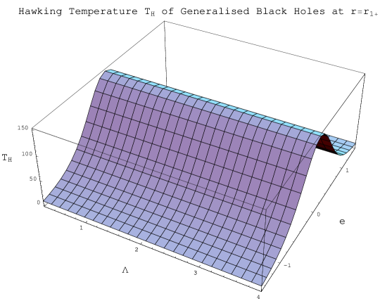
Figure 1: Hawking temperature $T_{H}$ at $r_{1+}$ versus cosmological constant $\Lambda$ and electric charge $e$

When $l=0,~{}k=1$ and $\Lambda=0$ in Eq.(30), the Hawking temperature of the accelerating and rotating BHs, electric and magnetic charges is recovered [8]. For $\alpha=0$, it reduces to the temperature of non-accelerating BHs [9], while $l=0,~{}k=1,~{}\alpha=0$, gives Hawking temperature of the Kerr-Newman BH [5], which further reduces to the temperature of the RN BH (for $a=0$). Finally, in the absence of charge, it exactly becomes the Hawking temperature of the Schwarzschild BH [24]. In case of massive particles ($m\neq 0$), following the same steps, we can obtain the same temperature. Thus the behavior will be same for both massive and massless particles near the BH horizon. For $\omega=1.25,M=10,\alpha=10,g=1,a=22,l=100$ (based on the cosmological constant $\Lambda$ and electric charge $e$), the graphical representation of Hawking temperature (30) (at $r=r_{1+}$) and the corresponding horizon $r=r_{1+}$ (3) of PD BHs is shown in Figures 1 and 2, respectively.

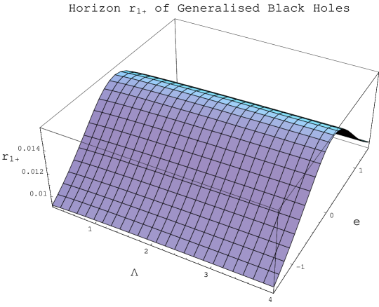
Figure 2: Horizon radius $r_{1+}$ versus cosmological constant $\Lambda$ and electric charge $e$

Now, we explore the tunneling probability of charged massive and massless fermions from the horizon $r_{2+}$ given in Eq.(4) by using the similar process. The corresponding set of Eqs.(LABEL:3)-(21) for the outgoing and incoming fermions, respectively, yield

$$R_{+}(r)=-R_{-}(r)=\left[\frac{\pi\iota[r_{2+}^{2}+(a+l)^{2}]\left(E-\Omega_{\alpha}J-\frac{qer_{2+}}{[r_{2+}^{2}+(a+l)^{2}]}\right)}{\left(r_{2+}-r_{1+}\right)\left(r_{2+}-r_{1-}\right)\left(r_{2+}-r_{2-}\right)}\right].$$ (31)

The probability for particles which tunnel through horizon will be

$$\Gamma = \exp\left[\frac{-4\pi[r_{2+}^{2}+(a+l)^{2}]\left(E-\Omega_{H}J-\frac{qer_{2+}}{[r_{2+}^{2}+(a+l)^{2}]}\right)}{\left(r_{2+}-r_{2-}\right)\left(r_{2+}-r_{1+}\right)\left(r_{2+}-r_{1-}\right)}\right].$$ (32)

Consequently, the corresponding temperature value (at $r_{2+}$) is

$$T_{H}=\left[\frac{\left(r_{2+}-r_{2-}\right)\left(r_{2+}-r_{1+}\right)\left(r_{2+}-r_{1-}\right)}{4\pi[r_{2+}^{2}+(a+l)^{2}]}\right].$$ (33)

For $\omega=9,~{}M=0.9,~{}\alpha=0.1,~{}g=15,~{}a=100,~{}l=10$, Figures 3 and 4 show that the Hawking temperature (33) at horizon radius $r_{2+}$ (4) always remains positive for the above mentioned parameters. The horizon radius $r_{2+}$ and Hawking temperature $T_{H}$ vanish as $\Lambda$ decreases and approach to zero for all $e$.

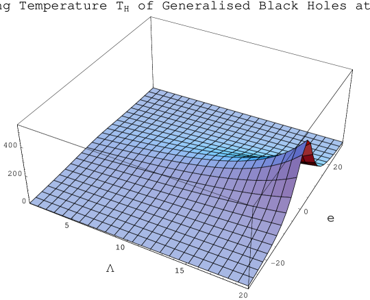
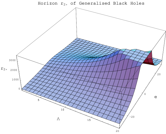
Figure 3: Hawking temperature $T_{H}$ at $r_{2+}$ versus cosmological constant $\Lambda$ and electric charge $e$

Figure 4: Horizon radius $r_{2+}$ versus cosmological constant $\Lambda$ and electric charge $e$

In general, both horizon temperatures will differ, but there is a set of parameters for which both temperatures have similar behavior at $r_{1+}$ and $r_{2+}$ given in Figures 5 and 6, respectively. The required set of parameters is given by $\omega=25,~{}M=50,~{}\alpha=12.5,~{}g=.01,~{}a=20,~{}l=100$.

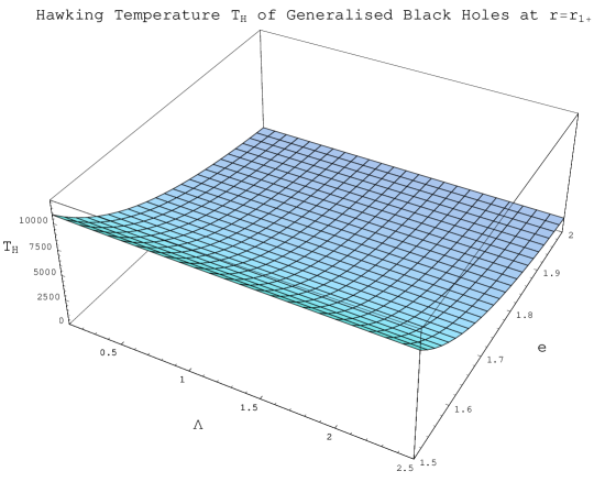
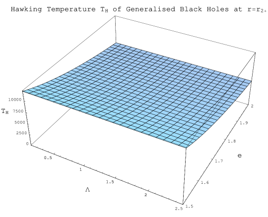
Figure 5: Hawking temperature $T_{H}$ at $r_{1+}$ versus cosmological constant $\Lambda$ and electric charge $e$

Figure 6: Hawking temperature $T_{H}$ at $r_{2+}$ versus cosmological constant $\Lambda$ and electric charge $e$

3.1 Action for the Emitted Particles

We evaluate particle’s action $I_{\uparrow}$ by using Eqs.(LABEL:3)-(21). For outgoing particles, Eqs.(LABEL:3) and (22) can be expressed as follows

$$R^{\prime}(r)=\frac{mA}{B\sqrt{(r-r_{+})\partial_{r}g(r_{+},\theta)}}-\frac{-E+\Omega_{H}J+\frac{qer_{+}}{[r_{+}^{2}+(a+l)^{2}]}}{(r-r_{+})\sqrt{\partial_{r}F(r_{+},\theta)\partial_{r}g(r_{+},\theta)}}.$$ (34)

Integration with respect to $r$ provides

$$R(r)=R_{+}(r)=\int\frac{mA}{B\sqrt{(r-r_{+})\partial_{r}g(r_{+},\theta)}}\textmd{d}r$$

$$-\frac{\left(-E+\Omega_{H}J+\frac{qer_{+}}{[r_{+}^{2}+(a+l)^{2}]}\right)}{\sqrt{\partial_{r}F(r_{+},\theta)\partial_{r}g(r_{+},\theta)}}\ln(r-r_{+}).$$ (35)

Similarly, in case of incoming particles, Eq.(LABEL:5) yields

$$R(r)=R_{-}(r)=\int\frac{mB}{A\sqrt{(r-r_{+})\partial_{r}g(r_{+},\theta)}}\textmd{d}r$$

$$+\frac{\left(-E+\Omega_{H}J+\frac{qer_{+}}{[r_{+}^{2}+(a+l)^{2}]}\right)}{\sqrt{\partial_{r}F(r_{+},\theta)\partial_{r}g(r_{+},\theta)}}\ln(r-r_{+}).$$ (36)

Using Eq.(22), we can write from Eqs.(19) or (21) as

$$\sqrt{\frac{P\Omega^{2}(r_{+},\theta)}{\rho^{2}(r_{+},\theta)}}\partial_{\theta}\Theta+\frac{\iota\rho(r_{+},\theta)\Omega(r_{+},\theta)}{\sqrt{\sin^{2}\theta P[r_{+}^{2}+(a+l)^{2}]^{2}}}$$ (37)

$$\times \left[J-q\left\{\frac{er_{+}[(l+a)^{2}-(l^{2}+a^{2}\cos^{2}\theta+2la\cos\theta)]}{a[r_{+}^{2}+(l+a\cos\theta)^{2}]}\right.\right.$$

$$+ \left.\left.\frac{g(l+a\cos\theta)[r_{+}^{2}+(l+a)^{2}]}{a[r_{+}^{2}+(l+a\cos\theta)^{2}]}\right\}\right]=0.$$

Inserting $\rho$ and $P$, after some manipulation, it follows that

$$\partial_{\theta}\Theta = \frac{\iota a\sin\theta[aJ+qer_{+}]}{[r_{+}^{2}+(a+l)^{2}]}\left[1-2\cos\theta\left\{\alpha\frac{a}{\omega}M\right.\right.$$

$$- \left.2\alpha^{2}l\frac{a}{\omega^{2}}(\omega^{2}k+e^{2}+g^{2})-\frac{2\Lambda}{3}al\right\}$$

$$- \left.\cos^{2}\theta\left\{-\alpha^{2}\frac{a^{2}}{\omega^{2}}(\omega^{2}k+e^{2}+g^{2})-\frac{\Lambda}{3}a^{2}\right\}\right]^{-1}$$

$$+ \frac{-\iota aJ+\iota qg(l+a\cos\theta)}{a\sin\theta}\left[1-2\cos\theta\left\{\alpha\frac{a}{\omega}M\right.\right.$$

$$- \left.2\alpha^{2}l\frac{a}{\omega^{2}}(\omega^{2}k+e^{2}+g^{2})-\frac{2\Lambda}{3}al\right\}$$

$$- \left.\cos^{2}\theta\left\{-\alpha^{2}\frac{a^{2}}{\omega^{2}}(\omega^{2}k+e^{2}+g^{2})-\frac{\Lambda}{3}a^{2}\right\}\right]^{-1}$$

$$+ \frac{\iota 2l(1-\cos\theta)[aJ+qer_{+}]}{\sin\theta[r_{+}^{2}+(a+l)^{2}]}\left[1-2\cos\theta\left\{\alpha\frac{a}{\omega}M\right.\right.$$

$$- \left.2\alpha^{2}l\frac{a}{\omega^{2}}(\omega^{2}k+e^{2}+g^{2})-\frac{2\Lambda}{3}al\right\}$$

$$- \left.\cos^{2}\theta\left\{-\alpha^{2}\frac{a^{2}}{\omega^{2}}(\omega^{2}k+e^{2}+g^{2})-\frac{\Lambda}{3}a^{2}\right\}\right]^{-1}.$$

Integrating with respect to $\theta$, we have

$$\Theta=\frac{\iota a[aJ+qer_{+}]}{[r_{+}^{2}+(a+l)^{2}]}I_{1}+I_{2}+\frac{2l\iota[aJ+qer_{+}]}{[r_{+}^{2}+(a+l)^{2}]}I_{3},$$ (38)

where $I_{1},~{}I_{2}$ and $I_{3}$ are given as follows

$$I_{1} = \int\left[\frac{\sin\theta}{1-2\tilde{A}\cos\theta-\tilde{B}\cos^{2}\theta}\right]\textmd{d}\theta,$$

$$I_{2} = \int\left[\frac{\iota qg(l+a\cos\theta)-\iota aJ}{a\sin\theta[1-2\tilde{A}\cos\theta-\tilde{B}\cos^{2}\theta]}\right]\textmd{d}\theta,$$

$$I_{3} = \int\left[\frac{1-\cos\theta}{\sin\theta[1-2\tilde{A}\cos\theta-\tilde{B}\cos^{2}\theta]}\right]\textmd{d}\theta,$$

and

$$\tilde{A} = \left[\alpha\frac{a}{\omega}M-2\alpha^{2}l\frac{a}{\omega^{2}}(\omega^{2}k+e^{2}+g^{2})-\frac{2\Lambda}{3}al\right],$$

$$\tilde{B} = \left[-\alpha^{2}\frac{a^{2}}{\omega^{2}}(\omega^{2}k+e^{2}+g^{2})-\frac{\Lambda}{3}a^{2}\right].$$

Solving these integrals, we obtain after some algebra

$$I_{1} = \left[\frac{1}{2\sqrt{\tilde{A}^{2}+\tilde{B}}}\ln\left[\frac{1-x(\tilde{A}+\sqrt{\tilde{A}^{2}+\tilde{B}})}{1-x(\tilde{A}-\sqrt{\tilde{A}^{2}+\tilde{B}})}\right]\right],$$ (39)

$$I_{2} = L_{1}\ln\left[\frac{1-x(\tilde{A}+\sqrt{\tilde{A}^{2}+\tilde{B}})}{1-x(\tilde{A}-\sqrt{\tilde{A}^{2}+\tilde{B}})}\right]+L_{2}\ln\left[1-2\tilde{A}x-\tilde{B}x^{2}\right]$$ (40)

$$+ L_{3}\ln[1-\cos\theta]+L_{4}\ln[1+\cos\theta],$$

where

$$L_{1} = \left[\frac{1}{2\sqrt{\tilde{A}^{2}+\tilde{B}}[(1-\tilde{B})^{2}-4\tilde{A}^{2}]}\right]\left[\iota J(2\tilde{A}^{2}-\tilde{B}^{2}+\tilde{B})\right.$$

$$+ \left.\iota qg(-\tilde{A}+\frac{l}{a}\tilde{B}^{2}-2\frac{l}{a}\tilde{A}^{2}-\frac{l}{a}\tilde{B}-\tilde{A}\tilde{B})\right],$$

$$L_{2} = \frac{1}{[(1-\tilde{B})^{2}-4\tilde{A}^{2}]}\left[\iota J\tilde{A}-\frac{\iota qg}{2}(1-\tilde{B}+2\frac{l}{a}\tilde{A})\right],$$

$$L_{3} = \frac{1}{2(1-2\tilde{A}-\tilde{B})}\left[\iota qg(\frac{l}{a}+1)-\iota J\right],$$

$$L_{4} = \frac{1}{2(1-\tilde{B}+2\tilde{A})}\left[\iota J+\iota qg(-\frac{l}{a}+1)\right]$$

and $I_{3}$ can be obtained as

$$I_{3} = N_{1}\ln\left[\frac{1-x(\tilde{A}+\sqrt{\tilde{A}^{2}+\tilde{B}})}{1-x(\tilde{A}-\sqrt{\tilde{A}^{2}+\tilde{B}})}\right]$$ (41)

$$+ N_{2}\ln\left[1-2\tilde{A}x-\tilde{B}x^{2}\right]+N_{3}\ln[1+x],$$

where $x=\cos\theta$ and

$$N_{1} = \left[\frac{\tilde{A}-\tilde{B}}{2\sqrt{\tilde{A}^{2}+\tilde{B}}(1-\tilde{B}+2\tilde{A})}\right],$$

$$N_{2} = \left[\frac{1}{2(1-\tilde{B}+2\tilde{A})}\right],\quad N_{3}=-\left[\frac{1}{(1-\tilde{B}+2\tilde{A})}\right].$$

Equations (22), (35) and (38) can determine the value for $W(r,\theta)$ and hence the outgoing massive particles action can be obtained. For $m=0$, this expression diminishes to the massless particles action. Similarly, we can determine the action for the incoming particles either massive or massless.

4 Outlook

In this paper, we have used semiclassical WKB approximation to study tunneling continuum of charged fermions from a pair of electrically and magnetically charged accelerating and rotating BHs, together with NUT parameter and cosmological constant. It is found that the tunneling probabilities ((28) and (32)) of outgoing charged fermions do not depend upon fermion’s mass but only its charge. For the family of BH solutions, the corresponding Hawking temperatures ((30) and (33)) depend upon mass, acceleration, rotation parameters and NUT parameter as well as electric and magnetic charges of the pair of BHs involving cosmological constant. Equations for the spin-down case are of the identical form as in case of the spin-up particles with the exception of negative sign. For both cases, either massive or massless, the Hawking temperature indicates that the spin-up and spin-down particles are transmitted at the similar tunneling rate [4].

This work is the generalization of our previous work [17] by adding $\Lambda$ in the family of BH solutions. We see from graphs that these solutions lead to expanding BH solutions. We would like to mention here that the cosmological constant can be positive/negative in general. However, for the sake of positive temperature, the cosmological constant must be positive for this set of parameters. We can take negative cosmological constant for some other set of parameters but it is not sure whether it will give temperature positive or negative. It is worth mentioning here that for the PD family of BH solutions, in the absence of the cosmological constant, all results reduce to the results already given in [17].

The graphical representation (Figures 1 and 2) indicates that whether the cosmological constant increases or decreases, it has no effect on the horizon radius $r_{1+}$. However, the horizon radius always increases (hence approaches to its maximum value) whether $e$ is decreasing to zero or increasing to zero. Similarly, the horizon radius always decreases (hence approaches to its minimum value) whether positive $e$ is increasing to $+\infty$ or negative $e$ is decreasing to $-\infty$. Hawking temperature remains positive for this choice of parameters. For $e<0$, the temperature decreases as $e$ decreases (independent of $\Lambda$). For $e>0$, the temperature increases as $e$ decreases. For $e=0$, temperature approaches to its maximum value, while $\Lambda$ behaves constantly. We see from Figures 3 and 4 that for increasing $\Lambda$, the temperature $T_{H}$ and radius $r_{2+}$ increase when $e<0$, while these decrease when $e>0$. For $e=0$, the Hawking temperature and horizon radius attain its maximum values with positive increasing $\Lambda$.

The graphical behavior of horizons show that $r_{1+}$ is the outer horizon, while $r_{2+}$ is the cosmological horizon. In the tunneling picture, particles can also tunnel from the cosmological horizon like the event horizon. The tunneling behavior is different for these two horizons. The event horizon decreases when +ve-energy particles tunnel across it, while the cosmological horizon expands. The emitted particles are found to tunnel into the cosmological horizon in the form of radiation [24]-[26].

For de Sitter BHs, particles can be created at event horizon as well as at cosmological horizon. At the event horizon, $+$ve-energy (outgoing) particles tunnel out the BH horizon to form Hawking radiation and $-$ve-energy (incoming) particles can fall into the horizon along classically permitted trajectories. At the cosmological horizon, outgoing particles can fall classically out of the horizon and incoming particles tunnel inside the horizon to form Hawking radiation for distant observer. Thus, the tunneling probability of incoming particles through cosmological horizon $r_{2+}$ of PD BHs can be written as

$$\Gamma = \frac{\textmd{Prob}[\textmd{in}]}{\textmd{Prob}[\textmd{out}]}=\exp[-4\textmd{Im}R_{-}],$$

$$= \exp\left[\frac{4\pi\left[r_{2+}^{2}+(a+l)^{2}\right]\left(E-\Omega_{H}J-\frac{qer_{2+}}{\left[r_{2+}^{2}+(a+l)^{2}\right]}\right)}{\left(r_{2+}-r_{1+}\right)\left(r_{2+}-r_{1-}\right)\left(r_{2+}-r_{2-}\right)}\right].$$

By comparing the above expression with the Boltzmann factor, there is only one choice to consider $-$ve-energy at cosmological horizon. Thus, in de Sitter space massive particles have $-$ve-energy which can tunnel inside the cosmological horizon. The Hawking temperature at the cosmological horizon of PD BHs by using $-$ve-energy particles can be written as given by Eq.(33). This temperature is same as for the temperature of outgoing particles.

Figures 1 and 3 show that the Hawking temperatures at horizon radii $r_{1+}$ and $r_{2+}$ exhibit $+$ve behavior. Thus the Hawking temperatures (30) and (33) must be $+$ve for outgoing particles through the event horizon and incoming particles through the cosmological horizon. The graphical behavior of temperature helps to know about the horizon radii of PD BH. These verifications are consistent with already available in the literature [7].

Finally, it is pointed out that BHs with NUT charge are not consistent with the existence of fermions insofar as such spacetimes do not support spin structures [27]. Here we have given calculations that surprisingly show good agreement with known results about the Hawking temperature in the limits in which they apply. This agreement is of particular interest even when no spin structure of $\Psi$ exists.

Acknowledgement

We would like to thank the Higher Education Commission, Islamabad, Pakistan, for its financial support through the Indigenous Ph.D. 5000 Fellowship Program Batch-IV. We also appreciate the referee’s comments and providing a particular reference.