Classical simulation of quantum dephasing and depolarizing noise

Abstract

Dephasing decoherence induced by interaction of one qubit with a quantum bath can be simulated classically by random unitary evolution without the need for a bath and this random unitary evolution is equivalent to the quantum case.  For a general dephasing model and a single qubit system, we explicitly construct the noise functional and completely specify the random unitary evolution.  To demonstrate the technique, we applied our results to three paradigmatic models: spin-boson, central spin, and quantum impurity.  For multiple qubits, we identify a class of generalized quantum dephasing models that can be simulated classically. Finally we show that depolarizing quantum models can be simulated classically for all dimensionalities of the principal system.

I Introduction

The notion of an open quantum system has received intense scrutiny in recent years, motivated initially by questions about the location and nature of the boundary (if any) between the quantum and classical worlds Caldeira and Leggett (1983). Further impetus has been given by the desire to minimize decoherence in quantum information processing Nielsen and Chuang (2000); Weiss (1999).  Open quantum systems have been conceived in two quite distinct ways: a system and bath considered as a single quantum entity with overall unitary dynamics, or a quantum system acted on by random classical forces.  The first (system-bath or SB) approach is usually thought of as being more general since it includes the transformation of information and the idea that decoherence is connected to the entanglement of a system with its environment Palma et al. (1996).  In the random classical (RC) force approach these effects are absent.  Furthermore, in the question of the quantum-classical divide, it is often seen as important that the bath be macroscopic since this precludes the complete measurement of the bath degrees of freedom.

It is very clear from the Kraus operator representation that the SB approach is more general than the RC one, since the operators need not be unitary in SB.  However, this does not illuminate what precisely is the role of entanglement in separating the SB and RC methods.  In fact, it has been pointed out that SB models whose coupling is of dephasing type should always be able to be rewritten as classical models Helm et al. (2011).  This is based on general results concerning existence of certain positive maps Landau and Streater (1993).  A specific example of a single qubit bath has been given Helm and Strunz (2009).  Since SB entanglement is present in many dephasing models, this implies that this entanglement is not the decisive feature of SB models that distinguishes them from RC models.

In order to understand this particular aspect of the difference between quantum theory and classical physics, we seek to find situations in which SB models can be classically simulated.  There are two aspects to this program.  The first is existence: which SB models can be classically simulated?  The second is construction: can we write down explicitly the RC model that corresponds to a given SB model?  The possibility of such simulation of course does not imply that system-bath entanglement is not important for quantum decoherence, but it does imply that the distinction between quantum and classical noise is more subtle than has been previously recognized.

The existence question for one qubit has been essentially settled in Refs. Helm et al. (2011) and Helm and Strunz (2009). We extend this work by giving an explicit construction method.  As examples, we show explicitly how three paradigmatic system-macroscopic dephasing bath models can be simulated by subjecting the quantum 2-level system to a classical random force without ever needing the bath.  We do this by describing completely the classical noise source that perfectly mimics the effect of entanglement of the qubit with the bath (Sec. II).   The three models are the popular spin-boson model, a specific central spin model, and the quantum impurity model (Sec. III).  The last model is particularly interesting in this context since it has a “classical” and a “quantum” phase Grishin et al. (2005). For multiple qubits, we can also give a construction method for a certain class of multiple-qubit dephasing models, extending both existence and construction results.   The qubits can be interacting and entangled, so the generalization is non-trivial (Sec. IV).  Finally we show that pure depolarizing models on qudits of arbitrary dimension can always be simulated classically (Sec. V).

II Classical Simulation of Quantum Dephasing Models

II.1 Quantum Models

The class of quantum models considered in this section consists of a single qubit principal system subject to dephasing by an arbitrary quantum system.  Thus the total Hamiltonian of the composite system is

$$H=H_{S}\left[\sigma_{i}\right]+H_{B}\left[\lambda_{i}\right]+H_{SB}\left[\sigma_{i},\lambda_{i}\right]$$ (1)

where $\sigma_{0,x,y,z}$ are the identity matrix $I$ and the Pauli matrices that act on the qubit and the matrices $\lambda_{j}$ are some complete set of Hermitian operators for the bath, taken for simplicity to be finite-dimensional.  $H_{B}\left[\lambda_{i}\right]+H_{SB}\left[\sigma_{i},\lambda_{i}\right]$ are linear functions of the $\lambda_{i}.$  $\lambda_{0}$ is proportional to the identity, and $\operatorname{Tr}_{B}$ $\lambda_{i}=0$ for $i>0.$  For an $N$-level bath the $\lambda_{i}$ for $i>0$ could be chosen as proportional to the $N^{2}-1$ generators of $SU\left(N\right)$ and $\lambda_{0}=I/N.$  $\operatorname{Tr}_{B}$ is the trace over bath variables.  We shall normalize the $\lambda_{i}$ by the condition that $\operatorname{Tr}_{B}\left[\lambda_{i}\lambda_{j}\right]=\delta_{ij}$ for $i,j>0.$  $H_{B}\left[\lambda_{i}\right]$ is the bath Hamiltonian.  Infinite-dimensional baths can be treated by the same method at the cost of some additional notational complexity.

We will focus on dephasing models, defined as those for which $\left[H_{S},H_{SB}\right]=0.$

The total density matrix can be expanded as

$$\rho=\sum_{ij}N_{ij}\sigma_{i}\otimes\lambda_{j}$$ (2)

and we can invert this equation :

$$N_{ij}=\frac{1}{2}\operatorname{Tr}\left[\left(\sigma_{i}\otimes\lambda_{j}\right)\rho\right].$$

The reduced density matrix of the system is

$$\rho^{S}=\operatorname{Tr}_{B}\rho=\frac{1}{2}\sum_{i}n_{i}\sigma_{i}$$

and $n_{i}=\left(1,n_{x},n_{y},n_{z}\right)$ is the expanded Bloch vector of the system. For quantum noise we have

$$\rho\left(t\right)=U\rho\left(0\right)U^{{\dagger}}$$

with $U=\exp\left(-iHt\right)$ where we have set $\hbar=1$.  In terms of components this is

$$N_{ij}\left(t\right)=\frac{1}{2}\sum_{kl}\operatorname{Tr}\left[\left(\sigma_{i}\otimes\lambda_{j}\right)U\left(\sigma_{k}\otimes\lambda_{l}\right)U^{{\dagger}}\right]N_{kl}\left(0\right).$$

We assume that the initial $\rho$ is in a product form $\rho\left(0\right)=\rho^{S}\left(0\right)\otimes\rho^{B}\left(0\right),$ which in components says that $N_{ij}\left(0\right)=\frac{1}{2}n_{i}\left(0\right)m_{j},$ where

$$m_{j}=\operatorname{Tr}_{B}\lambda_{i}\rho^{B}\left(0\right).$$

This is an important assumption, which will be used throughout the rest of the paper.  It is an open question whether the results below can be generalized to non-product initial conditions.  The dynamics of the system can be rewritten as

$$N_{ij}\left(t\right)=\frac{1}{2}\sum_{kl}\operatorname{Tr}\left[\left(\sigma_{i}\otimes\lambda_{j}\right)U\left(\sigma_{k}\otimes\lambda_{l}\left(0\right)\right)U^{{\dagger}}\right]n_{k}\left(0\right)m_{l}$$

and the Bloch vector of the qubit at time $t$ is given by

$$n_{i}\left(t\right) =2N_{i0}\left(t\right)$$

$$=\sum_{kl}\operatorname{Tr}\left[\left(\sigma_{i}\otimes\lambda_{0}\right)U\left(\sigma_{k}\otimes\lambda_{l}\right)U^{{\dagger}}\right]n_{k}\left(0\right)m_{l}$$

Finally we have a linear relation between the initial and final expanded Bloch vectors:

$$n_{i}\left(t\right)=\sum_{k}T_{ik}^{\left(Q\right)}n_{k}\left(0\right)$$

where the quantum transfer matrix is given by

$$T_{ik}^{\left(Q\right)}\left(t\right)=\sum_{l}\operatorname{Tr}\left[\left(\sigma_{i}\otimes\lambda_{0}\right)U\left(\sigma_{k}\otimes\lambda_{l}\right)U^{{\dagger}}\right]m_{l}.$$ (3)

One should note that this represents a linear relation between the initial and final expanded Bloch vectors.  However, if construed as a relation between the usual 3-dimensional Bloch vectors, it is an affine relation, since if $n_{i}\left(t=0\right)=\left(1,0,0,0\right),$ then the initial state has zero ordinary Bloch vector, but the final state has $n_{i}\left(t\right)=T_{i0}^{\left(Q\right)},$ which is not zero.  Expanding the Bloch vector to four components is just a convenient way of including the affine part.

The whole dynamics of the qubit is contained in the matrix $T_{ik}^{\left(Q\right)}\left(t\right).$  Given a Hamiltonian for the coupled system and bath, $V$, the matrix $T_{ik}^{\left(Q\right)}\left(t\right)$ is uniquely defined by Eq. 3.  More formally, let us define the set $QM$ of quantum models specified by $H$ and $U.$  Let $qm\in QM$ be a member of this set.  Let $RS$ be the set of all evolutions of the density matrix of the principal system and let $rs\in RS$ be a member of this set.  Then Eq. 3 defines a map $f:QM\rightarrow RS.$

II.2 Classical Noise

A 2-level system acted on by dephasing classical noise has the $2\times 2$ Hamiltonian

$$H_{Cl}=-\frac{1}{2}B\sigma_{z}+\frac{1}{2}h\left(t\right)\sigma_{z}.$$ (4)

$h\left(t\right)$ is a random classical (c-number) function of time that represents an external source of noise.  To completely specify the model we need a probability functional $\mathcal{P}\left[h\right]$ on the noise histories.  Then the system dynamics is given by

$$\rho^{\left(Cl\right)}\left(t\right)= \int\mathcal{D}\left[h\left(t^{\prime}\right)\right]\mathcal{P}\left[h\left(t^{\prime}\right)\right]$$ (5)

$$\times U_{Cl}\left[h\left(t^{\prime}\right)\right]\rho^{\left(Cl\right)}\left(0\right)U_{Cl}^{{\dagger}}\left[h\left(t^{\prime}\right)\right].$$

This is a functional integral over all real functions $h\left(t^{\prime}\right)$ defined on the interval $0\leq t^{\prime}\leq t.$  Each $h\left(t^{\prime}\right)$ is assigned a probability $\mathcal{P}\left[h\left(t^{\prime}\right)\right]$ and

$$\int\mathcal{D}\left[h\left(t^{\prime}\right)\right]\mathcal{P}\left[h\left(t^{\prime}\right)\right]=1.$$

Here the time-ordered exponential $U_{Cl}\left[h\left(t\right)\right]=\mathcal{T}\exp\left(-i\int_{0}^{t}H_{Cl}\left(t^{\prime}\right)~{}dt^{\prime}\right)$ is a $2\times 2$ matrix, unlike $U_{Q}\left(t\right),$ which is infinite-dimensional. In the dephasing case two Hamiltonians taken at different times commute: $\left[H_{Cl}\left(t\right),H_{Cl}\left(t^{\prime}\right)\right]=0$ and the time-ordering can be dropped.  Note the simplicity of the classical problem relative to the quantum one.

We now follow the steps of the discussion of the quantum models with the appropriate modifications. Restating the results in terms of the $3\times 3$ transfer matrix $T^{\left(Cl\right)},$ we have, in exact analogy to the section  above,

$$\rho^{S} =\frac{1}{2}\sum_{i=0}^{3}n_{i}\sigma_{i},$$

$$n_{i} =\frac{1}{2}\operatorname{Tr}\sigma_{i}\rho^{S}$$

$$n_{i}\left(t\right) =\sum_{j=0}^{3}T_{ij}^{\left(Cl\right)}\left(t\right)n_{j}\left(0\right)$$

where

$$T_{ij}^{\left(Cl\right)}\left(t\right)= \frac{1}{2}\int\mathcal{D}\left[h\left(t^{\prime}\right)\right]\mathcal{P}\left[h\left(t^{\prime}\right)\right]\times$$ (6)

$$\operatorname{Tr}\left\{\sigma_{i}U_{Cl}[h\left(t^{\prime}\right)]\sigma_{j}U_{Cl}^{{\dagger}}[h\left(t^{\prime}\right)]\right\}$$

Note that $T_{i0}^{\left(Cl\right)}=\frac{1}{2}\operatorname{Tr}\sigma_{i}=\delta_{i0},$ so the classical model always gives a linear relation between initial and final ordinary Bloch vectors— there is no affine term.  This is another example of the fact that not all quantum models have a classical analog.  A simple example of an affine evolution is a qubit initially in equilibrium at high temperature that is cooled by a bath.  Then we have that $\rho^{S}\left(t=0\right)\approx I/2,$ whereas at long times the system will be at thermal equilibrium at a lower temperature and the state populations will be determined by the Boltzmann factor.  This physical process cannot be mimicked by classical external noise in the sense of random unitary evolution.

Define the set $CM$ of quantum models specified by $H_{cl}$ and $\mathcal{P}.$  Then Eq.  6 defines a map $g:CM\rightarrow RS$.

II.3 Classical Simulation of Quantum Models

To demonstrate the quantum-classical equivalence we need to prove the existence of a functional $\mathcal{P}\left[h\left(t\right)\right]$ such that $\rho_{S}^{\left(Cl\right)}\left(t\right)=\rho_{S}^{\left(Q\right)}\left(t\right),$ or, equivalently that $T_{ik}^{\left(Cl\right)}\left(t\right)=T_{ik}^{\left(Q\right)}\left(t\right).$ For dephasing models we shall do more than this— we shall give the explicit construction of the classical model.

In the construction we shall need only the discrete version of Eq. (5), which is

$$\rho^{\left(Cl\right)}\left(t\right)=\sum_{r}p_{r}U_{Cl}^{\left(r\right)}\rho^{\left(Cl\right)}\left(t=0\right)U_{Cl}^{\left(r\right){\dagger}},$$

where $r$ labels the possible noise histories and $U_{Cl}^{\left(r\right)}$ is the evolution operator for that history. The positive numbers $p_{r}$ satisfy  $\sum_{r}p_{r}=1.$  The corresponding statement for the Bloch vector is

$$n_{i}\left(t\right)=\sum_{k,r}p_{r}O_{ik}^{\left(r\right)}\left(t\right)n_{k}\left(0\right),$$ (7)

and the $O_{ik}^{\left(r\right)}$ are orthogonal matrices for every $r.$  Thus the problem of showing that a quantum noise model is actually classical reduces to the problem of showing that the matrix $T_{ik}^{\left(Q\right)}$ can be written as a convex combination of orthogonal matrices.

We shall consider the system-bath model for one qubit of Eq. (1).  Without loss of generality we choose the total Hamiltonian

$$H=-\frac{1}{2}B\sigma_{z}+H_{B}\left[\lambda_{i}\right]+H_{SB}\left[\lambda_{i}\right]\sigma_{z};$$ (8)

so that the qubit has no non-trivial dynamics and the noise is pure dephasing.

In this model $\sigma_{z}$ is conserved, which implies that

$$T_{zz}^{\left(Q\right)}=1\;;\;T_{xz}^{\left(Q\right)}=T_{zx}^{\left(Q\right)}=T_{yz}^{\left(Q\right)}=T_{zy}^{\left(Q\right)}=0\text{.}$$

We also have that $T_{00}^{\left(Q\right)}=1$ and $T_{i0}^{\left(Q\right)}=T_{0i}^{\left(Q\right)}=0$ for $i>0,$ so we only need to calculate $T_{xx}^{\left(Q\right)},T_{yy}^{\left(Q\right)},T_{xy}^{\left(Q\right)}$ and $T_{yx}^{\left(Q\right)}.$

First we note that the total evolution operator is

$$U_{Q}=\mathcal{T}\exp\left(-i\int_{0}^{t}H\left(t^{\prime}\right)dt^{\prime}\right)=u\left(t\right)+v\left(t\right)~{}\sigma_{z},$$ (9)

where $u\left(t\right)$ and $v\left(t\right)$ are time-dependent bath operators and $\mathcal{T}$ denotes time-ordering.  Explicitly,

$$u\left(t\right) =\frac{1}{2}\operatorname{Tr}_{S}\left[\mathcal{T}\exp\left(-i\int_{0}^{t}H\left(t^{\prime}\right)dt^{\prime}\right)\right]$$ (10)

$$v\left(t\right) =\frac{1}{2}\operatorname{Tr}_{S}\left[\sigma_{z}\mathcal{T}\exp\left(-i\int_{0}^{t}H\left(t^{\prime}\right)dt^{\prime}\right)\right],$$

where $\operatorname{Tr}_{S}$ is the trace over qubit variables.  In Eq. 9 the time ordering is essential, since the $\lambda_{i}$ do not commute with one another.  Note that these expressions do not depend in any way on having a finite-dimensional bath.  Since $I=UU^{{\dagger}}$ we have

$$uu^{{\dagger}}+vv^{{\dagger}} =I$$

$$uv^{{\dagger}}+vu^{{\dagger}} =0.$$

Expressing $T^{\left(Q\right)}$ in terms of $u$ and $v$ we find

$$T_{xx}^{\left(Q\right)}\left(t\right) =T_{yy}^{\left(Q\right)}\left(t\right)$$ (11)

$$=\operatorname{Tr}\left[\left(u^{{\dagger}}+v^{{\dagger}}\sigma_{z}\right)\left(\sigma_{x}\otimes\lambda_{0}\right)\left(u+v\sigma_{z}\right)\left(\sigma_{x}\otimes\rho^{B}\left(0\right)\right)\right]$$

$$=2\operatorname{Tr}_{B}\left[\left(u^{{\dagger}}u-v^{{\dagger}}v\right)\rho^{B}\left(0\right)\right]$$

$$T_{xy}^{\left(Q\right)}\left(t\right) =-T_{yx}^{\left(Q\right)}\left(t\right)$$ (12)

$$=\operatorname{Tr}_{B}\left[\left(u^{{\dagger}}+v^{{\dagger}}\sigma_{z}\right)\left(\sigma_{x}\otimes\lambda_{0}\right)\left(u+v\sigma_{z}\right)\left(\sigma_{y}\otimes\rho^{B}\left(0\right)\right)\right]$$

$$=\operatorname{Tr}_{B}\left[\left(-2iu^{{\dagger}}v+2iv^{{\dagger}}u\right)\rho^{B}\left(0\right)\right],$$

and defining $c=T_{xx}^{\left(Q\right)}=T_{yy}^{\left(Q\right)}$ and $s=-T_{xy}^{\left(Q\right)}=T_{yx}^{\left(Q\right)}$, the matrix $T^{\left(Q\right)}$ has the form

$$T^{\left(Q\right)}=\begin{pmatrix}1&0&0&0\\ 0&c&-s&0\\ 0&s&c&0\\ 0&0&0&1\end{pmatrix}.$$

with positivity implying that $c^{2}+s^{2}=r^{2}\leq 1.$  The submatrix $T_{ij}^{\left(Q\right)}$ with $i,j=x,y$ is proportional to an orthogonal $2\times 2$ matrix.  All effects of the bath on the system are summarized by the quantities $c\left(t\right)$ and $s\left(t\right).$

The task is now to construct the equivalent classical model.  In two dimensions, an orthogonal matrix $M$ is characterized by a single unit vector $\left(\cos\theta,\sin\theta\right),$ so a convex sum of orthogonal matrices is of the form

$$\sum\limits_{i}p_{i}M_{i}=\begin{pmatrix}\sum\limits_{i}p_{i}\cos\theta_{i}&-\sum\limits_{i}p_{i}\sin\theta_{i}\\ \sum\limits_{i}p_{i}\sin\theta_{i}&\sum\limits_{i}p_{i}\cos\theta_{i}\end{pmatrix},$$

with $p_{i}>0$ and $\sum_{i}p_{i}=1.$  This matrix is proportional to the $i,j=x,y$ submatrix of $T_{ij}^{\left(Q\right)}.$

We first write the vector $\left(c,s\right)$ as the convex sum of unit vectors:

$$\begin{pmatrix}c\\ s\end{pmatrix}=\frac{1}{2}\begin{pmatrix}c+\beta s\\ s-\beta c\end{pmatrix}+\frac{1}{2}\begin{pmatrix}c-\beta s\\ s+\beta c\end{pmatrix}$$

where

$$r^{2}=c^{2}+s^{2}=\left[T_{xx}^{\left(Q\right)}\right]^{2}+\left[T_{xy}^{\left(Q\right)}\right]^{2}\;;\;\beta=\frac{\sqrt{1-r^{2}}}{r}$$ (13)

This decomposition of the vector $\left(c,s\right)$ is not unique.  This implies that the mapping $g:CM\rightarrow RS$ is not injective.

Then the classical evolution submatrix is written as

$$T^{\left(Cl\right)}=\frac{1}{2}\begin{pmatrix}\cos\Phi_{1}&-\sin\Phi_{1}\\ \sin\Phi_{1}&\cos\Phi_{1}\end{pmatrix}+\frac{1}{2}\begin{pmatrix}\cos\Phi_{2}&-\sin\Phi_{2}\\ \sin\Phi_{2}&\cos\Phi_{2}\end{pmatrix}.$$

$T^{\left(Cl\right)}$ is the convex sum of rotations through the two angles

$$\Phi_{1}\left(t\right)= \tan^{-1}\left(\frac{s-\beta c}{c+\beta s}\right)$$ (14)

and

$$\Phi_{2}\left(t\right)= \tan^{-1}\left(\frac{s+\beta c}{c-\beta s}\right).$$

Hence, by comparison to Eq. (7), it defines a classical model.  Define the fields $h_{1}\left(t\right)$ and $h_{2}\left(t\right)$ by

$$h_{1}= \frac{\partial\Phi_{1}}{\partial t}+B$$ (15)

and

$$h_{2}= \frac{\partial\Phi_{2}}{\partial t}+B.$$

Then the equivalent classical model is given by

$$H_{Cl}=-\frac{1}{2}B\sigma_{z}+\frac{1}{2}h\left(t\right)\sigma_{z}$$

and the probability distribution for $h$ is: $h\left(t\right)=h_{1}\left(t\right)$ with probability $1/2$ and $h\left(t\right)=h_{2}\left(t\right)$ with probability $1/2.$   More formally, $\mathcal{P}\left[h\left(t\right)\right]=\left(1/2\right)\delta\left[h-h_{1}\right]+\left(1/2\right)\delta\left[h-h_{2}\right].$  Writing $\Phi_{i}\left(t\right)=\int_{0}^{t}\left(-B+h_{i}\left(t^{\prime}\right)\right)dt^{\prime}$ and following Eq. (6) we find

$$T_{ij}^{\left(Cl\right)}= \frac{1}{4}\operatorname{Tr}\left[\sigma_{i}e^{\frac{i}{2}\sigma_{z}\Phi_{1}\left(t\right)}\sigma_{j}e^{-\frac{i}{2}\sigma_{z}\Phi_{1}\left(t\right)}\right]$$

$$+\frac{1}{4}\operatorname{Tr}\left[\sigma_{i}e^{\frac{i}{2}\sigma_{z}\Phi_{2}\left(t\right)}\sigma_{j}e^{-\frac{i}{2}\sigma_{z}\Phi_{2}\left(t\right)}\right]$$

The contents of this section can be summarized by the following theorem and constructive proof.

Theorem.

The dynamics of the open quantum system given by Eq. (8) can be simulated by the classical noise model given by Eq. (4) with $h(t)$ given by Eqs. (15); the density matrix of the qubit is the same for the two models at all times.

Proof.

The quantum Hamiltonian $H$ of Eq. (8) determines the noise functions $u(t)$ and $v\left(t\right)$ in Eqs. (10) and hence the matrix $T^{\left(Q\right)}$ in Eqs. (11) and (12) uniquely.  The classical fields $h_{1}\left(t\right)$ and $h_{2}\left(t\right)$ are given explicitly in terms of the matrix elements of $T^{\left(Q\right)}$ by Eqs. (13) through (15).  $h_{1}\left(t\right)$ and $h_{2}\left(t\right)$ in turn define the classical Hamiltonian $H_{Cl}$ and noise probability functional $\mathcal{P}$ given in Eqs. (4) and (5).  The evolution of the qubit density matrix according to $H_{Q}$ with the usual partial trace is precisely the same as the qubit evolution according to the classical Hamiltonian $H_{Cl}$ with the averaging over noise histories. ∎

II.4 Equivalent Classical and Quantum Models

Our terminology is to call a classical model equivalent to a quantum one if $rs\in RS,$ the evolution of the principal system, is the same.  More precisely, we say that $qm$ is equivalent to $cm$ if there exists $rs$ such that $f\left(qm\right)=rs$ and $g\left(cm\right)=rs.$  We now complete our characterization of $f$ using a standard method Nielsen and Chuang (2000), that immediately implies that many quantum models correspond to any particular $rs$.  The proof is as follows.  It is not restricted to single qubits.  Let the principal system have an $S$-dimensional Hilbert space $\mathcal{H}_{S}.$  An RC model has an EPS of the form

$$\rho_{S}\left(t\right)=\sum_{\alpha}M_{\alpha}\left(t\right)\rho_{S}\left(0\right)M_{\alpha}^{{\dagger}}\left(t\right),$$ (16)

where $M_{\alpha}=\sqrt{p_{\alpha}}U_{\alpha},$ and $U_{\alpha}$ is the unitary operator corresponding to the $\alpha$-th history of the classical noise; $p_{\alpha}$ is the probability of that noise.  $\rho_{S}$ is an $S\times S$ matrix.  We then construct the equivalent quantum model as follows.  There is a bath, which is a $D$-dimensional quantum system with Hilbert space $\mathcal{H}_{B}$ which has basis states $\left\{\left|0\right\rangle_{B},\left|1\right\rangle_{B},\left|2\right\rangle_{B},...,\left|D-1\right\rangle_{B}\right\}.$  We associate a bath state $\left|\alpha\right\rangle_{B}$ with each of the classical histories $\alpha$. The bath is in the initial state $\left|0\right\rangle_{B}$ and the total initial state is:

$$\rho_{T}\left(t=0\right)=\rho_{S}\otimes\left|0\right\rangle_{B}~{}\left\langle 0\right|_{B}.$$ (17)

The assumption that the environment is in a pure state is not too restrictive since we can increase $D$ and purify the state if we wish.  The product form is restrictive, however, as already stated.  We now need a total evolution operator $U_{T}$ that is an $\left(SD\times SD\right)$ unitary matrix that acts on the coupled system and bath, i.e., it acts in the Hilbert space $\mathcal{H}_{B}\otimes\mathcal{H}_{S}.$  We partially define it by

$$U_{T}\left(\left|n\right\rangle_{S}\otimes\left|0\right\rangle_{B}\right)=\sum_{\alpha=0}^{D-1}M_{\alpha}~{}\left|n\right\rangle_{S}~{}\otimes\left|\alpha\right\rangle_{B}.$$ (18)

This only gives the action of $U_{T}$ on states of the total system that are of the form $\left(\left|n\right\rangle_{S}\otimes\left|0\right\rangle_{B}\right),$ i.e., where the state of the system is arbitrary but the environment is in the $\left|0\right\rangle_{B}$ state.  This is enough to show that $f$ is surjective.  This definition determines only $S$ columns, i.e., only $S^{2}D$ of the $S^{2}D^{2}$ of the elements in $U_{T}.$  On states for which it is so far defined, $U$ preserves the inner product Nielsen and Chuang (2000).  To complete the definition of $U,$ we can use Gram-Schmidt orthogonalization to get the other $S\left(D-1\right)$ columns of $U_{T}.$  This process clearly leaves considerable arbitrariness in the quantum model, so there are many quantum models that correspond to a given classical model, i.e., $f$ is not injective.  We have already seen that $g$ is not injective, and earlier work [6,7] had shown that $g$ is not surjective.

III Classical Simulation of Single-Qubit Dephasing Models

In this section we give three examples of the explicit construction of random classical fields that correspond to well-known quantum models.  Since the construction proceeds from the expression for the evolution of the reduced density matrix, it is possible to do the construction exactly when the quantum model is exactly solvable, (Sec. III A), and also when only approximate solutions are known (Secs. III B and III C).

III.1 Spin-Boson Model

The spin-boson Hamiltonian is

$$H_{SB}=-\frac{1}{2}B\sigma_{z}+\sigma_{z}\sum_{k}\left(g_{k}b_{k}^{{\dagger}}+g_{k}^{\ast}b_{k}\right)+\sum_{k}\omega_{k}b_{k}^{{\dagger}}b_{k}.$$

The initial density matrix is $\rho\left(t=0\right)=\rho_{S}\left(t=0\right)\otimes\rho_{B}\left(t=0\right),$ where $\rho_{S}\left(t=0\right)$ is the initial state of the 2-level system and $\rho_{S}\left(t=0\right)$ is the thermal state of the bath at temperature $1/\beta$.  We are interested in the case of a macroscopic bath, and it is then conventional to define the coupling function $J\left(\omega\right)=4\sum_{k}\delta\left(\omega-\omega_{k}\right)\left|g_{k}\right|^{2}.$  Using $U_{Q}\left(t\right)=\exp\left(-iH_{Q}t\right),$ the system dynamics is given by $\rho_{S}^{\left(Q\right)}\left(t\right)=\operatorname{Tr}_{B}U_{Q}\left(t\right)\rho\left(t=0\right)U_{Q}^{{\dagger}}\left(t\right)$.  The initially unentangled system and bath are entangled by $U_{Q}\left(t\right)$.  This model has been well-studied and is exactly solvable Breuer and Petruccione (2002), with the result that the off-diagonal elements of $\rho_{S}\left(t\right)$ are proportional to $e^{\Gamma\left(t\right)},$ where $\Gamma\left(t\right)=-\int_{0}^{\infty}d\omega~{}J\left(\omega\right)\coth\left(\beta\omega/2\right)\left(1-\cos\omega t\right)/\omega^{2}<0.$

More explicitly,

$$\rho^{(Q)}= \begin{pmatrix}\rho_{00}&\rho_{01}e^{\Gamma(t)+iBt}\\ \rho_{10}e^{\Gamma(t)-iBt}&\rho_{11}\end{pmatrix}$$

$$= \frac{\rho_{00}+\rho_{11}}{2}\sigma_{0}+\frac{\rho_{00}-\rho_{11}}{2}\sigma_{z}$$

$$+\frac{1}{2}e^{\Gamma(t)}\left(\rho_{01}e^{iBt}+\rho_{10}e^{-iBt}\right)\sigma_{x}$$

$$+\frac{1}{2}e^{\Gamma(t)}\left(\rho_{10}e^{-iBt}-\rho_{01}e^{iBt}\right)\sigma_{y}.$$

$\rho_{ij}$ are the (time-independent) initial values for the elements of $\rho$.  In terms of the Bloch vector we have

$$n_{x}\left(t\right) =e^{\Gamma(t)}\left(n_{x}\left(0\right)\cos Bt+n_{y}\left(0\right)\sin Bt\right)$$

$$n_{y}\left(t\right) =e^{\Gamma(t)}\left(-n_{x}\left(0\right)\sin Bt+n_{y}\left(0\right)\cos Bt\right)$$

We are free to consider the polarization vector along the $z$ direction by change of basis and we can also begin with a pure state since total evolution is simply proportional to the initial polarization vector. Written in terms of elements of $T^{(Q)}$,

$$c_{sb} =e^{\Gamma(t)}\cos Bt$$

$$s_{sb} =-e^{\Gamma(t)}\sin Bt$$

$$\beta_{sb} =\frac{\sqrt{1-e^{2\Gamma(t)}}}{e^{\Gamma(t)}}.$$

According to the prescription in the previous section, therefore,

$$H_{Cl}^{(sb)}=-\frac{1}{2}B\sigma_{z}+\frac{1}{2}h^{(sb)}\left(t\right)\sigma_{z}$$

and the noise source $h^{(sb)}\left(t\right)$ is

$$h_{1}^{(sb)}\left(t\right) =\frac{\partial}{\partial t}\tan^{-1}\left(\frac{s_{sb}-\beta_{sb}c_{sb}}{c_{sb}+\beta_{sb}s_{sb}}\right)+B\;;\;p_{1}=\frac{1}{2}$$ (19)

$$h_{2}^{(sb)}\left(t\right) =\frac{\partial}{\partial t}\tan^{-1}\left(\frac{s_{sb}+\beta_{sb}c_{sb}}{c_{sb}-\beta_{sb}s_{sb}}\right)+B\;;\;p_{2}=\frac{1}{2}$$

where $p_{i}$ is the probability of $h_{i}$.

Eq. 19 gives the result for a general coupling function $J\left(\omega\right).$  A common choice for $J$ is the ohmic bath: $J(\omega)=A\omega e^{-\omega/\Omega}$, important in quantum optics. In this case there is the exact result Breuer and Petruccione (2002)

$$\Gamma\left(t\right)\propto-\frac{1}{2}\ln\left(1+\Omega^{2}t^{2}\right)-\ln\left(\frac{\sinh\left(t/\tau\right)}{t/\tau}\right).$$

where $\Omega$ is the cutoff frequency and $\tau=\frac{1}{\pi T}$ is the thermal correlation time where we have taken $k_{B}=1$.  This expression for $\Gamma\left(t\right)$ allows an exact calculation of $h_{1}\left(t\right)$ and $h_{2}\left(t\right)$ up to an overall scale factor.  The results of this calculation are plotted in Fig. 1 for the case $\Omega\tau=20$ where we have taken the overall scale factor to be one.

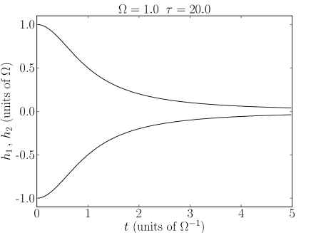
Figure 1: Fields $h_{1}(t)$ and $h_{2}(t)$ for the spin-boson model.

The classical fields have a complicated form, with an initial quadratic decay crossing over to exponential at longer times.  The behavior for $t\gg\tau$ is due to thermal decay while the behavior for $t\ll\tau$ is determined by the cutoff $\Omega$ and is due to fluctuations of the field Breuer and Petruccione (2002).

III.2 Central Spin Model

The central spin Hamiltonian describes a qubit coupled to a bath of nuclear spins.  In the case of free induction decay, the Hamiltonian is

$$H_{CS}=-\frac{1}{2}B\sigma_{z}+H_{int}+H_{hf}$$

where

$$H_{int}=\sum_{i}\omega_{i}J_{i}^{z}+\sum_{i\neq j}b_{ij}\left(J_{i}^{+}J_{j}^{-}-2J_{i}^{z}J_{j}^{z}\right)$$

and

$$H_{hf}=\sigma_{z}\left(\frac{1}{2}\sum_{i}A_{i}J_{i}^{z}+\sum_{i\neq j}\frac{A_{i}A_{j}}{4B}J_{i}^{+}J_{j}^{-}\right).$$

$\omega_{i}$ are the nuclear Zeeman splittings, $b_{ij}$ contain the dipolar interaction, and $A_{i}$ are the hyperfine couplings.  We assume that the initial state is a product state of the qubit and the equilibrium bath state.  For realistic conditions on $\omega_{i}$, $b_{ij}$, and $A_{i}$, the qubit dynamics can be calculated approximately at experimentally relevant time scales Cywiński et al. (2009a, b); Witzel and Das Sarma (2008).  The off-diagonal component of the qubit density matrix is given by $\rho_{10}\left(t\right)=\rho_{10}\left(0\right)D_{cs}\left(t\right)$ where

$$D_{cs}\left(t\right)=\frac{e^{i\arctan\left(\alpha t\right)-iBt}}{\sqrt{1+\alpha^{2}t^{2}}}$$

where $\alpha$ is a complicated function of the parameters of the model.  The explicit dependence is found in Cywiński et al. (2009a) and $\alpha$ determines the relevant time scales since the model is valid only for $\alpha t\ll 1$.  In reference Cywiński et al. (2009a), $1/\alpha\approx 20\,\mu\text{s}$ for a GaAs dot.

The qubit gains an additional phase from the bath interaction.  In terms of $T^{\left(Q\right)}$, we have

$$c_{cs} =\frac{1}{\sqrt{1+\alpha^{2}t^{2}}}\cos\left(\arctan\left(\alpha t\right)-Bt\right)$$

$$s_{cs} =\frac{1}{\sqrt{1+\alpha^{2}t^{2}}}\sin\left(\arctan\left(\alpha t\right)-Bt\right)$$

$$\beta_{cs} =\frac{\alpha t}{\sqrt{1+\alpha^{2}t^{2}}}.$$

Then we can write

$$\Phi_{1} =-Bt+\arctan\left(\alpha t\right)+\arcsin\left(\frac{\alpha t}{\sqrt{1+\alpha^{2}t^{2}}}\right)$$

$$\Phi_{2} =-Bt+\arctan\left(\alpha t\right)-\arcsin\left(\frac{\alpha t}{\sqrt{1+\alpha^{2}t^{2}}}\right)$$

Noting that $\arctan\left(\alpha t\right)=\arcsin\left(\frac{\alpha t}{\sqrt{1+\alpha^{2}t^{2}}}\right)$ and applying Eqs. (15) we get

$$h_{1}^{(cs)}\left(t\right)= \frac{2\alpha}{1+\alpha^{2}t^{2}}$$

and

$$h_{2}^{(cs)}\left(t\right)= 0.$$

This model shows a Lorentzian fall-off of one of the two possible fields but the other one vanishes.  Unlike the spin-boson model, these fields have a non-zero time average which indicates that the central spin noise induces an additional relative phase $\phi$ between the two system states.  Furthermore, if we write the decoherence function as $re^{i\phi}$, for $r,\phi\in\mathbb{R}$ so that $\rho_{10}(t)=\left(\rho_{10}(0)e^{-iBt}\right)\left(r(t)e^{i\phi(t)}\right)$, then the central spin model gives a simple relation between $r$ and $\phi$.  Namely, $r=\cos\phi$ for all values of $t$.

III.3 Quantum Impurity Model

The quantum impurity Hamiltonian is

$$H_{QI}=-\frac{1}{2}B\sigma_{z}+\frac{1}{2}v\left(d^{\dagger}d\right)\sigma_{z}+H_{B}$$

where

$$H_{B}=\epsilon_{0}d^{\dagger}d+\sum_{k}\left(t_{k}c_{k}^{\dagger}d+\text{H.c.}\right)+\sum_{k}\epsilon_{k}c_{k}^{\dagger}c_{k}.$$

$c_{k}^{\dagger}$ creates a reservoir electron and $d^{\dagger}$ creates an impurity electron.  $v$ represents the qubit-impurity coupling strength and $t_{k}$ are the tunneling amplitudes between the impurity and level $k$.  Define the tunneling rate $\gamma=2\pi\sum_{k}\left|t_{k}\right|^{2}\delta(\epsilon_{k}-\epsilon_{0})$.  Assuming an initial product state and an equilibrium bath, this model can be solved via numerically exact techniques Abel and Marquardt (2008).  The off-diagonal components of the qubit density matrix satisfy

$$\rho_{10}\left(t\right)=\rho_{10}\left(0\right)e^{-iBt}D_{qi}(t).$$

Using the numerical methods outlined in Abel and Marquardt (2008), we compute $D(t)=r(t)e^{i\phi(t)}$ for $r(t)>0$.  Applying the method outlined earlier yields

$$\Phi_{i}=-Bt+\phi(t)\pm\cos^{-1}(r(t))$$

and the classical noise source $h^{(qi)}\left(t\right)$ can be calculated using Eqs. (15).  Numerical results are shown in Fig. 2.

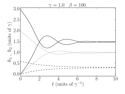
Figure 2: Fields $h_{1}(t)$ and $h_{2}(t)$ for the quantum impurity model. The solid line shows coupling $v=3$ (quantum phase). The dotted line shows $v=2$ (crossover). The dashed line shows $v=0.6$ (classical phase).  Note the oscillatory behavior of the stronger coupling, indicative of coherence oscillation.

This model is of particular interest because it shows a “classical” phase for $v\ll\gamma$ and a “quantum” phase for $v\gg\gamma$ with a crossover region in between.  The quantum phase is characterized by oscillation in the coherence measures such as the visibility.  These oscillations are clearly caused by the oscillations in the noise fields as shown in Fig. 2.  There is, however, nothing quantum about the fields at any value of $v$; they are classical noise sources.

IV Dephasing Of Multiqubit Systems

In this section we generalize the one-qubit dephasing model to a class of multiqubit models that satisfy a transitivity condition.  In contrast to the single-qubit case, there are multiqubit dephasing models that cannot be classically simulated Helm and Strunz (2009).  However, there are multiqubit dephasing models that can be simulated classically and that cannot be reduced to independent qubits.

IV.1 Two-Qubit Dephasing

We will begin with the two-qubit case. The total quantum Hamiltonian again has the form

$$H=H_{S}+H_{B}+H_{SB}.$$

Just as in the single qubit case, we define dephasing models by the condition $\left[H_{S},H_{SB}\right]=0.$  The system Hamiltonian $H_{S}$ can be expanded in the 15 generators of $SU\left(4\right).$  Now we note that the subset of generators having the form $\sigma_{i}\otimes\sigma_{i}$ is mutually commuting.  Consider all models for which these operators commute with the total Hamiltonian.  That is,

$$\left[H,\sigma_{i}\otimes\sigma_{i}\right]=0.$$

for each $i$.  Note that this class of models does not reduce to independent qubits.  For example, the bath could be a set of phonons (or other quantized fields) that modulates an isotropic Heisenberg coupling between two spin 1/2 particles that have a time-independent Ising interaction with each other.

Once again we assume that the system and bath are initially in a product state and that the full density matrix reduces to the system density matrix $\rho$.  Note that since the generators $\sigma_{i}\otimes\sigma_{i}$ are mutually commuting they can be simultaneously diagonalized and the set of eigenstates is equal to the set of maximally entangled Bell states.  In this basis the diagonal elements of $\rho$ are constant, i.e. $\rho_{ii}(t)=\rho_{ii}(0)$. Thus, in this model, the populations of the Bell states remain constant in time. Note that these qubits are entangled and thus are not independent. We will continue to work in this basis for the remainder of the section.

For a classical noise source to simulate the system-bath Hamiltonian and preserve the diagonal elements, each noise source must be diagonal.  Note that in the usual basis, this is equivalent to the condition that each noise term is a linear combination of the generators $\sigma_{i}\otimes\sigma_{i}$.  If this is the case, then the time evolution of the reduced density matrix is given by $\rho_{ij}(t)=r_{ij}(t)\rho_{ij}(0),$ (no summations) and $r_{ij}$ satisfies the conditions $r_{ij}(t)=r_{ji}(t)^{\ast}$, $\left|r_{ij}(t)\right|\leq 1$, and $r_{ii}(t)=r_{ij}(0)=1$.

To simulate this quantum system, we need classical noise sources $H_{\alpha}$ acting with a probability distribution $p(\alpha)$ for $\alpha\in\mathbb{R}$.  The corresponding evolution of the two-qubit density matrix is given by

$$\rho(t)=\int_{-\infty}^{\infty}p(\alpha)U_{\alpha}(t)\rho(0)U_{\alpha}^{\dagger}(t)d\alpha.$$

In our basis of Bell states, the set of valid noise terms $H_{\alpha}$ is simply the set of diagonal matrices. Thus, define the diagonal entries of each $H_{\alpha}$ as $\alpha d_{i}(t)$ so that the set $\left\{H_{\alpha}\right\}$ is characterized by a single parameter, $\alpha$.  This assumption is a particularly simple case.

Time evolution is given by diagonal unitary operators $U_{\alpha}$ with diagonal entries $\exp\left(-i\alpha\theta_{i}(t)\right)$ for

$$\theta_{i}(t)=\int_{0}^{t}d_{i}(t^{\prime})dt^{\prime}.$$

Then the action $U_{\alpha}\rho U_{\alpha}^{\dagger}$ gives

$$\rho_{ij}\rightarrow e^{-i\alpha\gamma_{ij}(t)}\rho_{ij}$$

where $\gamma_{ij}(t)=\theta_{i}(t)-\theta_{j}(t)$.  Applying this result and averaging the result over the probability distribution gives

$$\rho_{ij}(t)= \int_{-\infty}^{\infty}p(\alpha)\rho_{ij}(0)e^{-i\alpha\gamma_{ij}(t)}d\alpha$$

$$= \rho_{ij}(0)\tilde{p}\left(\gamma_{ij}(t)\right)$$ (20)

where $\tilde{p}(t)=\int_{-\infty}^{\infty}p(\alpha)e^{-i\alpha t}d\alpha$.  That is, for the model specified above,

$$r_{ij}(t)=\tilde{p}(\gamma_{ij}(t)).$$ (21)

$r_{ij}$ is just the Fourier transform of the probability distribution $p\left(\alpha\right)$, and we can choose $p\left(\alpha\right)$ as we wish.  This completes the classical description of the process.

The class of quantum systems susceptible to this construction is not very broad: the fact that $\gamma_{ij}$ is a difference of two functions is quite restrictive.  $\gamma_{ij}\left(t\right)$ must satisfy the transitivity condition: $\gamma_{ij}\left(t\right)=\gamma_{ik}\left(t\right)+\gamma_{kj}\left(t\right)$ for all $i,j,k,$ which leads in turn to a restrictive set of conditions on the $r_{ij}(t)$.  Such models are simple enough to construct however, since we only need to specify the $\theta_{i}(t)$ and transitivity is automatically satisfied. However, the transitivity condition limits us to three noise functions $\theta_{i}$ out of a possible six $\gamma_{ij}$.

IV.2 Generalization to Many Qubits

The results for two qubits can be extended to more qubits in a straightforward manner. Let the principal system consist of $n$ qubits.  In the quantum case, we consider the principal system coupled to a bath with evolution governed by a system-bath Hamiltonian $H_{SB}$.

In a system of $n$ qubits, the Pauli operators Nielsen and Chuang (2000) can be formed as the tensor products of 2-qubit Pauli matrices.  Including the identity, there are $4^{n}$ Pauli operators that act on the space of $n$ qubits.  It has been shown Lawrence et al. (2002) that the $4^{n}-1$ Pauli operators (excluding the $2^{n}\times 2^{n}$ identity) can be partitioned into $2^{n}+1$ unique sets of $2^{n}-1$ pairwise commuting operators.  Let $A$ be a subset of the Pauli operators consisting of $2^{n}-1$ commuting operators.  For example, $A$ could be the subset defined by all tensor products of $\sigma_{0}$ and $\sigma_{3}$ (excluding the identity).

The Pauli operators $O_{i}\in A$ are mutually commuting and can be simultaneously diagonalized.  Along with the identity, we have $2^{n}$ independent operators.  Working in a basis such that each $O_{i}$ is diagonal, these operators span the diagonal matrices.  Consider a system-bath Hamiltonian $H_{SB}$ such that

$$\left[H_{SB},O_{i}\right]=0$$

for each $O_{i}$. Since the $O_{i}$ are simultaneously diagonalized, there is no population transfer in the basis of simultaneous eigenstates and it is clear that the above conditions produce dephasing noise and we can define the analogous quantities $r_{ij}(t)$ characterizing the evolution of the principal system. However, as in the two-qubit case, not all of the quantum models satisfying these conditions can be simulated classically.

We can consider a random noise model acting on the principal system specified by $\left\{H_{\alpha}\right\}$ and $p(\alpha)$ with all of the noise terms $H_{\alpha}$ equal to linear combinations of $O_{i}\in A$. Proceeding as in the two-qubit case, define the analogous quantities $\gamma_{ij}(t)$. These $\gamma_{ij}$ remain subject to the transitivity condition $\gamma_{ij}(t)=\gamma_{ik}(t)+\gamma_{kj}(t)$. As in the 2-qubit case, a sufficient condition for classical simulation is that $r_{ij}(t)=\tilde{p}(\gamma_{ij}(t))$. For many qubits, the transitivity condition on $\gamma_{ij}$ becomes increasingly restrictive.  Once again, however, we only need to specify the $\theta_{i}(t)$ in order to construct such a model. With $n$ qubits, this amounts to specifying $2^{n}-1$ degrees of freedom, out of a possible $\left(2^{n-1}\right)\left(2^{n}-1\right)$.

V N-dimensional depolarization

Given a principal quantum system in $N$ dimensions with initial density matrix $\rho_{0}$, the depolarization channel is given by

$$\rho(t)=(1-p(t))\rho_{0}+p(t)\left(\frac{1}{N}\right)I$$

where $p(t)\in[0,1]$ for all $t$ and $p(0)=0$.  $I$ is the $N\times N$ identity matrix.  In this section we drop the subscripts on $\rho.$

A quantum model for depolarization of $n$ $(N=2^{n})$ qubits is given by the Kraus operators $M_{\underline{i}}$ where $\underline{i}=\left(i_{1},i_{2},\ldots,i_{n}\right)$ with $i_{j}\in\left\{0,1,2,3\right\}$

$$M_{\underline{0}}(t)=\sqrt{1-\frac{4^{n}-1}{4^{n}}p(t)}I$$ (22)

and for $\underline{i}\not=\underline{0}$

$$M_{\underline{i}}(t)=\frac{\sqrt{p(t)}}{2^{n}}\left(\sigma_{i_{1}}\otimes\sigma_{i_{2}}\otimes\cdots\otimes\sigma_{i_{n}}\right).$$ (23)

Then

$$\rho(t)=\sum_{\underline{i}}M_{\underline{i}}\rho_{0}M_{\underline{i}}^{\dagger}$$ (24)

holds for $\rho(t)$ defined above Nielsen and Chuang (2000).

We now present a classical model for depolarization in arbitrary dimension.  Consider the unitary group $SU(N)$. $\ N\$need not be a power of 2, so the following construction holds not only for qubit arrays, but also for qudits. Each time-independent $U\in SU(N)$ can be expanded in terms of its eigenvectors $\left|j\right\rangle$ as

$$U=\sum_{j}e^{-id_{j}}\left|j\right\rangle\left\langle j\right|$$

with $d_{j}\in\left(-\pi,\pi\right]$.  For a fixed $U$, define $H_{U}$ as

$$H_{U}=\sum_{j}d_{j}\left|j\right\rangle\left\langle j\right|$$

so that

$$U=\left.e^{-iH_{U}t}\right|_{t=1}.$$

Note that each $H_{U}$ can be expanded as

$$H_{U}=\sum_{r}h_{r}\lambda_{r}$$

where $h_{r}$ are real and $\lambda_{r}$ are the generators of $SU(N)$. Then consider the Hamiltonian defined by the set $\left\{H_{U}\right\}$ with the probability distribution equal to the uniform distribution in Haar measure over $SU(N)$.  For convenience, choose

$$\int_{SU(N)}dU=1$$

where the integral is taken with respect to the Haar measure.  Time evolution is then given by

$$\rho(t)=\int_{SU(N)}e^{-iH_{U}t}\rho(0)e^{iH_{U}t}dU.$$ (25)

We need to show that this time evolution is purely depolarizing. Consider an arbitrary unitary transformation $V$ such that

$$V\rho_{0}V^{\dagger}=\rho_{0}.$$

Then we can write that

$$\rho(t)=\int_{SU(N)}e^{-iH_{U}t}V\rho_{0}V^{\dagger}e^{iH_{U}t}dU$$

from which we can easily obtain

$$V^{\dagger}\rho(t)V=\int_{SU(N)}V^{\dagger}e^{-iH_{U}t}V\rho_{0}V^{\dagger}e^{iH_{U}t}VdU.$$

Since the above integral runs over the entire unitary group $SU(N)$, conjugation by $V$ simply amounts to a reparameterization of the integral.  Thus, we can write

$$V^{\dagger}\rho(t)V=\int_{SU(N)}e^{-iH_{U}t}\rho_{0}e^{iH_{U}t}dU=\rho(t).$$ (26)

Hence, any rotation leaving the initial polarization vector fixed must also leave $\rho(t)$ fixed, and the polarization vector of $\rho(t)$ must be parallel to that of $\rho_{0}$.

Now, consider the case $t=1$.  From our initial definition of $H_{U}$, we see that

$$\rho(t=1)=\int_{SU(N)}U\rho_{0}U^{\dagger}dU.$$

Further consider an arbitrary unitary operator $W$. Then conjugation gives

$$W\rho(t =1)W^{\dagger}=\int_{SU(N)}WU\rho_{0}U^{\dagger}W^{\dagger}dU$$

$$=\int_{SU(N)}U\rho_{0}U^{\dagger}dU$$

since if $U$ runs over the entire unitary group than so does $WU$.  Thus, we see that

$$W\rho(t=1)W^{\dagger}=\rho(t=1).$$

Since this holds for arbitrary unitary operator $W$, we must have that $\rho(1)$ is proportional to the identity.  Thus, $\rho(1)$ is the totally mixed state and we see that the model presented is indeed a depolarizing channel.

For the single qubit ($N=1$) case, the integral can be evaluated explicitly.  Without loss of generality, assume that the initial qubit state is specified by

$$\rho(t=0)=\frac{1}{2}\left(I+\sigma_{z}\right).$$

Then

$$\rho(t)=\frac{1}{2}\left(I+n_{z}(t)\sigma_{z}\right).$$

The integration in Eq. 25 reduces to an integral over the $3$-sphere $S^{3}$.  It can be evaluated explicitly and one finds

$$n_{z}(t)=\frac{1}{3}+\frac{\sin(2\pi t)}{3\pi(t-t^{3})}.$$ (27)

This expression indeed satisfies $n_{z}(t=0)=1$ and $n_{z}(t=1)=0$.  Somewhat surprisingly, this function has a root near $t=0.77$ and has a limiting value of $1/3$ as $t\rightarrow\infty$.  Because of the unexpected root, proper depolarization behavior ends before $t=1$, however a simple reparameterization of time and the corresponding redefinition of noise terms $H_{\alpha}$ allows for arbitrary depolarizing behavior.  The graph of $n_{z}(t)$ is shown in Fig. 3.

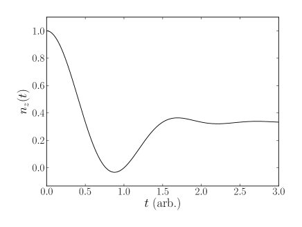
Figure 3: The $z$ component of the Bloch vector as a function of time for single qubit classical depolarization.  Note that proper depolarization ends at the first root ($t\approx 0.77$).

In this classical model the noise histories belong to an uncountably infinite set.  It is also possible to construct a classical depolarization model using a finite set of histories.  The Clifford group $C\left(N\right)$ is a subgroup of $SU\left(N\right)$ defined as the stabilizer group of the Pauli group; the latter consists of tensor products of the Pauli matrix multiplied by the units of the complex numbers.  It has been shown that $C\left(N\right)$ is a unitary 2-design, meaning that averages over the Clifford group of polynomial expressions of degree less than or equal to two (such as $\rho_{0})$ are equal to uniform averages over the Haar measure Dankert et al. (2009); Gross et al. (2007); Seymour and Zaslavsky (1984).  This means that the above derivation of the depolarizing evolution may be repeated with the substitution

$$\int_{SU(N)}f\left(U\right)dU\rightarrow\frac{1}{\left|C\left(N\right)\right|}\sum_{C}f\left(C\right).$$

Since the members of $C\left(N\right)$ are unitary, evolution of $\rho$ according to

$$\frac{1}{\left|C\left(N\right)\right|}\sum_{U\in C}C\rho C^{{\dagger}}$$

is a RC evolution.  The construction of the equivalent depolarizing quantum system-bath model then proceeds as in Eqs. 16-18.

VI Conclusion

We have shown how to construct classical simulations of decoherence arising from the interactions of a single qubit and an external bath for the pure dephasing case.  We demonstrated that the noise functional takes on the particularly simple form of two uniformly distributed random unitary evolutions and gave the explicit expression for the corresponding Hamiltonian fields.  We offered exact results of the calculation of these fields for the spin-boson model, approximate results for the central spin model, and numerically exact results for the quantum impurity model.

Classical simulation of quantum noise acting on multiple qubits and qudits is also possible in certain cases. For two interacting qubits, we showed that the simulation is possible if the interaction is sufficiently simple and we gave the corresponding classical noise model.  We demonstrated that the depolarization channel can be simulated classically for a state space of arbitrary dimension, using well-known properties of the Clifford group.

Philosophically, it is surprising that classical simulation is mainly possible when the decoherence arises from phase randomness of quantum states and is more difficult when the decoherence comes from randomness in the population of those states, since phase is a characteristic of quantum mechanics that is not shared with classical mechanics, while the concept of population is common to both.