Testing chemical composition of highest energy comic rays

Abstract

We study basic characteristics of distributions of the depths of shower maximum in air showers caused by cosmic rays with the highest energies. The consistency between their average values and widths, and their energy dependences are discussed within a simple phenomenological model of shower development independently of assumptions about detailed features of high–energy interactions. It is shown that reliable information on primary species can be derived within a partition method. We present examples demonstrating implications for the changes in mass composition of primary cosmic rays.

1 Introduction

Knowledge of the mass distribution of cosmic rays (CR) and of its energy evolution can provide useful information about CR acceleration mechanisms and propagation through the galactic and extragalactic space. Measurements and subsequent analysis of the mass composition of ultra–high energy cosmic ray (UHECR) primaries are of particular importance. Corresponding observables can help to understand their typical spectral features, the ankle at about $4\leavevmode\nobreak\ {\rm EeV}$ and the steep flux suppression at energies above $30\leavevmode\nobreak\ {\rm EeV}$. In addition, their knowledge makes searches for the CR sources much easier.

In seeking for the mass of UHECR particles, the development of extensive air showers (EAS) of secondary particles created in the Earth atmosphere is usually examined. The mean penetration depth in the atmosphere at which the shower of secondary particles reaches its maximum number, $\langle X_{\rm max}\rangle$, and $\sigma_{\rm max}=\sigma(X_{\rm max})$, the square root of its variance, are widely used. Recent results presented by the Auger collaboration indicate a transition from lighter to heavier primaries at the ankle region [1, 2]. The HiRes collaboration achieved a different conclusion. Its analysis based on the truncated fluctuation widths speaks in favor of very light primaries at the highest energies [3].

Based on widely accepted empirical characteristics of the energy evolution of the mean depth of shower maximum and its variance, we present a method in which reasonable inferences about the partition of the primary CR mass are naturally achieved. Utilizing a generalized Heitler model [4, 5], two illustrative examples are presented. We make use of the recently measured value of the $p$–air cross section [6] and try intentionally to account for the details of EAS development independently of assumptions about detailed features of hadronic interactions.

2 Air shower model

Let us assume that a CR shower maximum $X_{\rm max}$ is measured when a UHECR particle with a mass $A$ hits the upper part of the Earth atmosphere. In the following we will treat these two quantities as dependent random variables, $X_{\rm max}=X_{\rm max}(A)$. Adopting superposition assumptions [5], the mean depth of shower maximum provided air showers are initiated by primaries of the mass $A$ depends on the shower energy $E$ as [4, 5]

$$\langle X_{\rm max}\mid A\rangle=C+D\leavevmode\nobreak\ {\rm Log}\left(\frac{E}{E_{0}A}\right).$$ (1)

Here, $D=\frac{{\rm d}\langle x_{\rm max}\rangle}{{\rm d}{\rm Log}E}$ is the proton elongation rate [5], where $\langle x_{\rm max}\rangle=\langle X_{\rm max}\mid A=1\rangle$ is the proton mean depth of shower maximum, and $C=\langle x_{\rm max}\rangle(E_{0})$ is a constant proton mean depth of maximum at a reference energy of $E_{0}$. In the same line, the conditional variance of the depth of maximum is

$$\sigma^{2}(X_{\rm max}\mid A)=\sigma_{\rm fr}^{2}+\sigma_{\rm sh}^{2},$$ (2)

where $\sigma_{\rm fr}^{2}=\sigma_{\rm fr}^{2}(A,E)$ is the variance of the depth where the first interaction of the CR primary takes place and $\sigma_{\rm sh}^{2}=\sigma_{\rm sh}^{2}(A,E)$ assigns the variance of the depth of shower maximum associated with its subsequent development [5]. Then, the total mean and total variance of the depth of shower maximum at a given energy $E$ that are to be confronted with measurements, are respectively

$$\langle X_{\rm max}\rangle=\langle\langle X_{\rm max}\mid A\rangle\rangle=\langle x_{\rm max}\rangle-d\langle\ln A\rangle,$$ (3)

and

$$\sigma^{2}_{\rm max}=\sigma^{2}(X_{\rm max})=\langle\sigma_{\rm fr}^{2}\rangle+\langle\sigma_{\rm sh}^{2}\rangle+d^{2}\sigma_{\ln{\rm A}}^{2},$$ (4)

where $D=d\ln 10$ was inserted and the law of total variance was used, i.e.$\sigma^{2}_{\rm max}=\langle\sigma^{2}(X_{\rm max}\mid A)\rangle+\sigma^{2}(\langle X_{\rm max}\mid A\rangle)$, see e.g. Ref. [7]. Except for $\langle x_{\rm max}\rangle$, the other mean values written on the right hand sides in Eqs.(3) and (4) are calculated over mass numbers of primary CR particles.

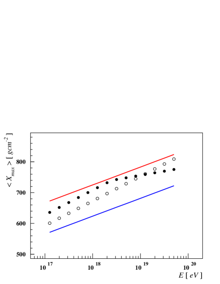
Figure 1: Two hypothetical examples of mean values of $\langle X_{\rm max}\rangle$ are shown as functions of energy. Black empty points are for the constant elongation rate. Black full points show the elongation rate with a break as indicated by a magenta arrow. MC predictions of $\langle X_{\rm max}\rangle$ for proton and iron primaries are illustrated by red and blue line, respectively.

3 Partition problem

To examine the mass composition we utilize the partition method described briefly in Appendix A. To this end, we use two $A$–dependent constrains, $F_{1}(A)=d\ln A$ and $F_{2}(A)=d^{2}\ln^{2}A+\sigma_{\rm fr}^{2}+\sigma_{\rm sh}^{2}$, respectively. Their average values are given by the available experimental information contained in the $X_{\rm max}$ measurements. They are directly connected to the total sample mean, $\langle X_{\rm max}\rangle$, and to the total sample variance of $X_{\rm max}$, $\sigma^{2}_{\rm max}$, measured at given energy. The aforementioned constrains are written as

$$\langle F_{1}\rangle=d\langle\ln A\rangle=Q_{\rm max},$$ (5)

$$\langle F_{2}\rangle=d^{2}\langle\ln^{2}A\rangle+\langle\sigma_{\rm fr}^{2}\rangle+\langle\sigma_{\rm sh}^{2}\rangle=\sigma^{2}_{\rm max}+Q_{\rm max}^{2},$$ (6)

where $Q_{\rm max}=\langle x_{\rm max}\rangle-\langle X_{\rm max}\rangle$.

In the partition method, the probability distribution of the mass number is dictated by the maximum–entropy principal as described in Appendix A. Knowing the total mean and variance at given energy, $\langle X_{\rm max}\rangle$ and $\sigma^{2}_{\rm max}$, the form of this distribution is given by Eq.(10) with two Lagrangian multipliers deduced numerically in such a way that the two constrains written in Eqs.(5) and (6) are satisfied.

In this study, the proton mean depth of shower maximum $C=\langle x_{\rm max}\rangle(E_{0})$ at a reference energy of $E_{0}$ and the energy independent proton elongation rate $D=d\ln 10$ are only two free parameters.

The $A$–dependence of the depth of shower maximum is given by the Heitler conjecture, see Eq.(1). For other mass dependent terms we use simple phenomenological arguments described in Appendix B. The variance of the depth of the first interaction, $\sigma_{\rm fr}^{2}=\sigma_{\rm fr}^{2}(A,E)$, is deduced from the measured $p$–air cross section and its extrapolated energy dependence [6]. The variance of the depth of shower maximum connected with the shower development, $\sigma_{\rm sh}^{2}=\sigma_{\rm sh}^{2}(A,E)$, is inferred from basic characteristics of underlying interaction processes. Let us stress that other parametrizations of the EAS $A$–dependent terms, different from that ones introduced in Appendix B, can be adopted in our treatment.

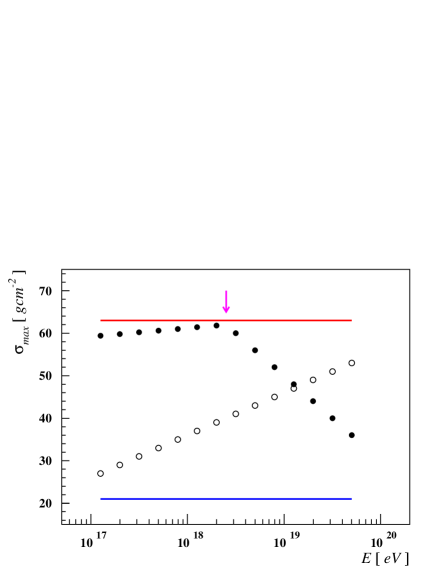
Figure 2: Square roots of variances $\sigma_{\rm max}$ used in two illustrative example are shown as functions of energy. The constant elongation rate (black empty points) and the elongation rate with a break (black full points) are shown, see also Fig.1. Red and blue lines illustrate MC predictions of $\sigma_{\rm max}$ for proton and iron primaries, respectively.

4 Illustrative examples

We successfully applied the maximum–entropy method for a number of artificially chosen examples with average shower characteristics resembling their measured energy evolution. Within the partition method, we decomposed these observables into different sets of primary masses assuming different parametrization of the mean depth of shower maximum and its variance. In the following, we present results of two of these hypothetical examples.

In the first example, we used the mean depth of shower maximum with a constant elongation rate and a logarithmically increasing square root of the depth variance with energy. These shower statistics, displayed in Figs.1 and 2 as black empty points, were parametrized by

$$\frac{\langle X_{\rm max}\rangle(E)-X_{0}}{D_{0}}=\frac{\sigma_{\rm max}(E)-\sigma_{0}}{s_{0}}={\rm Log}\left(\frac{E}{E_{0}}\right),$$ (7)

where $X_{0}=673\leavevmode\nobreak\ {\rm gcm^{-2}}$ and $\sigma_{0}=36\leavevmode\nobreak\ {\rm gcm^{-2}}$ are shower statistics at a reference energy of $E_{0}=1\leavevmode\nobreak\ {\rm EeV}$, and parameters $D_{0}=80\leavevmode\nobreak\ {\rm gcm^{-2}}$ and $s_{0}=10\leavevmode\nobreak\ {\rm gcm^{-2}}$. An energy interval ${\rm Log}(E/{\rm eV})\in\langle 17.1,19.7\rangle$ with $14$ equidistant values ($\Delta{\rm Log}(E/{\rm EeV})=0.2$) was assumed.

In the following calculations, we tried to decompose the mass composition represented by the shower statistics, $\langle X_{\rm max}\rangle(E)$ and $\sigma_{\rm max}(E)$, into four pieces corresponding to primary species generating underlying CR showers. Namely, we assumed proton primaries ($A=1$), and helium ($A=4$), nitrogen ($A=14$) and iron ($A=56$) nuclei. In the first step, we solved the partition problem numerically treating the two unknown quantities, $C$ and $D$ introduced in Eq.(1), as free parameters. This way, we obtained a two–dimensional domain where maximum–entropy solutions exist. In the second step, we performed the partition analysis with parameters $C=(730-740)\leavevmode\nobreak\ {\rm gcm^{-2}}$ and $D=(56-60)\leavevmode\nobreak\ {\rm gcm^{-2}}$ that provided us the best solutions of the partition problem.

Our results are summarized in top panels in Figs.3 and 4. In the top panel in Fig.3, decomposition probabilities of hypothetical shower statistics are depicted as functions of energy. The widths of colored bands correspond to aforementioned uncertainties in parameters $C$ and $D$. The mean and variance of logarithmic mass are depicted in the top panel in Fig.4. Both characteristics give the expected trends with steeply falling $\langle\ln A\rangle$ and growing up variance $\sigma_{\rm\ln A}^{2}$ with the increasing energy. Large uncertainties of heavier primaries at energies where small values of $\langle X_{\rm max}\rangle$ and $\sigma_{\rm max}$ were chosen are salient features of our treatment.

In the second example, we tried to analyze hypothetical shower statistics that resemble real data as measured by the Auger detector [1, 2]. To this end, we prepared the input data, $\langle X_{\rm max}\rangle(E)$ and $\sigma_{\rm max}(E)$, with breaks as depicted in Figs.1 and 2 by black full points. For the energy evolution of the mean depth of shower maximum we adopted an elongation rate of $D_{0}=80\leavevmode\nobreak\ {\rm gcm^{-2}}$ for energies ${\rm Log}(E/{\rm eV})<18.4$ and $D_{0}=27\leavevmode\nobreak\ {\rm gcm^{-2}}$ above this energy with $X_{0}=708\leavevmode\nobreak\ {\rm gcm^{-2}}$, see Eq.(7). For the evolution of the variance we took $s_{0}=2\leavevmode\nobreak\ {\rm gcm^{-2}}$ for ${\rm Log}(E/{\rm eV})<18.4$, $s_{0}=-20\leavevmode\nobreak\ {\rm gcm^{-2}}$ otherwise, and $\sigma_{0}=61.2\leavevmode\nobreak\ {\rm gcm^{-2}}$.

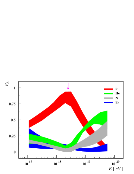
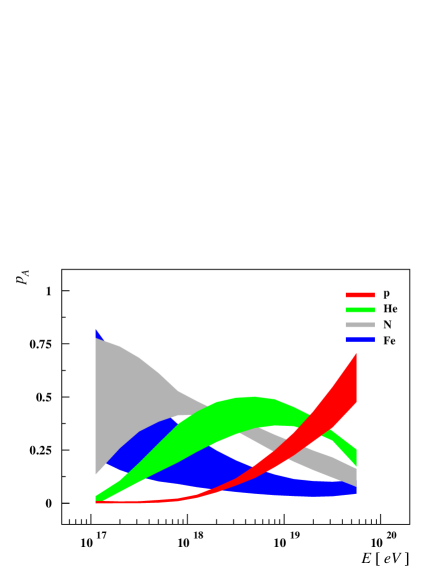
Figure 3: Primary mass partition is depicted as a function of energy. We used hypothetical shower characteristics for the constant elongation rate (top panel) and the elongation rate with a break (bottom panel) as shown in Figs.1 and 2. Red, green, gray and blue bands are for proton, helium, nitrogen and iron primaries. Their widths correspond to uncertainties of parameters $C=\langle x_{\rm max}\rangle(E_{0})$ and $D$.

We adopted the same set of primary species that generated showers with statistics under considerations, $p$, ${\rm He}$, ${\rm N}$ and ${\rm Fe}$. We examined a domain for two free parameters giving us $C=(720-730)\leavevmode\nobreak\ {\rm gcm^{-2}}$ and $D=(54-62)\leavevmode\nobreak\ {\rm gcm^{-2}}$ ranges where the best maximum–entropy solutions exist.

The resultant mass decomposition is displayed in the bottom panel in Fig.3. The mean value and variance of logarithmic mass are depicted in the bottom panel in Fig.4. Also in this hypothetical example we obtained reasonable solutions. The chosen breaks in shower statistics are well visible in the energy evolution of the resultant partition probabilities. The lightest component, driven up to the chosen break dies out rapidly after it reaches its maximum value near the break at ${\rm Log}(E/{\rm eV})=18.4$. Interestingly, the proton–iron mixture is not able to explain the chosen energy evolution of shower statistics. For a reasonable description intermediate mass nuclei are necessary.

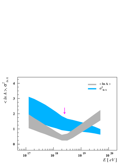
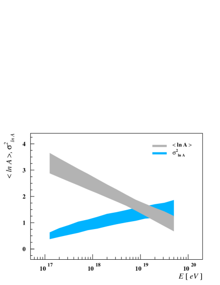
Figure 4: Mean logarithms of the mass number (gray) and their variances (blue) are plotted as functions of energy. Hypothetical shower characteristics for the constant elongation rate (top panel) and the elongation rate with a break (bottom panel) depicted in Figs.1 and 2 are used. Widths of plotted statistics correspond to uncertainties of parameters $C=\langle x_{\rm max}\rangle(E_{0})$ and $D$.

5 Conclusions

We used the well justified maximum–entropy method to deduce the partition of the mass of CR primaries from the hypothetical characteristics of the EAS development that they initiated. This method combines simple properties of the generalized Heitler model, multiplication characteristics of air showers and the measured $p$–air cross section. It is independent of details on hadronic interactions.

The partition method enables us to establish a reasonable connection between the mean value of the logarithmic primary mass number, its variance and other observables as well. The resultant decomposition of the mass distribution describes what we know from experiment as effectively as possible provided the selected model of the shower evolution holds. Let us finally stress that the consistency of deduced quantities, as interpreted in the Heitler reasoning, is emphasized rather then questioned within the partition method.

Appendix A Partition formalism

Let us assume that the quantity $A$ is capable to take $n$ discrete values $A=1,\dots,n$. Corresponding probabilities $p_{\rm A}$ are not known, however. Only a set of $r$ expectation values of the functions $F_{i}(A)$, $i=1,\dots,r$, $r<n$, is measured. For setting up a probability distribution which satisfies the given data, the least biased estimate possible on the basis of partial knowledge is used. This method, known as the maximum–entropy principle, is widely used in statistical mechanics [8]; for its statistical background see e.g. [7].

Here, Shannon entropy [8]

$$S=-k\sum\limits_{A=1}^{n}p_{\rm A}\ln p_{\rm A},$$ (8)

where $k$ is a positive constant, is adopted as an information measure of the amount of uncertainty in the probability distribution $p_{\rm A}$ of the quantity $A$. This distribution is determined as the one that maximizes entropy $S$ in Eq.(8) subject to $r$ constraints, $F_{i}(A)$, $i=1,\dots,r$, given their averages that represent whatever experimental information one has, and subject to the normalization condition

$$\langle F_{i}\rangle=\sum\limits_{A=1}^{n}p_{\rm A}F_{i}(A),\quad i=1,\dots,r,\qquad\sum\limits_{A=1}^{n}p_{\rm A}=1.$$ (9)

Then, the resultant distribution describes what we know about the quantity $A$ from experiment without assuming anything else [8].

In making inferences on the basis of partial information, the maximum–entropy probability distribution that maximizes Shannon entropy in Eq.(8) subject to the experimental constraints written in Eq.(9) is given by [8]

$$p_{\rm A}=Z^{-1}e^{-\left[\lambda_{1}F_{1}(A)+\dots+\lambda_{r}F_{r}(A)\right]},$$ (10)

with the partition function written

$$Z(\lambda_{1},\dots,\lambda_{r})=\sum\limits_{A=1}^{n}e^{-\left[\lambda_{1}F_{1}(A)+\dots+\lambda_{r}F_{r}(A)\right]},$$ (11)

and with Lagrangian multipliers $\lambda_{i}$, $i=1,\dots,r$, to be determined. The resultant probability distribution obtained in this process is spread out as widely as possible without contradicting the available experimental information.

Appendix B Shower variances

In our method, the depth of shower maximum caused by a primary proton with energy $E$ is assumed to be [5]

$$\langle x_{\rm max}\rangle(E)\approx\lambda(E)+X\leavevmode\nobreak\ \ln\left(\frac{\kappa E}{2M\epsilon}\right),$$ (12)

where $\lambda(E)$ is the average interaction length for inelastic $p$–air collisions, $X\approx 37\leavevmode\nobreak\ {\rm gcm^{-2}}$ is the radiation length in air, $\epsilon\approx 84\leavevmode\nobreak\ {\rm MeV}$ denotes the critical energy in air, $\kappa$ is the elasticity of the first interaction and $M$ assigns its multiplicity. This relationship is well documented by physical arguments and by MC simulations as well. It can also be derived as an approximate solution of Yule birth process.

For the variance of the depth of the first interaction we have adopted the measured $p$–air cross section at a center of mass energy of $\sqrt{s}=57\leavevmode\nobreak\ {\rm TeV}$ [6]. Relying upon a smooth extrapolation from accelerator measurements, and in agreement with model predictions, here we used a parametrization $\Sigma_{\rm p-Air}\approx\left[500+50\leavevmode\nobreak\ {\rm Log}(E/{\rm EeV})\right]\leavevmode\nobreak\ {\rm mb}$. Within a naive model, the variance of the depth of the first interaction is then approximately

$$\sigma_{\rm fr}^{2}=\sigma_{\rm fr}^{2}(A,E)\approx A^{-\alpha}\xi(E)\sigma_{\rm fr,0}^{2},$$ (13)

where $A$ assigns the mass number of a primary CR particle and $\alpha$ is a constant index. The variance of the depth of shower maximum caused by the proton primary at the reference energy of $E_{0}=1\leavevmode\nobreak\ {\rm EeV}$, $\sigma_{\rm fr,0}\approx 46\leavevmode\nobreak\ {\rm gcm^{-2}}$, is deduced from the measured $p$–air cross section as well as a function $\xi(E)\approx 1-0.2\leavevmode\nobreak\ {\rm Log}(E/{\rm EeV})$. The $A$–dependent term in Eq.(13) accounts for details of the first interaction given by individual nucleon–nucleon interactions and subsequent nuclear fragmentation [5]. A statistical treatment assuming a subset of interacting nucleons supplemented by simple geometrical arguments gives approximately $\alpha\approx\frac{2}{3}$. In our analysis, we have examined values of $\alpha\approx 0.3-3.0$ yielding slightly different results that were negligible if uncertainties of other parameters were taken into account.

Assuming an experimental value $\sigma_{\rm max}\approx 60\leavevmode\nobreak\ {\rm gcm^{-2}}$ at about $1\leavevmode\nobreak\ {\rm EeV}$ [1, 2], and predominantly proton primaries, we estimated the variance of the depth of shower maximum in the subsequent shower development by

$$\sigma_{\rm sh}^{2}=\sigma_{\rm sh}^{2}(A,E)\approx A^{-1}\sigma_{\rm sh,0}^{2},$$ (14)

where $\sigma_{\rm sh,0}\approx 38\leavevmode\nobreak\ {\rm gcm^{-2}}$. The $A$–dependence of the shower variance is given by fluctuations in multiplicity $M$ and elasticity $\kappa$ of the first (or main) interaction. Assuming a model in Eq.(12), the corresponding variances caused by primary protons are $\sigma_{\rm M,0}^{2}\approx X^{2}M^{-2}\sigma_{\rm M}^{2}$, $\sigma_{\rm\kappa,0}^{2}\approx X^{2}\kappa^{-2}\sigma_{\rm\kappa}^{2}$, giving $\sigma_{\rm sh,0}^{2}=\sigma_{\rm M,0}^{2}+\sigma_{\rm\kappa,0}^{2}$. In a naive superposition model [5], the variance of the total multiplicity of $k$ nucleons participating in the main interaction with an average multiplicity $\overline{M}$ is $\sigma^{2}(k\overline{M})=k^{2}A^{-1}\sigma_{\rm M}^{2}$, and similarly for an average elasticity, $\sigma^{2}(\overline{\kappa})=A^{-1}\sigma_{\rm\kappa}^{2}$, supporting Eq.(14).

Acknowledgment: This work was supported by the grants MSMT–CR LG13007 and MSM0021620859 of the Ministry of Education, Youth and Sports of the Czech Republic. The authors would like to thank Petr Travnicek for his help and support.

References

- [1] J.Abraham et al., Phys.Rev.Lett. 104 (2010) 091101.
- [2] P.Facal and Pierre Auger Collaboration, Proc. 32th Int.Conf.Cosmic Rays, Beijing, Vol.2, 2011, p.105.
- [3] R.U.Abbasi et al., Phys.Rev.Lett. 104 (2010) 161101.
- [4] J. Matthews, Astropart. Phys. 22 (2005) 387.
- [5] K.–H.Kampert, M.Unger, Astropart.Phys. 35 (2012) 660.
- [6] P.Abreu, et al., Phys.Rev.Lett. 109 (2012) 062002.
- [7] R.C.Rao, Linear Statistical Inference and Its Applications, John Willey & Sons, 1973.
- [8] E.T.Jaynes, Phys.Rev. 106 (1957) 620.