Asymptotically Normal and Efficient Estimation of Covariate-Adjusted Gaussian Graphical Model

Abstract

A tuning-free procedure is proposed to estimate the covariate-adjusted Gaussian graphical model. For each finite subgraph, this estimator is asymptotically normal and efficient. As a consequence, a confidence interval can be obtained for each edge. The procedure enjoys easy implementation and efficient computation through parallel estimation on subgraphs or edges. We further apply the asymptotic normality result to perform support recovery through edge-wise adaptive thresholding. This support recovery procedure is called ANTAC, standing for Asymptotically Normal estimation with Thresholding after Adjusting Covariates. ANTAC outperforms other methodologies in the literature in a range of simulation studies. We apply ANTAC to identify gene-gene interactions using an eQTL dataset. Our result achieves better interpretability and accuracy in comparison with CAMPE.

Keywords: Sparsity, Precision matrix estimation, Support recovery, High-dimensional statistics, Gene regulatory network, eQTL

1 Introduction

Graphical models have been successfully applied to a broad range of studies that investigate the relationships among variables in a complex system. With the advancement of high-throughput technologies, an unprecedented amount of features can be collected for a given system. Therefore, the inference with graphical models has become more challenging. To better understand the complex system, novel methods under high dimensional setting are extremely needed. Among graphical models, Gaussian graphical models have recently received considerable attention for their applications in the analysis of gene expression data. It provides an approach to discover and analyze gene relationships, which offers insights into gene regulatory mechanism. However gene expression data alone are not enough to fully capture the complexity of gene regulation. Genome-wide expression quantitative trait loci (eQTL) studies, which simultaneously measure genetic variation and gene expression levels, reveal that genetic variants account for a large proportion of the variability of gene expression across different individuals (?). Some genetic variants may confound the genetic network analysis, thus ignoring the influence of them may lead to false discoveries. Adjusting the effect of genetic variants is of importance for the accurate inference of genetic network at the expression level. A few papers in the literature have considered to accommodate covariates in graphical models. See, for example, ?, ? and ? introduced Gaussian graphical model with adjusted covariates, and ? introduced additional covariates to Ising models.

This problem has been naturally formulated as joint estimation of the multiple regression coefficients and the precision matrix in Gaussian settings. Since it is widely believed that genes operate in biological pathways, the graph for gene expression data is expected to be sparse. Many regularization-based approaches have been proposed in the literature. Some use a joint regularization penalty for both the multiple regression coefficients and the precision matrix and solve iteratively (?; ?; ?). Others apply a two-stage strategy: estimating the regression coefficients in the first stage and then estimating the precision matrix based on the residuals from the first stage. For all these methods, the thresholding level for support recovery depends on the unknown matrix $l_{1}$ norm of the precision matrix or an irrepresentable condition on the Hessian tensor operator, thus those theoretically justified procedures can not be implemented practically. In practice, the thresholding level is often selected through cross-validation. When the dimension $p$ of the precision matrix is relatively high, cross-validation is computationally intensive, with a jeopardy that the selected thresholding level is very different from the optimal one. As we show in the simulation studies presented in Section 5, the thresholding levels selected by the cross-validation tend to be too small, leading to an undesired denser graph estimation in practice. In addition, for current methods in the literature, the thresholding level for support recovery is set to be the same for all entries of the precision matrix, which makes the procedure non-adaptive.

In this paper, we propose a tuning free methodology for the joint estimation of the regression coefficients and the precision matrix. The estimator for each entry of the precision matrix or each partial correlation is asymptotically normal and efficient. Thus a P-value can be obtained for each edge to reflect the statistical significance of each entry. In the gene expression analysis, the P-value can be interpreted as the significance of the regulatory relationships among genes. This method is easy to implement and is attractive in two aspects. First, it has the scalability to handle large datasets. Estimation on each entry is independent and thus can be parallelly computed. As long as the capacity of instrumentation is adequate, those steps can be distributed to accommodate the analysis of high dimensional data. Second, it has the modulability to estimate any subgraph with special interests. For example, biologists may be interested in the interaction of genes play essential roles in certain biological processes. This method allows them to specifically target the estimation on those genes. An R package implementing our method has been developed and is available on the CRAN website.

We apply the asymptotic normality and efficiency result to do support recovery by edge-wise adaptive thresholding. This rate-optimal support recovery procedure is called ANTAC, standing for Asymptotically Normal estimation with Thresholding after Adjusting Covariates. This work is closely connected to a growing literature on optimal estimation of large covariance and precision matrices. Many regularization methods have been proposed and studied. For example, Bickel and Levina (?; ?) proposed banding and thresholding estimators for estimating bandable and sparse covariance matrices respectively and obtained rate of convergence for the two estimators. See also ? and ?. ? established the optimal rates of convergence for estimating bandable covariance matrices. ? and ? obtained the minimax rate of convergence for estimating sparse covariance and precision matrices under a range of losses including the spectral norm loss. Most closely related to this paper is the work in ? where fundamental limits were given for asymptotically normal and efficient estimation of sparse precision matrices. Due to the complication of the covariates, the analysis in this paper is more involved.

We organize the rest of the paper as follows. Section 2 describes the covariate-adjusted Gaussian graphical model and introduces our novel two-step procedure. Corresponding theoretical studies on asymptotic normal distribution and adaptive support recovery are presented in Sections 3-4. Simulation studies are carried out in Section 5. Section 6 presents the analysis of eQTL data. Proofs for theoretical results are collected in Section 7. We collect a key lemma and auxiliary results for proving the main results in Section 8 and Appendix 9.

2 Covariate-adjusted Gaussian Graphical Model and Methodology

In this section we first formally introduce the covariate-adjusted Gaussian graphical model, and then propose a two-step procedure for estimation of the model.

2.1 Covariate-adjusted Gaussian Graphical Model

Let $\left(X^{(i)},Y^{(i)}\right)$, $i=1,...,n$, be i.i.d. with

$$Y^{(i)}=\Gamma_{p\times q}X^{(i)}+Z^{\left(i\right)}\text{,}$$ (1)

where $\Gamma$ is a $p\times q$ unknown coefficient matrix, and $Z^{\left(i\right)}$ is a $p-$dimensional random vector following a multivariate Gaussian distribution $N\left(0,\Omega^{-1}\right)$ and is independent of $X^{(i)}$. For the genome-wide expression quantitative trait studies, $Y^{(i)}$ is the observed expression levels for $p$ genes of the $i-$th subject and $X^{(i)}$ is the corresponding values of $q$ genetic markers. We will assume that $\Omega$ and $\Gamma_{p\times q}$ are sparse. The precision matrix $\Omega$ is assumed to be sparse partly due to the belief that genes operate in biological pathways, and the sparseness structure of $\Gamma$ reflects the sensitivity of confounding of genetic variants in the genetic network analysis.

We are particularly interested in the graph structure of random vector $Z^{\left(i\right)}$, which represents the genetic networks after removing the effect of genetic markers. Let $G=(V,E)$ be an undirected graph representing the conditional independence relations between the components of a random vector $Z^{\left(1\right)}=(Z_{11},\dotsc,Z_{1p})^{T}$. The vertex set $V=\{V_{1},\dotsc,V_{p}\}$ represents the components of $Z$. The edge set $E$ consists of pairs $(i,j)$ indicating the conditional dependence between $Z_{1i}$ and $Z_{1j}$ given all other components. In the genetic network analysis, the following question is fundamental: Is there an edge between $V_{i}$ and $V_{j}$? It is well known that recovering the structure of an undirected Gaussian graph $G=\left(V,E\right)$ is equivalent to recovering the support of the population precision matrix $\Omega=\left(\omega_{ij}\right)$ of the data in the Gaussian graphical model. There is an edge between $V_{i}$ and $V_{j}$, i.e., $(i,j)\in E$, if and only if $\omega_{ij}\neq 0$. See, for example, ?. Consequently, the support recovery of the precision matrix $\Omega$ yields the recovery of the structure of the graph $G$.

Motivated by biological applications, we consider the high-dimensional case in this paper, allowing the dimension to exceed or even be far greater than the sample size, $\min\left\{p,q\right\}\geq n$. The main goal of this work is not only to provide a fully data driven and easily implementable procedure to estimate the network for the covariate-adjusted Gaussian graphical model, but also to provide a confidence interval for estimation of each entry of the precision matrix $\Omega$.

2.2 A Two-step Procedure

In this section, we propose a two-step procedure to estimate $\Omega$. In the first step of the two-step procedure, we apply a scaled lasso method to obtain an estimator $\hat{\Gamma}=\left(\hat{\gamma}_{1},\ldots,\hat{\gamma}_{p}\right)^{T}$ of $\Gamma$. This procedure is tuning free. This is different from other procedures in the literature for the sparse linear regression, such as standard lasso and Dantzig selector which select tuning parameters by cross-validation and can be computationally very intensive for high dimensional data. In the second step, we approximate each $Z^{(i)}$ by $\hat{Z}^{(i)}=Y^{(i)}-\hat{\Gamma}_{p\times q}X^{(i)}$, then apply the tuning-free methodology proposed in ? for the standard Gaussian graphical model to estimate each entry $\omega_{ij}$ of $\Omega$, pretending that each $\hat{Z}^{(i)}$ was $Z^{(i)}$. As a by-product, we have an estimator $\hat{\Gamma}$ of $\Gamma$, which is shown to be rate optimal under different matrix norms, however our main goal is not to estimate $\Gamma$, but to make inference on $\Omega$.

Step 1

Denote the $n$ by $q$ dimensional explanatory matrix by $\mathbf{X}=\left(X^{(1)},\ldots,X^{(n)}\right)^{T}$, where the $i$th row of matrix is from the $i-$th sample $X^{(i)}$. Similarly denote the $n$ by $p$ dimensional response matrix by $\mathbf{Y}=\left(Y^{(1)},\ldots,Y^{(n)}\right)^{T}$ and the noise matrix by $\mathbf{Z}=\left(Z^{(1)},\ldots,Z^{(n)}\right)^{T}$. Let $\mathbf{Y}_{j}$ and $\mathbf{Z}_{j}$ be the $j-$th column of $\mathbf{Y}$ and $\mathbf{Z}$ respectively. For each $j=1,...,p$, we apply a scaled lasso penalization to the univariate linear regression of $\mathbf{Y}_{j}$ against $\mathbf{X}$ as follows,

$$\text{{Step} }\mathbf{1}:\left\{\hat{\gamma}_{j},\hat{\sigma}_{jj}^{1/2}\right\}=\arg\min_{b\in\mathbb{R}^{q},\theta\in\mathbb{R}^{+}}\left\{\frac{\left\|\mathbf{Y}_{j}-\mathbf{X}b\right\|^{2}}{2n\theta}+\frac{\theta}{2}+\lambda_{1}\sum_{k=1}^{q}\frac{\left\|\mathbf{X}_{k}\right\|}{\sqrt{n}}\left|b_{k}\right|\right\}\text{,}$$ (2)

where the weighted penalties are chosen to be adaptive to each variance $Var\left(X_{1k}\right)$ such that an explicit value can be given for the parameter $\lambda_{1}$, for example, one of the theoretically justified choices is $\lambda_{1}=\sqrt{2(1+\frac{\log p}{\log q})/n}$. The scaled lasso (2) is jointly convex in $b$ and $\theta$. The global optimum can be obtained through alternatively updating between $b$ and $\theta$. The computational cost is nearly the same as that of the standard lasso. For more details about its algorithm, please refer to ?.

Define the estimate of “noise” $\mathbf{Z}_{j}$ as the residue of the scaled lasso regression by

$$\mathbf{\hat{Z}}_{j}=\mathbf{Y}_{j}-\mathbf{X}\hat{\gamma}_{j}\text{,}$$ (3)

which will be used in the second step to make inference for $\Omega$.

Step 2

In the second step, we propose a tuning-free regression approach to estimate $\Omega$ based on $\mathbf{\hat{Z}}$ defined in Equation (3), which is different from other methods proposed in the literature, including ? or ?. An advantage of our approach is the ability to provide an asymptotically normal and efficient estimation of each entry of the precision matrix $\Omega$.

We first introduce some convenient notations for a subvector or a submatrix. For any index subset $A$ of $\left\{1,2,\ldots,p\right\}$ and a vector $W$ of length $p$, we use $W_{A}$ to denote a vector of length $\left|A\right|$ with elements indexed by $A$. Similarly for a matrix $U$ and two index subsets $A$ and $B$ of $\left\{1,2,\ldots,p\right\}$, we can define a submatrix $U_{A,B}$ of size $|A|\times|B|$ with rows and columns of $U$ indexed by $A$ and $B$, respectively. Let $W=(W_{1},\dotsc,W_{p})^{T}$, representing each $Z^{(i)}$, follow a Gaussian distribution $N\left(0,\Omega^{-1}\right)$. It is well known that

$$W_{A}|W_{A^{c}}=N\left(-\Omega_{A,A}^{-1}\Omega_{A,A^{c}}W_{A^{c}},\Omega_{A,A}^{-1}\right)\text{.}$$ (4)

For $A=\left\{i,j\right\}$, equivalently we may write

$$\left(W_{i},W_{j}\right)=W_{\left\{i,j\right\}^{c}}^{T}\mathbf{\beta}+\left(\eta_{i},\eta_{j}\right)\text{,}$$ (5)

where the coefficients and error distributions are

$$\mathbf{\beta}=-\Omega_{A^{c},A}\Omega_{A,A}^{-1},\text{ \ }\left(\eta_{i},\eta_{j}\right)^{T}\sim N\left(0,\Omega_{A,A}^{-1}\right)\text{.}$$ (6)

Based on the regression interpretation (5), we have the following data version of the multivariate regression model

$$\mathbf{Z}_{A}=\mathbf{Z}_{A^{c}}\mathbf{\beta}+\mathbf{\epsilon}_{A}\text{,}$$ (7)

where $\mathbf{\beta}$ is a $\left(p-2\right)$ by $2$ dimensional coefficient matrix. If we know $\mathbf{Z}_{A}$ and $\mathbf{\beta}$, an asymptotically normal and efficient estimator of $\Omega_{A,A}$ is $\left(\mathbf{\epsilon}_{A}^{T}\mathbf{\epsilon}_{A}/n\right)^{-1}$.

But of course $\mathbf{\beta}$ is unknown and we only have access to the estimated observations $\mathbf{\hat{Z}}$ from Equation (3). We replace $\mathbf{Z}_{A}$ and $\mathbf{Z}_{A^{c}}$ by $\mathbf{\hat{Z}}_{A}$ and $\mathbf{\hat{Z}}_{A^{c}}$ respectively in the regression (7) to estimate $\mathbf{\beta}$ as follows. For each $m\in A=\left\{i,j\right\}$, we apply a scaled lasso penalization to the univariate linear regression of $\mathbf{\hat{Z}}_{m}$ against $\mathbf{\hat{Z}}_{A^{c}}$,

$$\text{{Step} }\mathbf{2}:\left\{\mathbf{\hat{\beta}}_{m},\hat{\psi}_{mm}^{1/2}\right\}=\arg\min_{b\in\mathbb{R}^{p-2},\sigma\in\mathbb{R}^{+}}\left\{\frac{\left\|\mathbf{\hat{Z}}_{m}-\mathbf{\hat{Z}}_{A^{c}}b\right\|^{2}}{2n\sigma}+\frac{\sigma}{2}+\lambda_{2}\sum_{k\in A^{c}}\frac{\left\|\mathbf{\hat{Z}}_{k}\right\|}{\sqrt{n}}\left|b_{k}\right|\right\}\text{,}$$ (8)

where the vector $b$ is indexed by $A^{c}$, and one of the theoretically justified choices of $\lambda_{2}$ is $\lambda_{2}=\sqrt{\frac{2\log p}{n}}$. Denote the residuals of the scaled lasso regression by

$$\mathbf{\hat{\epsilon}}_{A}=\mathbf{\hat{Z}}_{A}-\mathbf{\hat{Z}}_{A^{c}}\mathbf{\hat{\beta}}\text{,}$$ (9)

and then define

$$\hat{\Omega}_{A,A}=\left(\mathbf{\hat{\epsilon}}_{A}^{T}\mathbf{\hat{\epsilon}}_{A}/n\right)^{-1}\text{.}$$ (10)

This extends the methodology proposed in ? for Gaussian graphical model to corrupted observations. The approximation error $\mathbf{\hat{Z}-Z}$ affects inference for $\Omega$. Later we show if $\Gamma$ is sufficient sparse, $\Gamma_{p\times q}X$ can be well estimated so that the approximation error is negligible. When both $\Omega$ and $\Gamma$ are sufficiently sparse, $\hat{\Omega}_{A,A}$ can be shown to be asymptotically normal and efficient. An immediate application of the asymptotic normality result is to perform adaptive graphical model selection by explicit entry-wise thresholding, which yields a rate-optimal adaptive estimation of the precision matrix $\Omega$ under various matrix $l_{w}$ norms. See Theorems 2, 3 and 4 in Section 3 and 4 for more details.

3 Asymptotic Normality Distribution of the Estimator

In this section we first give theoretical properties of the estimator $\mathbf{\hat{Z}}$ as well as $\hat{\Gamma}$, then present the asymptotic normality and efficiency result for estimation of $\Omega$.

We assume the coefficient matrix $\Gamma$ is sparse, and entries of $X$ with mean zero are bounded since the gene marker is usually bounded.

1. The coefficient matrix $\Gamma$ satisfies the following sparsity condition,

   $$\max_{i}\Sigma_{j\neq i}\min\left\{1,\frac{\left|\gamma_{ij}\right|}{\lambda_{1}}\right\}=s_{1}\text{,}$$ (11)

   where in this paper $\lambda_{1}$ is at an order of $\sqrt{\frac{\log q}{n}}$. Note that $s_{1}\leq\max_{i}\Sigma_{j\neq i}I\left\{\gamma_{ij}\neq 0\right\}$, the maximum of the exact row sparseness among all rows of $\Gamma$.

2. There exist positive constants $M_{1}$ and $M_{2}$ such that $1/M_{1}\leq\lambda_{\min}\left(Cov(X^{(1)})\right)$ and $1/M_{2}\leq\lambda_{\min}\left(\Omega\right)\leq\lambda_{\max}\left(\Omega\right)\leq M_{2}$.

3. There is a constant $B>0$ such that

   $$|X_{ij}|\ \leq B\text{ for all }i\text{ and }j\text{.}$$ (12)

It is worthwhile to note that the boundedness assumption (12) does not imply the $X^{(1)}$ is jointly sub-gaussian, i.e., $X^{(1)}$ is allowed to be not jointly sub-gaussian as long as above conditions are satisfied. In the high dimensional regression literature, it is common to assume the joint sub-gaussian condition on the design matrix as follows,

1. We shall assume that the distribution of $X^{(1)}$ is jointly sub-gaussian with parameter $\left(M_{1}\right)^{1/2}>0$ in the sense that

   $$\mathbb{P}\{|v^{T}X^{(1)}|>t\}\leq e^{-t^{2}/2M_{1}}\text{ for all }t>0\text{ and }\|v\|_{2}=1\text{.}$$ (13)

We analyze the Step 1 of the procedure in Equation (2) under Conditions 1-3 as well as Conditions 1-2 and 3’. The optimal rates of convergence are obtained under the matrix $l_{\infty}$ norm and Frobenius norm for estimation of $\Gamma$, which yield a rate of convergence for estimation of each $\mathbf{Z}_{j}$ under the $l_{2}$ norm.

Theorem 1

Let $\lambda_{1}=\left(1+\varepsilon_{1}\right)\sqrt{\frac{2\delta_{1}\log q}{n}}$ for any $\delta_{1}\geq 1$ and $\varepsilon_{1}>0$ in Equation (2). Assume that

$$s_{1}=o\left(\min\left\{\frac{n}{\log^{3}n\log q},\sqrt{\frac{n}{\log q}}\right\}\right)\text{.}$$

Under Conditions 1-3 we have

$$\mathbb{P}\left\{\frac{1}{n}\left\|\mathbf{\hat{Z}}_{j}-\mathbf{Z}_{j}\right\|^{2}>C_{1}s_{1}\frac{\log q}{n}\right\} \leq o\left(q^{-\delta_{1}+1}\right)\text{ for each }j\text{,}$$ (14)

$$\mathbb{P}\left\{\left\|\mathbf{\hat{\Gamma}}-\mathbf{\Gamma}\right\|_{l_{\infty}}>C_{2}s_{1}\sqrt{\frac{\log q}{n}}\right\} \leq o\left(p\cdot q^{-\delta_{1}+1}\right)\text{,}$$ (15)

$$\mathbb{P}\left\{\frac{1}{p}\left\|\mathbf{\hat{\Gamma}}-\mathbf{\Gamma}\right\|_{F}^{2}>C_{3}s_{1}\frac{\log q}{n}\right\} \leq o\left(p\cdot q^{-\delta_{1}+1}\right)\text{.}$$ (16)

Moreover, if we replace Condition 3 by the weaker version Condition 3’, all results above still hold under a weaker assumption on $s_{1}$,

$$s_{1}=o\left(\frac{n}{\log q}\right)\text{.}$$ (17)

The proof of Theorem 1 is provided in the Section 7.1.

Remark 1

Under the assumption that the $l_{r}$ norm of each row of $\Gamma$ is bounded by $k_{n,q}^{1/r}$, an immediate application of Theorem 1 yields corresponding results for $l_{r}$ ball sparseness. For example,

$$\mathbb{P}\left\{\frac{1}{p}\left\|\mathbf{\hat{\Gamma}}-\mathbf{\Gamma}\right\|_{F}^{2}>C_{4}k_{n,q}\left(\frac{\log q}{n}\right)^{1-r/2}\right\}\leq o\left(p\cdot q^{-\delta_{1}+1}\right)\text{,}$$

provided that $k_{n,q}=o\left(\frac{n}{\log q}\right)^{1-r/2}$ and Conditions 1-2, 3’ hold.

Remark 2

? assumes that the matrix $l_{1}$ norm of $\ \left(Cov\left(X^{(1)}\right)\right)^{-1}$, the inverse of the covariance matrix of $X^{(1)}$, is bounded, and their tuning parameter depends on the unknown $l_{1}$ norm. In Theorem 1 we don’t need the assumption on the $l_{1}$ norm of  $\left(Cov\left(X^{(1)}\right)\right)^{-1}$ and the tuning parameter $\lambda_{1}$ is given explicitly.

To analyze the Step 2 of the procedure in Equation (8), we need the following assumptions for $\Omega$.

1. The precision matrix $\Omega=\left(\omega_{ij}\right)_{p\times p}$ has the following sparsity condition

   $$\max_{i}\Sigma_{j\neq i}\min\left\{1,\frac{\left|\omega_{ij}\right|}{\lambda_{2}}\right\}=s_{2}\text{,}$$ (18)

   where $\lambda_{2}$ is at an order of $\sqrt{\frac{\log p}{n}}$.

2. There exists a positive constant $M_{2}$ such that $\left\|\Omega\right\|_{l_{\infty}}\leq M_{2}$.

It is convenient to introduce a notation for the covariance matrix of $\left(\eta_{i},\eta_{j}\right)^{T}$ in Equation (5). Let

$$\Psi_{A,A}=\Omega_{A,A}^{-1}=\left(\begin{array}[]{cc}\psi_{ii}&\psi_{ij}\\ \psi_{ji}&\psi_{jj}\end{array}\right)\text{.}$$

We will estimate $\Psi_{A,A}$ first and show that an efficient estimator of $\Psi_{A,A}$ yields an efficient estimation of entries of $\Omega_{A,A}$ by inverting the estimator of $\Psi_{A,A}$. Denote a sample version of $\Psi_{A,A}$ by

$$\Psi_{A,A}^{ora}=\left(\psi_{kl}^{ora}\right)_{k\in A,l\in A}=\mathbf{\epsilon}_{A}^{T}\mathbf{\epsilon}_{A}/n\text{,}$$ (19)

which is an oracle MLE of $\Psi_{A,A}$, assuming that we know $\mathbf{\beta}$, and

$$\Omega_{A,A}^{ora}=\left(\omega_{kl}^{ora}\right)_{k\in A,l\in A}=\left(\Psi_{A,A}^{ora}\right)^{-1}\text{.}$$ (20)

Let

$$\hat{\Psi}_{A,A}=\mathbf{\hat{\epsilon}}_{A}^{T}\mathbf{\hat{\epsilon}}_{A}/n\text{,\ }$$ (21)

where $\mathbf{\hat{\epsilon}}_{A}$ is defined in Equation (9). Note that $\hat{\Omega}_{A,A}$ defined in Equation (10) is simply the inverse of the estimator $\hat{\Psi}_{A,A}$. The following result shows that $\hat{\Omega}_{A,A}$ is asymptotically normal and efficient when both $\Gamma$ and $\Omega$ are sufficient sparse.

Theorem 2

Let $\lambda_{1}$ be defined as in Theorem 1 with $\delta_{1}\geq 1+\frac{\log p}{\log q}$ and $\lambda_{2}=\left(1+\varepsilon_{2}\right)\sqrt{\frac{2\delta_{2}\log p}{n}}$ for any $\delta_{2}\geq 1$ and $\varepsilon_{2}>0$ in Equation (8). Assume that

$$s_{1}=o\left(\sqrt{\frac{n}{\log q}}\right)\text{ and }s_{2}=o\left(\sqrt{\frac{n}{\log p}}\right)\text{.}$$ (22)

Under Conditions 1-2 and 4-5, and Condition 3 or 3’, we have

$$\mathbb{P}\left\{\left\|\hat{\Psi}_{A,A}-\hat{\Psi}_{A,A}^{ora}\right\|_{\infty}>C_{5}\left(s_{2}\frac{\log p}{n}+s_{1}\frac{\log q}{n}\right)\right\} \leq o\left(p^{-\delta_{2}+1}+pq^{-\delta_{1}+1}\right)\text{,}$$ (23)

$$\mathbb{P}\left\{\left\|\hat{\Omega}_{A,A}-\Omega_{A,A}^{ora}\right\|_{\infty}>C_{6}\left(s_{2}\frac{\log p}{n}+s_{1}\frac{\log q}{n}\right)\right\} \leq o\left(p^{-\delta_{2}+1}+pq^{-\delta_{1}+1}\right)\text{,}$$ (24)

for some positive constants $C_{5}$ and $C_{6}$. Furthermore, $\hat{\omega}_{ij}$ is asymptotically efficient

$$\sqrt{nF_{ij}}\left(\hat{\omega}_{ij}-\omega_{ij}\right)\overset{D}{\rightarrow}N\left(0,1\right)\text{,}$$ (25)

when $s_{2}=o\left(\frac{\sqrt{n}}{\log p}\right)$ and $s_{1}=o\left(\frac{\sqrt{n}}{\log q}\right)$, where

$$F_{ij}^{-1}=\omega_{ii}\omega_{jj}+\omega_{ij}^{2}\text{.}$$

Remark 3

The asymptotic normality result can be obtained for estimation of the partial correlation. Let $r_{ij}=-\omega_{ij}/(\omega_{ii}\omega_{jj})^{1/2}$ be the partial correlation between $Z_{i}$ and $Z_{j}$. Define $\hat{r}_{ij}=-\hat{\omega}_{ij}/(\hat{\omega}_{ii}\hat{\omega}_{jj})^{1/2}$. Under the same assumptions in Theorem 2, the estimator $\hat{r}_{ij}$ is asymptotically efficient, i.e., $\sqrt{n(1-r_{ij}^{2})^{-2}}(\hat{r}_{ij}-r_{ij})$ $\overset{D}{\rightarrow}N\left(0,1\right)$, when $s_{2}=o\left(\sqrt{n}/\log p\right)$ and $s_{1}=o\left(\sqrt{n}/\log q\right)$.

Remark 4

In Equations (4) and (7), we can replace $A=\left\{i,j\right\}$ by a bounded size subset $B\subset\left[1:p\right]$ with cardinality more than $2$. Similar to the analysis of Theorem 2, we can show the estimator for any smooth functional of $\Omega_{B,B}^{-1}$ is asymptotic normality as shown in ? for Gaussian graphical model.

Remark 5

A stronger result can be obtained for the choice of $\lambda_{1}$ and $\lambda_{2}$. Theorems 1 and 2 sill hold, when $\lambda_{1}=\left(1+\varepsilon_{1}\right)\sqrt{\frac{2\delta_{1}\log\left(q/s_{\max,1}\right)}{n}}$ and $\lambda_{2}=\left(1+\varepsilon_{2}\right)\sqrt{\frac{2\delta_{2}\log\left(p/s_{\max,2}\right)}{n}}$, where $s_{\max,1}=o\left(\frac{\sqrt{n}}{\log q}\right)$ and $s_{\max,2}=o\left(\frac{\sqrt{n}}{\log p}\right)$. Another alternative choice of $\lambda_{1}$ and $\lambda_{2}$ will be introduced in Section 5.

4 Adaptive Support Recovery and Estimation of $\Omega$ under Matrix Norms

In this section, the asymptotic normality result obtained in Theorem 2 is applied to perform adaptive support recovery and to obtain rate-optimal estimation of the precision matrix under various matrix $l_{w}$ norms. The two-step procedure for support recovery is first removing the effect of the covariate $X$, then applying ANT (Asymptotically Normal estimation with Thresholding) procedure. We thus call it ANTAC, which stands for ANT after Adjusting Covariates.

4.1 ANTAC for Support Recovery of $\Omega$

The support recovery on covariate-adjusted Gaussian graphical model has been studied by several papers, for example, ? and ?. Denote the support of $\Omega$ by Supp$\left(\Omega\right)$. In these literature, the theoretical properties on the support recovery were obtained but they all assumed that $\min_{(i,j)\in\emph{Supp}\left(\Omega\right)}|\omega_{ij}|\geq CM_{n,p}^{2}\sqrt{\frac{\log p}{n}}$, where $M_{n,p}$ is either the matrix $l_{\infty}$ norm or related to the irrepresentable condition on $\Omega$, which is unknown. The ANTAC procedure, based on the asymptotic normality estimation in Equation (25), performs entry-wise thresholding adaptively to recover the graph with explicit thresholding levels.

Recall that in Theorem 2 we have

$$\sqrt{nF_{ij}}\left(\hat{\omega}_{ij}-\omega_{ij}\right)\overset{D}{\rightarrow}N\left(0,1\right)\text{,}$$

where $F_{ij}=\left(\omega_{ii}\omega_{jj}+\omega_{ij}^{2}\right)^{-1}$ is the Fisher information of estimating $\omega_{ij}$. Suppose we know this Fisher information, we can apply a thresholding level $\sqrt{\frac{2\xi\left(\omega_{ii}\omega_{jj}+\omega_{ij}^{2}\right)\log p}{n}}$ with any $\xi\geq 2$ for $\hat{\omega}_{ij}$ to correctly distinguish zero and nonzero entries, noting the total number of edges is $p\left(p-1\right)/2$. However, when the variance $\omega_{ii}\omega_{jj}+\omega_{ij}^{2}$ is unknown, all we need is to plug in a consistent estimator. The ANTAC procedure is defined as follows

$$\hat{\Omega}_{thr} = (\hat{\omega}_{ij}^{thr})_{p\times p},\quad\mbox{where~{}~{}}\hat{\omega}_{ii}^{thr}=\hat{\omega}_{ii}\text{, and }\hat{\omega}_{ij}^{thr}=\hat{\omega}_{ij}1\{|\hat{\omega}_{ij}|\geq\tau_{ij}\}\text{ }$$ (26)

$$\text{with }\tau_{ij} = \sqrt{\frac{2\xi_{0}\left(\hat{\omega}_{ii}\hat{\omega}_{jj}+\hat{\omega}_{ij}^{2}\right)\log p}{n}}\text{ for }i\neq j\text{,}$$ (27)

where $\hat{\omega}_{kl}$ is the consistent estimator of $\omega_{kl}$ defined in (10) and $\xi_{0}$ is a tuning parameter which can be taken as fixed at any $\xi_{0}>2$.

The following sufficient condition for support recovery is assumed in Theorem 3 below. Define the sign of $\Omega$ by $\mathcal{S}(\bm{\Omega})=\{sgn(\omega_{ij}),~{}~{}1\leq i,j\leq p\}$. Assume that

$$\left|\omega_{ij}\right|\geq 2\sqrt{\frac{2\xi_{0}\left(\omega_{ii}\omega_{jj}+\omega_{ij}^{2}\right)\log p}{n}}\text{, }\forall\omega_{ij}\in\emph{Supp}(\Omega)\text{.}$$ (28)

The following result shows that not only the support of $\Omega$ but also the signs of the nonzero entries can be recovered exactly by $\hat{\Omega}_{thr}$.

Theorem 3

Assume that Conditions 1-2 and 4-5, and Condition 3 or 3’ hold. Let $\lambda_{1}$ be defined as in Theorem 1 with $\delta_{1}\geq 1+\frac{\log p}{\log q}$ and $\lambda_{2}=\left(1+\varepsilon_{2}\right)\sqrt{\frac{2\delta_{2}\log p}{n}}$ with any $\delta_{2}\geq 3$ and $\varepsilon_{2}>0$ in Equation (8). Also let $\xi_{0}>2$ in the thresholding level (27). Under the assumptions (22) and (28), we have that the ANTAC defined in (26) recovers the support $\mathcal{S}(\Omega)$ consistently, i.e.,

$$\lim_{n\rightarrow\infty}\mathbb{P}\left(\mathcal{S}(\hat{\Omega}_{thr})=\mathcal{S}(\Omega)\right)=1\text{.}$$ (29)

Remark 6

If the assumption (28) does not hold, the procedure recovers part of the true graph with high partial correlation.

The proof of Theorem 3 depends on the oracle inequality (24) in Theorem 2, a moderate deviation result of the oracle $\hat{\omega}_{ij}$ and a union bound. The detail of the proof is in spirit the same as that of Theorem 6 in ?, and thus will be omitted due to the limit of space.

4.2 ANTAC for Estimation under the Matrix $l_{w}$ Norm

In this section, we consider the rate of convergence of a thresholding estimator of $\Omega$ under the matrix $l_{w}$ norm, including the spectral norm. The convergence under the spectral norm leads to the consistency of eigenvalues and eigenvectors estimation. Define $\breve{\Omega}_{thr}$, a modification of $\hat{\Omega}_{thr}$ defined in (26), as follows

$$\breve{\Omega}_{thr}=(\hat{\omega}_{ij}^{thr}1\left\{\left|\hat{\omega}_{ij}\right|\leq\log p\right\})_{p\times p}\text{.}$$ (30)

From the idea of the proof of Theorem 3 (see also the proof of Theorem 6 in ?), we see that with high probability $\left\|\hat{\Omega}-\Omega\right\|_{\infty}$ is dominated by $\left\|\Omega^{ora}-\Omega\right\|_{\infty}=O_{p}\left(\sqrt{\frac{\log p}{n}}\right)$ under the sparsity assumptions (22). The key of the proof in Theorem 4 is to derive the upper bound under matrix $l_{1}$ norm based on the entry-wise supnorm $\left\|\breve{\Omega}_{thr}-\Omega\right\|_{\infty}$. Then the theorem follows immediately from the inequality $||M||_{l_{w}}\leq||M||_{l_{1}}$ for any symmetric matrix $M$ and $1\leq w\leq\infty,$ which can be proved by applying the Riesz-Thorin interpolation theorem. The proof follows similarly from that of Theorem $3$ in ?. We omit the proof due to the limit of space.

Theorem 4

Assume that Conditions 1-2 and 4-5, and Condition 3 or 3’ hold. Under the assumptions (22) and $n=\max\left\{O\left(p^{\xi_{1}}\right),O\left(q^{\xi_{2}}\right)\right\}$ with some $\xi_{1},\xi_{2}>0$, the $\breve{\Omega}_{thr}$ defined in (30) with sufficiently large $\delta_{1}$ and $\delta_{2}$ satisfies, for all $1\leq w\leq\infty$,

$$\mathbb{E}||\breve{\Omega}_{thr}-\Omega||_{l_{w}}^{2}\leq Cs_{2}^{2}\frac{\log p}{n}\text{.}$$ (31)

Remark 7

The rate of convergence result in Theorem 4 also can be easily extended to the parameter space in which each row of $\Omega$ is in a $l_{r}$ ball of radius $k_{n,q}^{1/r}$. See, e.g., Theorem $3$ in ?. Under the same assumptions of Theorem 4 except replacing $s_{2}=o\left(\sqrt{n/\log p}\right)$ by $k_{n,p}^{2}=o\left(\left(n/\log p\right)^{1-r}\right)$, we have

$$\mathbb{E}||\breve{\Omega}_{thr}-\Omega||_{l_{w}}^{2}\leq Ck_{n,p}^{2}\left(\frac{\log p}{n}\right)^{1-r}\text{.}$$ (32)

Remark 8

For the Gaussian graphical model without covariate variables, ? showed the rates obtained in Equations (31) and (32) are optimal when $p\geq cn^{\gamma}$ for some $\gamma>1$ and $k_{n,p}=o\left(n^{1/2}\left(\log p\right)^{-3/2}\right)$ for the corresponding parameter spaces of $\Omega$. This implies that our estimator is rate optimal.

5 Simulation studies

5.1 Asymptotic Normal Estimation

In this section, we compare the sample distribution of the proposed estimator for each edge $\omega_{ij}$ with the normal distribution in Equation (25). Three models are considered with corresponding $\left\{p,q,n\right\}$ listed in Table 1. Based on $200$ replicates, the distributions of the estimators match the asymptotic distributions very well.

Three sparse models are generated in a similar way to those in ?. The $p\times q$ coefficient matrix $\Gamma$ is generated as following for all three models,

$$\Gamma_{ij}\overset{i.i.d.}{\sim}N\left(0,1\right)\cdot\text{Bernoulli}(0.025),$$

where the Bernoulli random variable is independent with the standard normal variable, taking one with probability $0.025$ and zero otherwise. We then generate the $p\times p$ precision matrix $\Omega$ with identical diagonal entries $\omega_{ii}=$ $4$ for the model of $p=200$ or $400$ and $\omega_{ii}=$ $5$ for the model of $p=1000$, respectively. The off-diagonal entries of $\Omega$ are generated i.i.d. as follows for each model,

$$\omega_{ij}=\left\{\begin{array}[]{cc}0.3&\text{with probability }\frac{\pi}{3}\\ 0.6&\text{with probability }\frac{\pi}{3}\\ 1&\text{with probability }\frac{\pi}{3}\\ 0&\text{otherwise}\end{array},\right.\text{for }i\neq j$$

where the probability of being nonzero $\pi=P(\omega_{ij}\neq 0)$ for three models is shown in Table 1. Once both $\Gamma$ and $\Omega$ are chosen for each model, the $n\times p$ outcome matrix $Y$ is simulated from $Y=X\Gamma^{T}+Z$ where rows of $Z$ are i.i.d. $N(0,\Omega^{-1})$ and rows of $X$ are i.i.d. $N(0,I_{q\times q})$. We generate $200$ replicates of $X$ and $Y$ for each model.

Table 1: Model parameters and simulation results: mean and standard deviation (in parentheses) of the proposed estimator for the randomly selected entry with value $v_{\omega}$ based on $200$ replicates.

($p$, $q$, $n$)	$\pi=P(\omega_{ij}\neq 0)$	$v_{\omega}=0$	$v_{\omega}=0.3$	$v_{\omega}=0.6$	$v_{\omega}=1$
(200, 100, 400)	0.025	-0.015 (0.168)	0.289 (0.184)	0.574 (0.165)	0.986 (0.182)
(400, 100, 400)	0.010	-0.003 (0.24)	0.268 (0.23)	0.606 (0.23)	0.954 (0.244)
(1000, 100, 400)	0.005	0.011 (0.21)	0.292 (0.26)	0.507 (0.232)	0.862 (0.236)

We randomly select four entries of $\Omega$ with values $v_{\omega}$ of $0$, $0.3$, $0.6$ and $1$ in each model and draw histograms of our estimators for those four entries based on the 200 replicates. The penalty parameter $\lambda_{1}$, which controls the weight of penalty in the regression of the first step (2), is set to be $B_{1}/\sqrt{n-1+B_{1}^{2}},$ where $B_{1}=q_{t}(1-\frac{1}{2}\left(s_{\max,1}/q\right)^{1+\frac{\log p}{\log q}},n-1),$ and $q_{t}(\cdot,n)$ is the quantile function of $t$ distribution with degrees of freedom $n$. This parameter $\lambda_{1}$ is a finite sample version of the asymptotic level $\sqrt{2(1+\frac{\log p}{\log q})\log\left(q/s_{\max,1}\right)/n}$ we proposed in Theorem 2 and Remark 5. Here we pick $s_{\max,1}=\sqrt{n}/\log q$. The penalty parameter $\lambda_{2}$, which controls the weight of penalty in the second step (8), is set to be $B_{2}/\sqrt{n-1+B_{2}^{2}}$ where $B_{2}=q_{t}(1-s_{\max,2}/\left(2p\right),n-1)$, which is asymptotically equivalent to $\sqrt{2\log\left(p/s_{\max,2}\right)/n}.$ The $s_{\max,2}$ is set to be $\sqrt{n}/\log p$.

In Figure 1, we show the histograms of the estimators with the theoretical normal density super-imposed for those randomly selected four entries with values $v_{\omega}$ of $0$, $0.3$, $0.6$ and $1$ in each of the three models. The distributions of our estimators match well with the theoretical normal distributions.

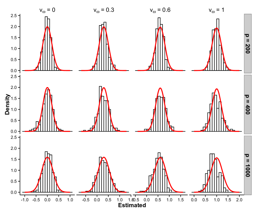
Figure 1: The histograms of the estimators for randomly selected entries with values $v_{\omega}=0,0.3,0.6$ and $1$ in three models listed in Table 1. The theoretical normal density curves are shown as solid curves. The variance for each curve is $(\omega_{ii}\omega_{jj}+\omega_{ij}^{2})/n$, the inverse of the Fisher information.

5.2 Support recovery

In this section, we evaluate the performance of the proposed ANTAC method and competing methods in support recovery with different simulation settings. ANTAC always performs among the best under all model settings. Under the Heterogeneous Model setting, the ANTAC achieves superior precision and recall rates and performs significantly better than others. Besides, ANTAC is computationally more efficient compared to a state-of-art method CAPME due to its tuning free property.

Homogeneous Model

We consider three models with corresponding $\left\{p,q,n\right\}$ listed in Table 2, which are similar to the models listed in Table 2 and used in (?). Since every model has identical values along the diagonal, we call them “Homogeneous Model”. In terms of the support recovery, ANTAC performs among the best in all three models, although the performance from all procedures is not satisfactory due to the intrinsic difficulty of support recovery problem for models considered.

We generate the $p\times q$ coefficient matrix $\Gamma$ in the same way as Section 5.1,

$$\Gamma_{ij}\overset{i.i.d.}{\sim}N\left(0,1\right)\cdot\text{Bernoulli}(0.025).$$

The off-diagonal entries of the $p\times p$ precision matrix $\Omega$ are generated as follows,

$$\omega_{ij}\overset{i.i.d.}{\sim}N\left(0,1\right)\cdot\text{Bernoulli}(\pi),$$

where the probability of being nonzero $\pi=P(\omega_{ij}\neq 0)$ is shown in Table 2 for three models respectively. We generate $50$ replicates of $X$ and $Y$ for each of the three models.

Table 2: Model parameters used in the simulation of support recovery.

	($p$, $q$, $n$)	$P(\Gamma_{ij}\neq 0)$	$\pi=P(\omega_{ij}\neq 0)$, $i\neq j$
Model 1	(200, 200, 200)	0.025	0.025
Model 2	(200, 100, 300)	0.025	0.025
Model 3	(800, 200, 200)	0.025	0.010

We compare our method with graphical Lasso (GLASSO) (?), a state-of-art method — CAPME (?) and a conditional GLASSO procedure (short as cGLASSO), where we apply the same scaled lasso procedure as the first stage of the proposed method and then estimate the precision matrix by GLASSO. This cGLASSO procedure is similar to that considered in ? except that in the first stage ? applies ordinary lasso rather than the scaled lasso, which requires another cross-validation for this step. For GLASSO, the precision matrix is estimated directly from the sample covariance matrix without taking into account the effects from $X$. The tuning parameter for the $l_{1}$ penalty is selected using five-fold cross validation by maximizing the log-likelihood function. For CAPME, the tuning parameters $\lambda_{1}$ and $\lambda_{2}$, which control the penalty in the two stages of regression, are chosen using five-fold cross validation by maximizing the log-likelihood function. The optimum is achieved via a grid search on $\{(\lambda_{1},\lambda_{2})\}$. For Models 1 and 2, $10\times 10$ grid is used and for Model 3, $5\times 5$ grid is used because of the computational burden. Specifically, we use the CAPME package implemented by the authors of (?). For Model 3, each run with $5\times 5$ grid search and five-fold cross validation takes $160$ CPU hours using one core from PowerEdge M600 nodes $2.33$ GHz and $16-48$ GB RAM, whereas ANTAC takes $46$ CPU hours. For ANTAC, the parameter $\lambda_{1}$ is set to be $B_{1}/\sqrt{n-1+B_{1}^{2}},$ where $B_{1}=q_{t}(1-\frac{1}{2}\left(s_{\max,1}/q\right)^{1+\frac{\log p}{\log q}},n-1)$, $q_{t}(\cdot,n)$ is the quantile function of $t$ distribution with degrees of freedom $n$ and $s_{\max,1}=\sqrt{n}/\log q$. The parameter $\lambda_{2}$, is set to be $B_{2}/\sqrt{n-1+B_{2}^{2}}$ where $B_{2}=q_{t}(1-\left(s_{\max,2}/p\right)^{3}/2,n-1)$. For cGLASSO, the first step is the same as ANTAC. In the second step, the precision matrix is estimated by applying GLASSO to the estimated $Z$, where the tuning parameter is selected using five-fold cross validation by maximizing the log-likelihood function.

We evaluate the performance of the estimators for support recovery problem in terms of the misspecification rate, specificity, sensitivity, precision and Matthews correlation coefficient, which are defined as,

$$\text{MISR}(\hat{\Omega},\Omega) = \frac{\text{{\small FN}}+\text{{\small FP}}}{p(p-1)}\text{, SPE}=\frac{\text{{\small TN}}}{\text{{\small TN}}+\text{{\small FP}}}\text{, SEN}=\frac{\text{{\small TP}}}{\text{{\small TP}}+\text{{\small FN}}}\text{,}$$

PRE $$= \frac{\text{{\small TP}}}{\text{{\small TP}}+\text{{\small FP}}}\text{, MCC}=\frac{\text{{\small TP}}\times\text{{\small TN}}-\text{{\small FP}}\times\text{{\small FN}}}{\left[\left(\text{{\small TP}}+\text{{\small FP}}\right)\left(\text{{\small TP}}+\text{{\small FN}}\right)\left(\text{{\small TN}}+\text{{\small FP}}\right)\left(\text{{\small TN}}+\text{{\small FN}}\right)\right]^{1/2}}\text{.}$$

Here, TP, TN, FP, FN are the numbers of true positives, true negatives, false positives and false negatives respectively. True positives are defined as the correctly identified nonzero entries of the off-diagonal entries of $\Omega$. For GLASSO and CAPME, nonzero entries of $\hat{\Omega}$ are selected as edges with no extra thresholding applied. For ANTAC, edges are selected by the theoretical bound with $\xi_{0}=2$ . The results are summarized in Table 3. It can be seen that ANTAC achieves superior specificity and precision. Besides, ANTAC has the best overall performance in terms of the Matthews correlation coefficient.

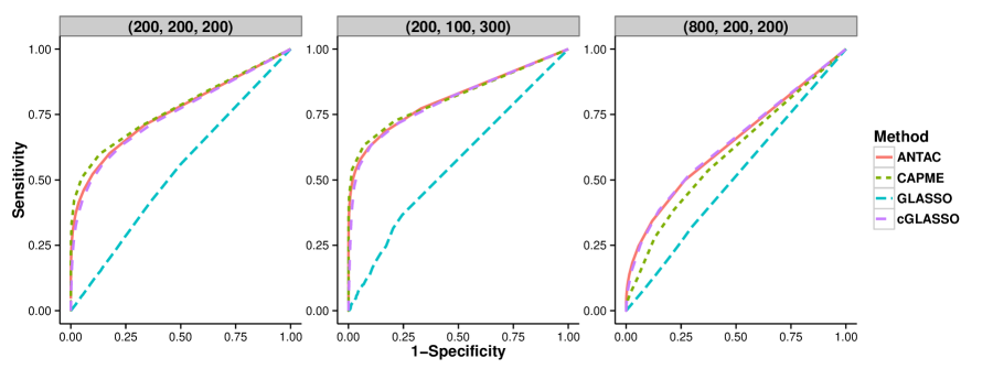
Figure 2: The ROC curves for different methods. For GLASSO or cGLASSO, the ROC curve is obtained by varying its tuning parameter. For CAPME, $\lambda_{1}$ is fixed as the value selected by the cross validation and the ROC curve is obtained by varying $\lambda_{2}$. For ANTAC, the ROC curve is obtained by varying the cut-off on P-values.

We further construct ROC curves to check how this result would vary by changing the tuning parameters. For GLASSO or cGLASSO, the ROC curve is obtained by varying the tuning parameter. For CAPME, $\lambda_{1}$ is fixed as the value selected by the cross validation and the ROC curve is obtained by varying $\lambda_{2}$. For proposed ANTAC method, the ROC curve is obtained by varying the thresholding level $\xi_{0}$. When $p$ is small, CAPME, cGLASSO and ANTAC have comparable performance. As $p$ grows, both ANTAC and cGLASSO outperform CAPME.

Table 3: Simulation results of the support recovery for homogeneous models based on 50 replications. Specifically, the performance is measured by misspecification rate, specificity, sensitivity (recall rate), precision and the Matthews correlation coefficient with all the values multiplied by 100. Numbers in parentheses are the simulation standard deviations.

	($p$, $q$, $n$)	Method	MISR	SPE	SEN	PRE	MCC
Model 1	(200, 200, 200)	GLASSO	35(1)	65(1)	37(2)	2(0)	1(1)
		cGLASSO	25(6)	76(6)	64(7)	6(1)	8(1)
		CAPME	2(0)	100(0)	4(1)	96(1)	21(1)
		ANTAC	2(0)	100(0)	4(0)	88(8)	18(2)
Model 2	(200, 100, 300)	GLASSO	43(0)	57(0)	51(2)	3(0)	3(1)
		cGLASSO	5(0)	97(0)	47(1)	25(1)	32(1)
		CAPME	4(0)	97(0)	56(1)	29(1)	39(1)
		ANTAC	2(0)	100(0)	22(1)	97(2)	46(1)
Model 3	(800, 200, 200)	GLASSO	19(1)	81(1)	19(1)	1(0)	0(0)
		cGLASSO	1(0)	100(0)	0(0)	100(0)	2(0)
		CAPME	1(0)	100(0)	0(0)	0(0)	0(0)
		ANTAC	1(0)	100(0)	7(0)	71(2)	22(1)

The purpose of simulating “Homogeneous Model” is to compare the performance of ANTAC and other procedures under models with similar settings used in ?. Overall the performance from all procedures is not satisfactory due to the difficulty of support recovery problem. All nonzero entries are sampled from a standard normal. Hence, most signals are very weak and hard to be recovered by any method, although ANTAC performs among the best in all three models.

Heterogeneous Model

We consider some models where the diagonal entries of the precision matrix have different values. These models are different from “Homogeneous Model” and we call them “Heterogeneous Model”. The performance of ANTAC and other procedures are explored under “Magnified Block” model and “Heterogeneous Product” model, respectively. The ANTAC performs significantly better than GLASSO, cGLASSO and CAMPE in both settings.

In “Magnified Block” model, we apply the following randomized procedure to choose $\Omega$ and $\Gamma$. We first simulate a $50\times 50$ matrix $\Omega_{B}$ with diagonal entries being 1 and each non-diagonal entry i.i.d. being nonzero with $P(\omega_{ij}\neq 0)=0.02$. If $\omega_{ij}\neq 0$, we sample $\omega_{ij}$ from $\{0.4,0.5\}$. Then we generate two matrices by multiplying $\Omega_{B}$ by $5$ and $10$, respectively. Then we align three matrices along the diagonal, resulting in a block diagonal matrix $\Omega$ with sequentially magnified signals. A visualization of the simulated precision matrix is shown in Figure 3. The $150\times 100$ matrix $\Gamma$ is simulated with each entry being nonzero i.i.d. follows $N(0,1)$ with $P(\Gamma_{ij}\neq 0)=0.05$. Once the matrices $\Omega$ and $\Gamma$ are chosen, $50$ replicates of $X$ and $Y$ are generated.

In “Heterogeneous Product” model, the matrices $\Omega$ and $\Gamma$ are chosen in the following randomized way. We first simulate a $200\times 200$ matrix $\Omega$ with diagonal entries being $1$ and each non-diagonal entry i.i.d. being nonzero with $P(\omega_{ij}\neq 0)=0.005$. If $\omega_{ij}\neq 0$, we sample $\omega_{ij}$ from $\{0.4,0.5\}$. Then we replace the $100\times 100$ submatrix at bottom-right corner by multiplying the $100\times 100$ submatrix at up-left corner by $2$, which results in a precision matrix with possibly many different product values $\omega_{ii}\sigma_{jj}$ over all $i,j$ pairs, where $\sigma_{jj}$ is the $j$th diagonal entry of the covariance matrix $\Sigma=\left(\sigma_{kl}\right)_{p\times p}=\Omega^{-1}$. Thus we call it “Heterogeneous Product” model. A visualization of the simulated precision matrix is shown in Figure 4. The $200\times 100$ matrix $\Gamma$ is simulated with each entry being nonzero i.i.d. follows $N(0,1)$ with $P(\Gamma_{ij}\neq 0)=0.05$. Once $\Omega$ and $\Gamma$ are chosen, $50$ replicates of $X$ and $Y$ are generated.

We compare our method with GLASSO, CAPME and cGLASSO procedures in “Heterogeneous Model”. We first compare the performance of support recovery when a single procedure from each method is applied. The tuning parameters for each procedure are set in the same way as in “Homogeneous Model” except that for CAPME, the optimal tuning parameter is achieved via a $10\times 10$ grid search on $\{(\lambda_{1},\lambda_{2})\}$ by five-fold cross validation. We summarize the support recovery results in Table 4. A visualization of the support recovery result for a replicate of “Magnified Block” model and a replicate of “Heterogeneous Product” model are shown in Figure 3 and 4 respectively. In both models, ANTAC significantly outperforms others and achieves high precision and recall rate. Specifically, ANTAC has precision of $0.99$ for two models respectively while no other procedure achieves precision rate higher than $0.21$ in either model. Besides, ANTAC returns true sparse graph structure while others report much denser results.

Table 4: Simulation results of the support recovery for heterogeneous models based on 50 replications. The performance is measured by overall error rate, specificity, sensitivity (recall rate), precision and the Matthews correlation coefficient with all the values multiplied by 100. Numbers in parentheses are the simulation standard deviations.

	($p$, $q$, $n$)	Method	MISR	SPE	SEN	PRE	MCC
Magnified Block	(150, 100, 300)	GLASSO	54(0)	46(0)	80(4)	1(0)	4(1)
		cGLASSO	14(0)	86(0)	99(1)	4(0)	19(0)
		CAPME	1(0)	99(0)	99(0)	24(2)	58(1)
		ANTAC	0(0)	100(0)	98(1)	99(1)	99(1)
Heterogeneous Product	(200, 100, 300)	GLASSO	42(0)	58(0)	85(3)	1(0)	6(0)
		cGLASSO	12(0)	88(0)	100(0)	4(0)	18(0)
		CAPME	4(0)	96(0)	97(0)	15(0)	33(0)
		ANTAC	0(0)	100(0)	80(3)	99(1)	89(2)

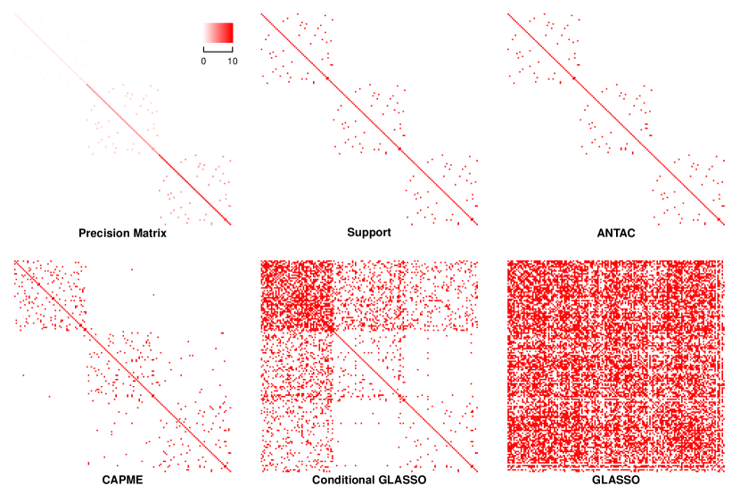
Figure 3: Heatmap of support recovery using different methods for a “Magnified Block” model.

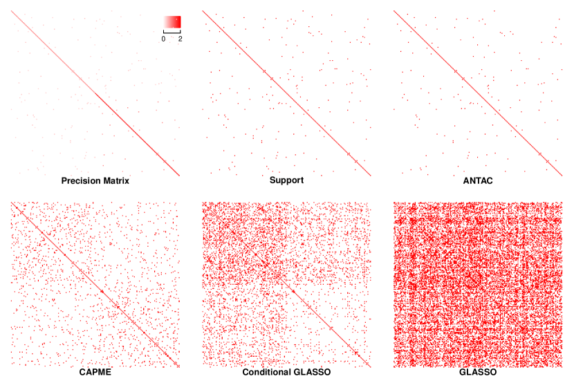
Figure 4: Heatmap of support recovery using different methods for a “Heterogeneous Product” model.

Moreover, we construct the precision-recall curve to compare a sequence of procedures from different methods. In terms of precision-recall curve, CAPME has closer performance as the proposed method in “Magnified Block” model whereas cGLASSO has closer performance as the proposed method in “Heterogeneous Product” model, which indicates the proposed method performs comparable to the better of CAPME and cGLASSO. Another implication indicates from the precision-recall curve is that while the tuning free ANTAC method is always close to the best point along the curve created by using different values of threshold $\xi_{0}$, CAPME and cGLASSO via cross validation cannot select the optimal parameters on their corresponding precision-recall curves, even though one of them has potentially good performance when using appropriate tuning parameters. Here is an explanation why the ANTAC procedure is better than CAPME and cGLASSO in “Magnified Block” model and “Heterogeneous Product” model settings. Recall that in the second stage, CAPME applies the same penalty level $\lambda$ for each entry of the difference $\Omega\hat{\Sigma}-I$, where $\hat{\Sigma}$ denotes the sample covariance matrix, but the $i,j$ entry has variance $\omega_{ii}\sigma_{jj}$ after scaling. Thus CAPME may not recover the support well in the “Heterogeneous Product” model settings, where the variances of different entries may be very different. As for the cGLASSO, we notice that essentially the same level of penalty is put on each entry $\omega_{ij}$ while the variance of each entry in the $i$th row $\Omega_{i\cdot}$ depends on $\omega_{ii}$. Hence we cannot expect cGLASSO performs very well in the “Magnified Block” model settings, where the diagonals $\omega_{ii}$ vary a lot. In contrast, the ANTAC method adaptively puts the right penalty level (asymptotic variance) for each estimate of $\omega_{ij}$, therefore it works well in either setting.

Figure 5: The precision-recall curves for “Magnified Block” model and “Heterogeneous Product” model using different methods. For GLASSO or cGLASSO, the curve is obtained by varying its tuning parameter. For CAPME, $\lambda_{1}$ is fixed as the value selected by the cross validation and the curve is obtained by varying $\lambda_{2}$. For ANTAC, the precision-recall curve is obtained by varying threshold level $\xi_{0}$. The points on the curves correspond to the results obtained by cross-validation for GLASS, cGLASS and CAPME and by using theoretical threshold level $\xi_{0}=2$ for tuning free ANTAC.

Overall, the simulation results on heterogeneous models reveal the appealing practical properties of the ANTAC procedure. Our procedure enjoys tuning free property and has superior performance. In contrast, it achieves better precision and recall rate than the results from CAPME and cGLASSO using cross validation. Although in terms of precision-recall curve, the better of CAPME and cGLASSO is comparable with our procedure, generally the optimal sensitivity and specificity could not be obtained through cross-validation.

6 Application to an eQTL study

We apply the ANTAC procedure to a yeast dataset from ? (GEO accession number GSE9376), which consists of 5,493 gene expression probes and 2,956 genotyped markers measured in 109 segregants derived from a cross between BY and RM treated with glucose. We find the proposed method achieves both better interpretability and accuracy in this example.

There are many mechanisms leading to the dependency of genes at the expression level. Among those, the dependency between transcription factors (TFs) and their regulated genes has been intensively investigated. Thus the gene-TF binding information could be utilized as an external biological evidence to validate and interpret the estimation results. Specifically, we used the high-confidence TF binding site (TFBS) profiles from m:Explorer, a database recently compiled using perturbation microarray data, TF-DNA binding profiles and nucleosome positioning measurements (?).

We first focus our analysis on a medium size dataset that consists of 121 genes on the yeast cell cycle signaling pathway (from the Kyoto Encyclopedia of Genes and Genomes database (?)). There are 119 markers marginally associated with at least 3 of those 121 genes with a Bonferroni corrected P-value less than 0.01. The parameters $\lambda_{1}$ and $\lambda_{2}$ for the ANTAC method are set as described in Theorem 3. 55 edges are identified using a cutoff of 0.01 on the FDR controlled P-values and 200 edges with a cutoff of 0.05. The number of edges goes to 375 using a cutoff of 0.1. For the purpose of visualization and interpretation, we further focus on 55 edges resulted from the cutoff of 0.01.

We then check how many of these edges involve at least one TF and how many TF-gene pairs are documented in the m:Explorer database. In 55 detected edges, 12 edges involve at least one TF and 2 edges are documented. In addition, we obtain the estimation of precision matrix from CAPME, where the tuning parameters $\lambda_{1}=0.356$ and $\lambda_{2}=0.5$ are chosen by five-fold cross validation. To compare with the results from ANTAC, we select top 55 edges from CAPME solution based on the magnitude of partial correlation. Within these 55 edges, 13 edges involve at least one TF and 2 edges are documented. As shown in Figure 6, 22 edges are detected by both methods. Our method identifies a promising cell cycle related subnetwork featured by CDC14, PDS1, ESP1 and DUN1, connecting through GIN4, CLB3 and MPS1. In the budding yeast, CDC14 is a phosphatase functions essentially in late mitosis. It enables cells to exit mitosis through dephosphorylation and activation of the enemies of CDKs (?). Throughout G1, S/G2 and early mitosis, CDC14 is inactive. The inactivation is partially achieved by PDS1 via its inhibition on an activator ESP1 (?). Moreover, DUN1 is required for the nucleolar localization of CDC14 in DNA damage-arrested yeast cells (?).

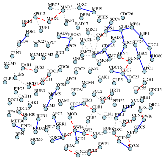
Figure 6: Visualization of the network constructed from yeast cell cycle expression data by CAPME and the proposed ANTAC method. For ANTAC, 55 edges are identified using a cutoff of 0.01 on the FDR controlled p-values. For CAPME, top 55 edges are selected based on the magnitude of partial correlation. 22 common edges detected by both methods are shown in dashed lines. Edges only detected by the proposed method are shown in solid lines. CAPME-specific edges are shown in dotted lines.

We then extend the analysis to a larger dataset constructed from GSE9376. For 285 TFs documented in m:Explorer database, expression levels of 20 TFs are measured in GSE9376 with variances greater than 0.25. For these 20 TFs, 875 TF-gene interactions with 377 genes with variances greater than 0.25 are documented in m:Explorer. Applying the screening strategy as the previous example, we select 644 genetic markers marginally associated with at least 5 of the 377 genes with a Bonferroni corrected P-value less than 0.01. We apply the proposed ANTAC method and CAPME to this new dataset. For ANTAC, the parameters $\lambda_{1}$ and $\lambda_{2}$ are set as described in Theorem 3. For CAPME, the tuning parameters $\lambda_{1}=0.089$ and $\lambda_{2}=0.281$ are chosen by five-fold cross validation. We use TF-gene interactions documented in m:Explorer as an external biological evidence to validate the results. The results are summarized in Table 5. For ANTAC, 540 edges are identified using a cutoff of 0.05 on the FDR controlled P-values. Within these edges, 67 edges are TF-gene interactions and 44 out of 67 are documented in m:Explorer. In comparison, 8499 nonzero edges are detected by CAPME, where 915 edges are TF-gene interactions and 503 out of 915 are documented. This result is hard to interpret biologically. We further ask if identifying the same number of TF-gene interactions, which method achieves higher accuracy according to the concordance with m:Explorer. Based on the magnitude of partial correlation, we select top 771 edges from the CAPME solution, which capture 67 TF-gene interactions. Within these interactions, 38 are documented in m:Explorer. Thus in this example, the proposed ANTAC method achieves both better interpretability and accuracy.

Table 5: Results for a dataset consists of 644 markers and 377 genes, which was constructed from GSE9376.

Method	Solution	Total $\#$ of gene-gene	$\#$ of TF-gene	$\#$ of TF-gene	Documented
	Criteria	interactions	interactions	interactions documented	Proportion
ANTAC	FDR controlled P-values $\leq$0.05	540	67	44	65%
CAPME	Magnitude of partial correlation	771	67	38	57%
CAPME	Nonzero entries	8499	915	503	55%

7 Proof of Main Theorems

In this section, we will prove the main results Theorems 1 and 2.

7.1 Proof of Theorem 1

This proof is based on the key lemma, Lemma 5, which is deterministic in nature. We apply Lemma 5 with $\mathbf{R=D}b^{true}+\mathbf{E}$ replaced by $\mathbf{Y}_{j}\mathbf{=X}\gamma_{j}+\mathbf{Z}_{j},$ $\lambda$ replaced by $\lambda_{1}$ and sparsity $s$ replaced by $s_{1}$. The following lemma is the key to the proof.

Lemma 1

There exist some constants $C_{k}^{\prime}$, $1\leq k\leq 3$ such that for each $1\leq j\leq p$,

$$\left\|\mathbf{\gamma}_{j}-\mathbf{\hat{\gamma}}_{j}\right\|_{1} \leq C_{1}^{\prime}\lambda_{1}s_{1}\text{,}$$ (33)

$$\left\|\mathbf{\gamma}_{j}-\mathbf{\hat{\gamma}}_{j}\right\| \leq C_{2}^{\prime}\lambda_{1}\sqrt{s_{1}}\text{,}$$ (34)

$$\left\|\mathbf{X}\left(\mathbf{\gamma}_{j}-\mathbf{\hat{\gamma}}_{j}\right)\right\|^{2}/n \leq C_{3}^{\prime}\lambda_{1}^{2}s_{1}\text{,}$$ (35)

with probability $1-o\left(q^{-\delta_{1}+1}\right)$.

With the help of the lemma above, it’s trivial to finish our proof. In fact, $\left\|\mathbf{\hat{Z}}_{j}-\mathbf{Z}_{j}\right\|^{2}=\left\|\mathbf{X}\left(\mathbf{\gamma}_{j}-\mathbf{\hat{\gamma}}_{j}\right)\right\|^{2}$ and hence Equation (14) immediately follows from result (35). Equations (15) and (16) are obtained by the union bound and Equations (33) and (34) because of the following relationship,

$$\left\|\mathbf{\hat{\Gamma}}-\mathbf{\Gamma}\right\|_{l_{\infty}} = \max_{j}\left\|\mathbf{\gamma}_{j}-\mathbf{\hat{\gamma}}_{j}\right\|_{1}\text{,}$$

$$\frac{1}{p}\left\|\mathbf{\hat{\Gamma}}-\mathbf{\Gamma}\right\|_{F}^{2} = \frac{1}{p}\sum_{j=1}^{p}\left\|\mathbf{\gamma}_{j}-\mathbf{\hat{\gamma}}_{j}\right\|^{2}\text{.}$$

It is then enough to prove Lemma 1 to complete the proof of Theorem 1.

Proof of Lemma 1

The Lemma is an immediate consequence of Lemma 5 applied to $\mathbf{Y}_{j}\mathbf{=X}\gamma_{j}+\mathbf{Z}_{j}$ with tuning parameter $\lambda_{1}$ and sparsity $s_{1}$. To show the union of Equations (33)-(35) holds with high probability $1-o\left(q^{-\delta_{1}+1}\right)$, we only need to check the following conditions of the Lemma 5 hold with probability at least $1-o\left(q^{-\delta_{1}+1}\right)$,

$$I_{1} = \left\{\nu\leq\theta^{ora}\lambda_{1}\frac{\xi-1}{\xi+1}\left(1-\tau\right)\text{ for some }\xi>1\right\}\text{,}$$

$$I_{2} = \left\{\frac{\left\|\mathbf{X}_{k}\right\|}{\sqrt{n}}\in\left[1/A_{1},A_{1}\right]\text{ for all }k\right\}\text{,}$$

$$I_{3} = \left\{\theta^{ora}\in\left[1/A_{2},A_{2}\right]\text{, where }\theta^{ora}=\frac{\left\|\mathbf{Z}_{j}\right\|}{\sqrt{n}}\text{.}\right\}\text{,}$$

$$I_{4} = \left\{\begin{array}[]{c}\frac{\mathbf{W}^{T}\mathbf{W}}{n}\text{ satisfies lower-RE with }\left(\alpha_{1},\zeta\left(n,q\right)\right)\text{ s.t.}\\ s_{1}\zeta\left(n,q\right)8\left(1+\xi\right)^{2}A_{1}^{2}\leq\min\{\frac{\alpha_{1}}{2},1\}\end{array}\right\}\text{,}$$

where we set $\xi=3/\varepsilon_{1}+1$ for the current setting, $A_{1}=C_{A_{1}}\max\left\{B,\sqrt{M_{1}}\right\}$ under Condition $3$ and $A_{1}=C_{A_{1}}\sqrt{M_{1}}$ under Condition $3^{\prime}$ for some universal constant $C_{A_{1}}>0$, $A_{2}=\sqrt{2M_{2}}$, $\alpha_{1}=\frac{1}{2M_{1}}$ and $\zeta\left(n,q\right)=o(1/s_{1})$. Let us still define $\mathbf{W=X}\cdot diag\left(\frac{\sqrt{n}}{\left\|\mathbf{X}_{k}\right\|}\right)$ as the standardized $\mathbf{X}$ in Lemma 5 of Section 8.

We will show that

$$\mathbb{P}\left\{I_{1}^{c}\right\} \leq O\left(q^{-\delta_{1}+1}/\sqrt{\log q}\right)\text{,}$$

$$\mathbb{P}\left\{I_{i}^{c}\right\} \leq o(q^{-\delta_{1}})\text{ for }i=2,3\text{ and }4\text{,}$$

which implies

$$\mathbb{P}\left\{E_{j}\right\}\geq 1-o\left(q^{-\delta_{1}+1}\right)\text{,}$$

where $E_{j}$ is the union of $I_{1}$ to $I_{4}$. We will first consider $\mathbb{P}\left\{I_{2}^{c}\right\}$ and $\mathbb{P}\left\{I_{3}^{c}\right\}$, then $\mathbb{P}\left\{I_{4}^{c}\right\}$, and leave $\mathbb{P}\left\{I_{1}^{c}\right\}$ to the last, which relies on the bounds for $\mathbb{P}\left\{I_{i}^{c}\right\}$, $2\leq i\leq 4$.

(1). To study $\mathbb{P}\left\{I_{2}^{c}\right\}$ and $\mathbb{P}\left\{I_{3}^{c}\right\}$, we need the following Bernstein-type inequality (See e.g. (?), Section $5.2.4$ for the inequality and definitions of norms $\left\|\cdot\right\|_{\varphi_{2}}$ and $\left\|\cdot\right\|_{\varphi_{1}}$) to control the tail bound for sum of i.i.d. sub-exponential variables,

$$\mathbb{P}\left\{\left|\sum_{i=1}^{n}U_{i}\right|\geq tn\right\}\leq 2\exp\left(-cn\min\left\{\frac{t^{2}}{K^{2}},\frac{t}{K}\right\}\right)\text{,}$$ (37)

for $t>0$, where $U_{i}$ are i.i.d. centered sub-exponential variables with parameter $\left\|U_{i}\right\|_{\varphi_{1}}\leq K$ and $c$ is some universal constant. Notice that $\theta^{ora}=\left\|\mathbf{Z}_{j}\right\|/\sqrt{n}$ with $\mathbf{Z}_{j}^{(1)}\sim N\left(0,\sigma_{jj}\right)$, and $\mathbf{X}_{k}^{(1)}$ is sub-gaussian with parameter $\left\|\mathbf{X}_{k}^{(1)}\right\|_{\varphi_{2}}\in\left[c_{\varphi 2}M_{1}^{-1/2},C_{\varphi 2}B\right]$ by Conditions $2$ and $3$ with some universal constants $c_{\varphi 2}$ and $C_{\varphi 2}$ (all formulas involving $\varphi_{1}$ or $\varphi_{2}$ parameter of $\mathbf{X}_{k}^{(1)}$ replace “$B$” by “$\sqrt{M_{1}}$” under Condition $3^{\prime}$ hereafter). The fact that sub-exponential is sub-gaussian squared implies that there exists some universal constant $C_{1}>0$ such that

$$n\left(\left(\theta^{ora}\right)^{2}-\sigma_{jj}\right)\text{ is sum of i.i.d. sub-exponential with }\varphi_{1}\text{ parameter }C_{1}\sigma_{jj}\text{,}$$

$$\left\|\mathbf{X}_{k}\right\|^{2}-n\mathbb{E}x_{k}^{2}\text{ is sum of i.i.d. sub-exponential with }\varphi_{1}\text{\ parameter }\left\|\left(\mathbf{X}_{k}^{(1)}\right)^{2}\right\|_{\varphi_{1}}\text{.}$$

Note that $\sigma_{jj}\in\left[1/M_{2},M_{2}\right]$ by Condition $2$ and $\left\|\left(\mathbf{X}_{k}^{(1)}\right)^{2}\right\|_{\varphi_{1}}\in\left[c_{\varphi 1}^{\prime}M_{1}^{-1},C_{\varphi 1}^{\prime}B^{2}\right]$ with some universal constants $c_{\varphi 1}^{\prime}$ and $C_{\varphi 1}^{\prime}$. Let $A_{1}=C_{A_{1}}\max\left\{B,\sqrt{M_{1}}\right\}$ and $A_{2}=\sqrt{2M_{2}}$ for some large constant $C_{A_{1}}$. Equation (37) with a sufficiently small constant $c_{0}$ implies

$$\mathbb{P}\left\{I_{3}^{c}\right\} = \mathbb{P}\left\{\left(\theta^{ora}\right)^{2}\notin\left[1/A_{2}^{2},A_{2}^{2}\right]\right\}\leq\mathbb{P}\left\{n\left|\left(\theta^{ora}\right)^{2}-\sigma_{jj}\right|\geq\frac{\sigma_{jj}}{2}n\right\}$$ (38)

$$\leq 2\exp\left(-C^{{}^{\prime}}n\right)\leq o(q^{-\delta_{1}})\text{,}$$

and

$$\mathbb{P}\left\{I_{2}^{c}\right\} = \mathbb{P}\left\{\frac{\left\|\mathbf{X}_{k}\right\|^{2}}{n}\notin\left[1/A_{1}^{2},A_{1}^{2}\right]\text{ for some }k\right\}$$ (39)

$$\leq q\mathbb{P}\left\{\left|\left\|\mathbf{X}_{k}\right\|^{2}-n\mathbb{E}x_{k}^{2}\right|>c_{0}\left\|\left(\mathbf{X}_{k}^{(1)}\right)^{2}\right\|_{\varphi_{1}}n\right\}\leq q2\exp\left(-C^{\prime}n\right)\leq o(q^{-\delta_{1}})\text{.}$$

(2). To study the lower-RE condition of $\frac{\mathbf{W}^{T}\mathbf{W}}{n}$, we essentially need to study $\frac{\mathbf{X}^{T}\mathbf{X}}{n}$. On the event $I_{2}$, it’s easy to see that if $\frac{\mathbf{X}^{T}\mathbf{X}}{n}$ satisfies lower-RE with $\left(\alpha_{x},\zeta_{x}\left(n,q\right)\right)$, then $\frac{\mathbf{W}^{T}\mathbf{W}}{n}$ satisfies lower-RE with $\left(\alpha_{1},\zeta\right)=\left(\alpha_{x}A_{1}^{-2},\zeta_{x}A_{1}^{2}\right)$, since $\mathbf{W}=\mathbf{X}diag\left(\frac{\sqrt{n}}{\left\|X_{k}\right\|}\right)$ and $\frac{\left\|\mathbf{X}_{k}\right\|}{\sqrt{n}}\in\left[1/A_{1},A_{1}\right]$ on event $I_{2}$. Moreover, to study the lower-RE condition, the following lemma implies that we only need to consider the behavior of $\frac{\mathbf{X}^{T}\mathbf{X}}{n}$ on sparse vectors.

Lemma 2

For any symmetric matrix $\Delta_{q\times q}$, suppose $\left|v^{T}\Delta v\right|\leq\delta$ for any unit $2s$ sparse vector $v\in\mathbb{R}^{q}$, i.e. $\left\|v\right\|=1$ and $v\in\mathbb{B}_{0}\left(2s\right)=\left\{a:\sum_{i=1}^{q}1\left\{a_{i}\neq 0\right\}\leq 2s\right\}$, then we have

$$\left|v^{T}\Delta v\right|\leq 27\delta\left(\left\|v\right\|^{2}+\frac{1}{s}\left\|v\right\|_{1}^{2}\right)\text{ for any }v\in\mathbb{R}^{q}\text{.}$$

See Supplementary Lemma $12$ in (?) for the proof. With a slight abuse of notation, we define $\Sigma_{x}=Cov\left(X^{\left(1\right)}\right)$. By applying Lemma 2 on $\frac{\mathbf{X}^{T}\mathbf{X}}{n}-\Sigma_{x}$ and Condition $2$, $v^{T}\Sigma_{x}v\geq$ $\frac{1}{M_{1}}\left\|v\right\|^{2}$, we know that $\frac{\mathbf{X}^{T}\mathbf{X}}{n}$ satisfies lower-RE $\left(\alpha_{x},\zeta_{x}\left(n,q\right)\right)$ with

$$\alpha_{x}\geq\frac{1}{M_{1}}\left(1-\frac{27}{L}\right)\text{ and }\zeta_{x}\left(n,q\right)\leq\frac{27}{s_{1}M_{1}L}\text{,}$$ (40)

provided

$$\left|v^{T}\left(\frac{\mathbf{X}^{T}\mathbf{X}}{n}-\Sigma_{x}\right)v\right|\leq\frac{1}{LM_{1}}\text{ for all }v\in\mathbb{B}_{0}\left(2s_{1}\right)\text{ with }\left\|v\right\|=1\text{,}$$ (41)

which implies that the population covariance matrix $\Sigma_{x}$ and its sample version $\frac{\mathbf{X}^{T}\mathbf{X}}{n}$ behave similarly on all $2s_{1}$ sparse vectors.

Now we show Equation (41) holds under Conditions $3$ and $3^{\prime}$ respectively for a sufficiently large constant $L$ such that the inequality in the event $I_{4}$ holds. Under Condition $3^{\prime}$, $X^{\left(1\right)}$ is jointly sub-gaussian with parameter $\left(M_{1}\right)^{1/2}$. A routine one-step chaining (or $\delta$-net) argument implies that there exists some constant $c_{sg}>0$ such that

$$\mathbb{P}\left\{\sup_{v\in\mathbb{B}_{0}\left(2s_{1}\right)}\left|v^{T}\left(\frac{\mathbf{X}^{T}\mathbf{X}}{n}-\Sigma_{x}\right)v\right|>t\left\|v\right\|^{2}\right\}\leq 2\exp\left(-c_{sg}n\min\left\{\frac{t^{2}}{M_{1}^{2}},\frac{t}{M_{1}}\right\}+2s_{1}\log q\right)\text{.}$$ (42)

See e.g. Supplementary Lemma $15$ in (?) for the proof. Hence by picking small $t=\frac{1}{LM_{1}}$ with any fixed but arbitrary large $L,$ the sparsity condition (17) $s_{1}=o\left(\frac{n}{\log q}\right)$ and Equation (42) imply that Equation (41) holds with probability $1-$ $o\left(p^{-\delta_{1}}\right)$.

Under Condition $3$, if $s_{1}=o\left(\sqrt{\frac{n}{\log q}}\right)$, Hoeffding’s inequality and a union bound imply that

$$\mathbb{P}\left\{\left\|\frac{\mathbf{X}^{T}\mathbf{X}}{n}-\Sigma_{x}\right\|_{\infty}>2B\sqrt{\frac{(1+\delta_{1})\log q}{n}}\right\}\leq 2q^{-2\delta_{1}}\text{,}$$

where the norm $\left\|\cdot\right\|_{\infty}$ denotes the entry-wise supnorm and $\left\|X^{\left(1\right)}\right\|_{\infty}\leq B$ (see, e.g. (?) Proposition $2.7$). Thus with probability $1-$ $o\left(q^{-\delta_{1}}\right)$, we have for any $v\in\mathbb{B}_{0}\left(2s_{1}\right)$ with $\left\|v\right\|=1$,

$$\left|v^{T}\left(\frac{\mathbf{X}^{T}\mathbf{X}}{n}-\Sigma_{x}\right)v\right|\leq\left\|\frac{\mathbf{X}^{T}\mathbf{X}}{n}-\Sigma_{x}\right\|_{\infty}\left\|v\right\|_{1}^{2}\leq 2B\sqrt{\frac{(1+\delta_{1})\log q}{n}}\frac{1}{2s_{1}}=o(1)\text{,}$$

where the last inequality follows from $\left\|v\right\|_{1}\leq\sqrt{2s_{1}}\left\|v\right\|$ for any $v\in\mathbb{B}_{0}\left(2s_{1}\right)$. Therefore we have Equation (41) holds with probability $1-$ $o\left(q^{-\delta_{1}}\right)$ for any arbitrary large $L$. If $s_{1}=o\left(\frac{n}{\log^{3}n\log q}\right)$, an involved argument using Dudley’s entropy integral and Talagrand’s concentration theorem for empirical processes implies (see, (?) Theorem $23$ and its proof) Equation (41) holds with probability $1-$ $o\left(q^{-\delta_{1}}\right)$ for any fixed but arbitrary large $L$.

Therefore we showed that under Condition $3$ or $3^{\prime}$, Equation (41) holds with probability $1-$ $o\left(q^{-\delta_{1}}\right)$ for any arbitrary large $L.$ Consequently, Equation (40) with $\left(\alpha_{1},\zeta\right)=\left(\alpha_{x}A_{1}^{-2},\zeta_{x}A_{1}^{2}\right)$ on event $I_{2}$ implies that we can pick $\alpha_{1}=\frac{1}{2M_{1}}$ and sufficiently small $\zeta$ such that event $I_{4}$ holds with probability $1-$ $o\left(q^{-\delta_{1}}\right)$.

(3). Finally we study the probability of event $I_{1}$. The following tail probability of $t$ distribution is helpful in the analysis.

Proposition 1

Let $T_{n}$ follows a $t$ distribution with $n$ degrees of freedom. Then there exists $\epsilon_{n}\rightarrow 0$ as $n\rightarrow\infty$ such that $\forall t>0$

$$\mathbb{P}\left\{T_{n}^{2}>n\left(e^{2t^{2}/(n-1)}-1\right)\right\}\leq\left(1+\epsilon_{n}\right)e^{-t^{2}}/\left(\pi^{1/2}t\right)\text{.}$$

Please refer to (?) Lemma 1 for the proof. Recall that $I_{1}=\left\{\frac{\nu}{\theta^{ora}}\leq\lambda_{1}\frac{\xi-1}{\xi+1}\left(1-\tau\right)\right\}$, where $\tau$ defined in Equation (69) satisfies that $\tau=O\left(s_{1}\lambda_{1}^{2}\right)=o\left(1\right)$ on $\cap_{i=2}^{4}I_{i}$. From the definition of $\nu$ in Equation (68) we have

$$\frac{\nu}{\theta^{ora}}=\max_{k}\left|h_{k}\right|\text{, with }h_{k}=\frac{\mathbf{W}_{k}^{T}\mathbf{Z}_{j}}{n\theta^{ora}}\text{,}$$

where each column of $\mathbf{W}$ has norm $\left\|\mathbf{W}_{k}\right\|=\sqrt{n}$. Given $\mathbf{X}$, equivalently $\mathbf{W}$, it’s not hard to check that we have $\frac{\sqrt{n-1}h_{k}}{\sqrt{1-h_{k}^{2}}}\sim t_{\left(n-1\right)}$ by the normality of $\mathbf{Z}_{j}$, where $t_{\left(n-1\right)}$ is the $t$ distribution with $\left(n-1\right)$ degrees of freedom. From Proposition 1 we have

$$\mathbb{P}\left\{\left|h_{k}\right|>\sqrt{\frac{2t^{2}}{n}}\right\}$$

$$= \mathbb{P}\left\{\frac{\left(n-1\right)h_{k}^{2}}{1-h_{k}^{2}}>\frac{2\left(n-1\right)t^{2}/n}{1-2t^{2}/n}\right\}\leq\mathbb{P}\left\{\frac{\left(n-1\right)h_{k}^{2}}{1-h_{k}^{2}}>\frac{2\left(n-1\right)t^{2}/\left(n-2\right)}{1-t^{2}/\left(n-2\right)}\right\}$$

$$\leq \mathbb{P}\left\{\frac{\left(n-1\right)h_{k}^{2}}{1-h_{k}^{2}}>\left(n-1\right)\left(e^{2t^{2}/(n-2)}-1\right)\right\}\leq\left(1+\epsilon_{n-1}\right)e^{-t^{2}}/\left(\pi^{1/2}t\right)\text{,}$$

where the first inequality holds when $t^{2}\geq 2$, and the second inequality follows from the fact $e^{x}-1\leq x/(1-\frac{x}{2})$ for $0<x<2$. Now let $t^{2}=\delta_{1}\log q>2$, and $\lambda_{1}=\left(1+\varepsilon_{1}\right)\sqrt{\frac{2\delta_{1}\log q}{n}}$ with $\xi=3/\varepsilon_{1}+1$, then we have $\lambda_{1}\frac{\xi-1}{\xi+1}\left(1-\tau\right)>\sqrt{\frac{2\delta_{1}\log q}{n}}\$and

$$\mathbb{P}\left\{\cap_{i=1}^{4}I_{i}\right\} \geq \mathbb{P}\left\{\frac{\nu}{\theta^{ora}}\leq\sqrt{\frac{2\delta_{1}\log q}{n}}\right\}-\mathbb{P}\left\{\left(\cap_{i=2}^{4}I_{i}\right)^{c}\right\}$$

$$\geq 1-q\cdot\mathbb{P}\left\{\left|h_{k}\right|>\sqrt{\frac{2\delta_{1}\log q}{n}}\right\}-\mathbb{P}\left\{\left(\cap_{i=2}^{4}I_{i}\right)^{c}\right\}$$

$$\geq 1-\left(\frac{1}{\sqrt{\pi\delta_{1}}}+o\left(1\right)\right)\frac{q^{-\delta_{1}+1}}{\sqrt{\log q}}\text{,}$$

which immediately implies $\mathbb{P}\left\{I_{1}^{c}\right\}\leq O\left(q^{-\delta_{1}+1}/\sqrt{\log q}\right)$.

7.2 Proof of Theorem 2

The whole proof is based on the results in Theorem 1. In particular with probability $1-o\left(p\cdot q^{-\delta_{1}+1}\right)$, the following events hold,

$$\frac{1}{n}\left\|\mathbf{\hat{Z}}_{j}-\mathbf{Z}_{j}\right\|^{2} \leq C_{1}s_{1}\frac{\log q}{n}\text{ for all }j\text{,}$$ (43)

$$\left\|\mathbf{\hat{\gamma}}_{j}-\mathbf{\gamma}_{j}\right\|_{1} \leq C_{2}s_{1}\sqrt{\frac{\log q}{n}}\text{ for all }j\text{.}$$ (44)

From now on the analysis is conditioned on the two events above. This proof is also based on the key lemma, Lemma 5. We apply Lemma 5 with $\mathbf{R=D}b^{true}+\mathbf{E}$ replaced by $\mathbf{\hat{Z}}_{m}\mathbf{=\hat{Z}}_{A^{c}}\beta_{m}+\mathbf{E}_{m}$ for each $m\in A=\left\{i,j\right\}$, $\lambda$ replaced by $\lambda_{2}$ and sparsity $s$ replaced by $C_{\beta}s_{2},$ where $\mathbf{E}_{m}$ is defined by the regression model Equation (7) as

$$\mathbf{E}_{m} \equiv \mathbf{\epsilon}_{m}+\Delta_{Z_{m}}$$

$$= \mathbf{\epsilon}_{m}+\left(\mathbf{\hat{Z}}_{m}-\mathbf{Z}_{m}\right)+\left(\mathbf{Z}_{A^{c}}-\mathbf{\hat{Z}}_{A^{c}}\right)\beta_{m}\text{,}$$

and $C_{\beta}=2M_{2}$ because the definition of $\beta_{m}$ in Equation (6) implies it is a weighted sum of two columns of $\Omega$ with weight bounded by $M_{2}$.

To obtain our desired result $\left|\hat{\psi}_{kl}-\psi_{kl}^{ora}\right|=\left|\mathbf{\epsilon}_{k}^{T}\mathbf{\epsilon}_{l}/n-\mathbf{\hat{\epsilon}}_{k}^{T}\mathbf{\hat{\epsilon}}_{l}/n\right|$ for each pair $k,l\in$ $A=\left\{i,j\right\}$, it’s sufficient for us to bound $\left|\mathbf{\hat{\epsilon}}_{k}^{T}\mathbf{\hat{\epsilon}}_{l}/n-\mathbf{E}_{k}^{T}\mathbf{E}_{l}/n\right|$ and $\left|\mathbf{\epsilon}_{k}^{T}\mathbf{\epsilon}_{l}/n-\mathbf{E}_{k}^{T}\mathbf{E}_{l}/n\right|$ separately and then to apply the triangle inequality. The following two lemmas are useful to establish those two bounds.

Lemma 3

There exists some constant $C_{in}>0$ such that $\left|\mathbf{\epsilon}_{k}^{T}\mathbf{\epsilon}_{l}/n-\mathbf{E}_{k}^{T}\mathbf{E}_{l}/n\right|\leq C_{in}\lambda_{1}^{2}s_{1}$ with probability $1-o\left(q^{-\delta_{1}}\right)$.

Lemma 4

There exist some constants $C_{k}^{\prime}$, $1\leq k\leq 3$ such that for each $m\in A=\left\{i,j\right\}$,

$$\left\|\beta_{m}-\hat{\beta}_{m}\right\|_{1} \leq C_{1}^{\prime}\lambda_{2}s_{2}\text{,}$$

$$\left\|\mathbf{\hat{Z}}_{A^{c}}\left(\beta_{m}-\hat{\beta}_{m}\right)\right\|^{2}/n \leq C_{2}^{\prime}\lambda_{2}^{2}s_{2}\text{,}$$

$$\left\|\mathbf{\hat{Z}}_{A^{c}}^{T}\mathbf{E}_{m}/n\right\|_{\infty} \leq C_{3}^{\prime}\lambda_{2}\text{,}$$

with probability $1-o\left(p^{-\delta_{2}+1}\right)$.

Before moving on, we point out a fact we will use several times in the proof,

$$\left\|\beta_{m}\right\|_{1}\leq 2M_{2}^{2}\text{,}$$ (46)

which follows from Equation (6) and Condition $5$. Hence we have

$$\left\|\Delta_{Z_{m}}\right\|/\sqrt{n}\leq\frac{\left\|\mathbf{\hat{Z}}_{m}-\mathbf{Z}_{m}\right\|}{\sqrt{n}}+\frac{\max_{k}\left\|\mathbf{\hat{Z}}_{k}-\mathbf{Z}_{k}\right\|}{\sqrt{n}}\left\|\beta_{m}\right\|_{1}\leq\sqrt{C_{3}s_{1}\lambda_{1}^{2}}\text{,}$$ (47)

for some constant $C_{3}>0$.

To bound the term $\left|\mathbf{\hat{\epsilon}}_{k}^{T}\mathbf{\hat{\epsilon}}_{l}/n-\mathbf{E}_{k}^{T}\mathbf{E}_{l}/n\right|$, we note that for any $k,l\in$ $A=\left\{i,j\right\}$,

$$\left|\mathbf{\hat{\epsilon}}_{k}^{T}\mathbf{\hat{\epsilon}}_{l}/n-\mathbf{E}_{k}^{T}\mathbf{E}_{l}/n\right| = \left|\left(\mathbf{E}_{k}+\mathbf{\hat{Z}}_{A^{c}}\left(\beta_{k}-\hat{\beta}_{k}\right)\right)^{T}\left(\mathbf{E}_{l}+\mathbf{\hat{Z}}_{A^{c}}\left(\beta_{l}-\hat{\beta}_{l}\right)\right)/n-\mathbf{E}_{k}^{T}\mathbf{E}_{l}/n\right|$$ (48)

$$\leq \left\|\mathbf{\hat{Z}}_{A^{c}}^{T}\mathbf{E}_{k}/n\right\|_{\infty}\left\|\beta_{k}-\hat{\beta}_{k}\right\|_{1}+\left\|\mathbf{\hat{Z}}_{A^{c}}^{T}\mathbf{E}_{l}/n\right\|_{\infty}\left\|\beta_{l}-\hat{\beta}_{l}\right\|_{1}$$

$$+\left\|\mathbf{\hat{Z}}_{A^{c}}\left(\beta_{k}-\hat{\beta}_{k}\right)\right\|\cdot\left\|\mathbf{\hat{Z}}_{A^{c}}\left(\beta_{l}-\hat{\beta}_{l}\right)\right\|/n$$

$$\leq \left(2C_{1}^{\prime}C_{3}^{\prime}+C_{2}^{\prime}\right)\lambda_{2}^{2}s_{2}\text{,}$$

where we applied Lemma 4 in the last inequality.

Lemma 3, together with Equation (48), immediately implies the desired result (23),

$$\left|\hat{\psi}_{kl}-\psi_{kl}^{ora}\right|\leq C_{4}^{\prime}\left(s_{2}\frac{\log p}{n}+s_{1}\frac{\log q}{n}\right)\text{,}$$

for some constant $C_{4}^{\prime}$ with probability $1-o\left(p\cdot q^{-\delta_{1}+1}+p^{-\delta_{2}+1}\right)$. Since the spectrum of $\Psi_{A,A}$ is bounded below by $M_{2}^{-1}$ and above by $M_{2}$ and the functional $\left(\Omega_{A,A}\right)_{kl}=\left(\Psi_{A,A}^{-1}\right)_{kl}$ is Lipschitz in a neighborhood of $\Psi_{A,A}$ for $k,l\in A$, we obtain that Equation (24) is an immediate consequence of Equation (23). Note that $\omega_{ij}^{ora}$ is the MLE of $\omega_{ij}$ in the model $\left(\eta_{i},\eta_{j}\right)^{T}\sim N\left(0,\Omega_{A,A}^{-1}\right)$ with three parameters given $n$ samples. Whenever $s_{2}=o\left(\frac{\sqrt{n}}{\log p}\right)$ and $s_{1}=o\left(\frac{\sqrt{n}}{\log q}\right)$, we have $s_{2}\frac{\log p}{n}+s_{1}\frac{\log q}{n}=o(\frac{1}{\sqrt{n}})$. Therefore we have $\omega_{ij}^{ora}-\hat{\omega}_{ij}=o_{p}\left(\omega_{ij}^{ora}-\omega_{ij}\right)$, which immediately implies Equation (25) in Theorem 2,

$$\sqrt{nF_{ij}}\left(\hat{\omega}_{ij}-\omega_{ij}\right)\overset{D}{\sim}\sqrt{nF_{ij}}\left(\omega_{ij}^{ora}-\omega_{ij}\right)\overset{D}{\rightarrow}N\left(0,1\right)\text{,}$$

where $F_{ij}$ is the Fisher information of $\omega_{ij}$.

It is then enough to prove Lemma 3 and Lemma 4 to complete the proof of Theorem 2.

Proof of Lemma 3

We show that $\left|\mathbf{\epsilon}_{k}^{T}\mathbf{\epsilon}_{l}/n-\mathbf{E}_{k}^{T}\mathbf{E}_{l}/n\right|\leq C_{in}\lambda_{1}^{2}s_{1}$ with probability $1-o\left(q^{-\delta_{1}}\right)$ in this section. By Equation (47), we have

$$\left|\mathbf{\epsilon}_{k}^{T}\mathbf{\epsilon}_{l}/n-\mathbf{E}_{k}^{T}\mathbf{E}_{l}/n\right|\leq\left|\frac{\mathbf{\epsilon}_{k}^{T}\Delta_{Z_{l}}+\mathbf{\epsilon}_{l}^{T}\Delta_{Z_{k}}+\Delta_{Z_{l}}^{T}\Delta_{Z_{k}}}{n}\right|\leq C_{3}s_{1}\lambda_{1}^{2}+\frac{\left|\mathbf{\epsilon}_{k}^{T}\Delta_{Z_{l}}\right|+\left|\mathbf{\epsilon}_{l}^{T}\Delta_{Z_{k}}\right|}{n}\text{.}$$ (49)

To bound the term $\left|\mathbf{\epsilon}_{k}^{T}\Delta_{Z_{l}}\right|$, we note that by the definition of $\Delta_{Z_{l}}$ in Equation (7.2) there exists some constant $C_{4}$ such that,

$$\frac{\left|\mathbf{\epsilon}_{k}^{T}\Delta_{Z_{l}}\right|}{n} = \left|\mathbf{\epsilon}_{k}^{T}\left[\left(\mathbf{\hat{Z}}_{l}-\mathbf{Z}_{l}\right)+\left(\mathbf{Z}_{A^{c}}-\mathbf{\hat{Z}}_{A^{c}}\right)\beta_{m}\right]\right|/n$$ (50)

$$= \left|\mathbf{\epsilon}_{k}^{T}\mathbf{X}\left[\left(\gamma_{l}-\hat{\gamma}_{l}\right)+\left(\mathbf{\hat{\gamma}}_{A^{c}}-\mathbf{\gamma}_{A^{c}}\right)\beta_{m}\right]\right|/n$$

$$\leq \left\|\mathbf{\epsilon}_{k}^{T}\mathbf{X}/n\right\|_{\infty}\left\|\left(\gamma_{l}-\hat{\gamma}_{l}\right)+\left(\mathbf{\hat{\gamma}}_{A^{c}}-\mathbf{\gamma}_{A^{c}}\right)\beta_{m}\right\|_{1}$$

$$\leq \left\|\mathbf{\epsilon}_{k}^{T}\mathbf{X}/n\right\|_{\infty}\max_{i}\left\|\gamma_{i}-\hat{\gamma}_{i}\right\|_{1}\left(1+\left\|\beta_{m}\right\|_{1}\right)\leq\left\|\mathbf{\epsilon}_{k}^{T}\mathbf{X}/n\right\|_{\infty}C_{4}s_{1}\lambda_{1}\text{,}$$

where the last inequality follows from Equations (44) and (46). Since $\mathbf{\epsilon}_{k}\overset{i.i.d.}{\sim}$ $N\left(0,\psi_{kk}\right)$ and $\mathbf{X}$ are independent, it can be seen that each coordinate of $\mathbf{\epsilon}_{k}^{T}\mathbf{X}$ is a sum of $n$ i.i.d. sub-exponential variables with bounded parameter under either Condition $3$ or $3^{\prime}$. A union bound with $q$ coordinates and another application of Bernstein inequality in Equation (37) with $t=C_{5}\sqrt{\frac{\log q}{n}}$ imply that $\left\|\mathbf{\epsilon}_{k}^{T}\mathbf{X}/n\right\|_{\infty}\leq C_{5}\sqrt{\frac{\log q}{n}}$ with probability $1-o\left(q^{-\delta_{1}}\right)$ for some large constant $C_{5}>0$. This fact, together with Equation (50), implies that $\left|\mathbf{\epsilon}_{k}^{T}\Delta_{Z_{l}}\right|/n=O\left(s_{1}\lambda_{1}^{2}\right)$ with probability $1-o\left(q^{-\delta_{1}}\right)$. Similar result holds for $\left|\mathbf{\epsilon}_{l}^{T}\Delta_{Z_{k}}/n\right|$. Together with Equation (49), this result completes our claim on $\left|\mathbf{\epsilon}_{k}^{T}\mathbf{\epsilon}_{l}/n-\mathbf{E}_{k}^{T}\mathbf{E}_{l}/n\right|$ and finishes the proof of Lemma 3.

Proof of Lemma 4

The Lemma 4 is an immediate consequence of Lemma 5 applied to $\mathbf{\hat{Z}}_{m}\mathbf{=\hat{Z}}_{A^{c}}\beta_{m}+\mathbf{E}_{m}$ for each $m\in A=\left\{i,j\right\}$ with parameter $\lambda_{2}$ and sparsity $C_{\beta}s_{2}$. We check the following conditions $I_{1}-I_{4}$ in the Lemma 5 hold with probability $1-o\left(p^{-\delta_{2}+1}\right)$ to finish our proof. This part of the proof is similar to the proof of Lemma 1. We thus directly apply those facts already shown in the proof of Lemma 1 whenever possible. Let

$$I_{1} = \left\{\nu\leq\theta^{ora}\lambda_{2}\frac{\xi-1}{\xi+1}\left(1-\tau_{2}\right)\text{ for some }\xi>1\right\}\text{,}$$

$$I_{2} = \left\{\frac{\left\|\mathbf{\hat{Z}}_{k}\right\|}{\sqrt{n}}\in\left[1/A_{1}^{\prime},A_{1}^{\prime}\right]\text{ for all }k\in A^{c}\right\}\text{,}$$

$$I_{3} = \left\{\theta^{ora}\in\left[1/A_{2}^{\prime},A_{2}^{\prime}\right]\text{, where }\theta^{ora}=\frac{\left\|\mathbf{E}_{m}\right\|}{\sqrt{n}}\text{.}\right\}\text{,}$$

$$I_{4} = \left\{\begin{array}[]{c}\frac{\mathbf{W}^{T}\mathbf{W}}{n}\text{ satisfies lower-RE with }\left(\alpha_{1},\zeta\left(n,p\right)\right)\text{ s.t.}\\ s_{2}\zeta\left(n,p\right)8\left(1+\xi\right)^{2}A_{1}^{\prime 2}\leq\min\{\frac{\alpha_{1}}{2},1\}\end{array}\right\}\text{,}$$

where we can set $\xi=3/\varepsilon_{2}+1$ for the current setting, $A_{1}^{\prime}=$ $A_{2}^{\prime}=\sqrt{3M_{2}}$, $\alpha_{1}=\frac{1}{2M_{2}}$ and $\zeta\left(n,p\right)=o(1/s_{2})$. Let us still define $\mathbf{W=\hat{Z}}_{A^{c}}\cdot diag\left(\frac{\sqrt{n}}{\left\|\mathbf{\hat{Z}}_{k}\right\|}\right)$ as the standardized $\mathbf{\hat{Z}}_{A^{c}}$ in the Lemma 5 of Section 8. The strategy is to show that $\mathbb{P}\left\{I_{1}^{c}\right\}\leq O\left(p^{-\delta_{2}+1}/\sqrt{\log p}\right)$ and $\mathbb{P}\left\{I_{i}^{c}\right\}\leq o(p^{-\delta_{2}})$ for $i=2$, $3$ and $4$, which completes our proof.

(1). To study $\mathbb{P}\left\{I_{2}^{c}\right\}$ and $\mathbb{P}\left\{I_{3}^{c}\right\}$, we note that $\frac{\left\|\mathbf{\hat{Z}}_{k}\right\|}{\sqrt{n}}\leq\frac{\left\|\mathbf{Z}_{k}\right\|}{\sqrt{n}}+\frac{\left\|\mathbf{\hat{Z}}_{k}-\mathbf{Z}_{k}\right\|}{\sqrt{n}}$, where $\mathbf{Z}_{k}\sim N\left(0,\sigma_{kk}I\right)$ and $\frac{\left\|\mathbf{\hat{Z}}_{k}-\mathbf{Z}_{k}\right\|}{\sqrt{n}}=O\left(\sqrt{s_{1}\lambda_{1}^{2}}\right)=o(1)$ according to Equation (43). Similarly $\frac{\left\|\mathbf{E}_{m}\right\|}{\sqrt{n}}\leq\frac{\left\|\mathbf{\epsilon}_{m}\right\|}{\sqrt{n}}+\frac{\left\|\Delta_{Z_{m}}\right\|}{\sqrt{n}}$ where $\mathbf{\epsilon}_{m}\sim N\left(0,\psi_{mm}I\right)$ and $\frac{\left\|\Delta_{Zm}\right\|}{\sqrt{n}}=o(1)$ from Equation (47). Noting that $\psi_{mm}$, $\sigma_{kk}\in\left[M_{2}^{-1},M_{2}\right]$, we use the same argument as that for $\mathbb{P}\left\{I_{3}^{c}\right\}$ in the proof of Lemma 1 to obtain

$$\mathbb{P}\left\{I_{2}^{c}\right\} \leq \mathbb{P}\left\{\frac{\left\|\mathbf{Z}_{k}\right\|}{\sqrt{n}}\notin\left[1/\sqrt{2M_{2}},\sqrt{2M_{2}}\right]\text{ for some }k\right\}\leq o(p^{-\delta_{2}})\text{,}$$

$$\mathbb{P}\left\{I_{3}^{c}\right\} \leq \mathbb{P}\left\{\frac{\left\|\mathbf{\epsilon}_{m}\right\|}{\sqrt{n}}\notin\left[1/\sqrt{2M_{2}},\sqrt{2M_{2}}\right]\right\}\leq o(p^{-\delta_{2}})\text{.}$$

(2). To study the lower-RE condition of $\frac{\mathbf{W}^{T}\mathbf{W}}{n}$, as what we did in the proof of Lemma 1 and Lemma 2, we essentially need to study $\frac{\mathbf{\hat{Z}}_{A^{c}}^{T}\mathbf{\hat{Z}}_{A^{c}}}{n}$ and to show the following fact

$$\left|v^{T}\left(\frac{\mathbf{\hat{Z}}_{A^{c}}^{T}\mathbf{\hat{Z}}_{A^{c}}}{n}-\Sigma_{A^{c},A^{c}}\right)v\right|\leq\frac{1}{LM_{2}}\text{ for all }v\in\mathbb{B}_{0}\left(2C_{\beta}s_{2}\right)\text{ with }\left\|v\right\|=1\text{,}$$

where $\lambda_{\min}\left(\Sigma_{A^{c},A^{c}}\right)\geq 1/M_{2}$. Following the same line of the proof in Lemma 1 for the lower-RE condition of $\frac{\mathbf{X}^{T}\mathbf{X}}{n}$ with normality assumption on $\mathbf{Z}$ and sparsity assumption $s_{2}=o\left(\sqrt{\frac{n}{\log p}}\right)$, we can obtain that with probability $1-o\left(p^{-\delta_{2}}\right)$,

$$\sup_{v\in\mathbb{B}_{0}\left(2C_{\beta}s_{2}\right)}\left|v^{T}\left(\frac{\mathbf{Z}_{A^{c}}^{T}\mathbf{Z}_{A^{c}}}{n}-\Sigma_{A^{c},A^{c}}\right)v\right|\leq\frac{\left\|v\right\|^{2}}{2LM_{2}}\text{.}$$ (52)

Therefore all we need to show in the current setting is that with probability $1-$ $o\left(p^{-\delta_{2}}\right)$,

$$\left|v^{T}\left(\frac{\mathbf{\hat{Z}}_{A^{c}}^{T}\mathbf{\hat{Z}}_{A^{c}}}{n}-\frac{\mathbf{Z}_{A^{c}}^{T}\mathbf{Z}_{A^{c}}}{n}\right)v\right|\leq\frac{1}{2LM_{2}}\text{ for all }v\in\mathbb{B}_{0}\left(2C_{\beta}s_{2}\right)\text{ with }\left\|v\right\|=1\text{.}$$ (53)

To show Equation (53), we notice

$$\left|v^{T}\left(\frac{\mathbf{\hat{Z}}_{A^{c}}^{T}\mathbf{\hat{Z}}_{A^{c}}}{n}-\frac{\mathbf{Z}_{A^{c}}^{T}\mathbf{Z}_{A^{c}}}{n}\right)v\right|\leq 2\left|v^{T}\left(\frac{\mathbf{Z}_{A^{c}}^{T}\left(\mathbf{\hat{Z}}_{A^{c}}-\mathbf{Z}_{A^{c}}\right)}{n}\right)v\right|+\frac{\left\|\left(\mathbf{\hat{Z}}_{A^{c}}-\mathbf{Z}_{A^{c}}\right)v\right\|^{2}}{n}\equiv D_{1}+D_{2}\text{.}$$

To control $D_{2}$, we find

$$\sqrt{D_{2}}\leq\max_{k}\frac{\left\|\mathbf{\hat{Z}}_{k}-\mathbf{Z}_{k}\right\|}{\sqrt{n}}\left\|v\right\|_{1}\leq\sqrt{s_{1}}\lambda_{1}\sqrt{2C_{\beta}s_{2}}=o(1)\text{,}$$ (54)

by Equation (43), $\left\|v\right\|_{1}\leq\sqrt{2C_{\beta}s_{2}}\left\|v\right\|$ and sparsity assumptions (22).

To control $D_{1}$, we find $D_{1}\leq\sqrt{D_{2}}\cdot\frac{\left\|\mathbf{Z}_{A^{c}}v\right\|}{\sqrt{n}}$, which is $o(1)$ with probability $1-$ $o\left(p^{-\delta_{2}}\right)$ by Equation (54) and the following result $\frac{\left\|\mathbf{Z}_{A^{c}}v\right\|}{\sqrt{n}}=O(1)$. Equation (52) implies that with probability $1-$ $o\left(p^{-\delta_{2}}\right)$,

$$\frac{\left\|\mathbf{Z}_{A^{c}}v\right\|}{\sqrt{n}}\leq\frac{\left\|v\right\|}{\sqrt{2LM_{2}}}+\left\|\Sigma_{A^{c},A^{c}}^{1/2}v\right\|=O(1)\text{ for all }\left\|v\right\|=1\text{.}$$

(3). Finally we study the probability of event $I_{1}$. In the current setting,

$$\nu = \left\|\mathbf{W}^{T}\mathbf{E}_{m}/n\right\|_{\infty}=\left\|\mathbf{W}^{T}\mathbf{\epsilon}_{m}/n\right\|_{\infty}+O\left(\left\|\mathbf{W}^{T}\Delta_{Z_{m}}/n\right\|_{\infty}\right)\text{,}$$

$$\theta^{ora} = \frac{\left\|\mathbf{E}_{m}\right\|}{\sqrt{n}}=\frac{\left\|\mathbf{\epsilon}_{m}\right\|}{\sqrt{n}}+O\left(\frac{\left\|\Delta_{Z_{m}}\right\|}{\sqrt{n}}\right)\text{.}$$

Following the same line of the proof for event $I_{1}$ in Lemma 1, we obtain that with probability $1-o\left(p^{-\delta_{2}+1}\right)$,

$$\left\|\mathbf{W}^{T}\mathbf{\epsilon}_{m}/n\right\|_{\infty}<\frac{\left\|\mathbf{\epsilon}_{m}\right\|}{\sqrt{n}}\lambda_{2}\frac{\xi-1}{\xi+1}\left(1-\tau_{2}\right)\text{. }$$

Thus to prove event $I_{1}$=$\left\{\nu\leq\theta^{ora}\lambda_{2}\frac{\xi-1}{\xi+1}\left(1-\tau_{2}\right)\right\}$ holds with desired probability, we only need to show with probability $1-o\left(p^{-\delta_{2}+1}\right)$,

$$\left\|\mathbf{W}^{T}\Delta_{Z_{m}}/n\right\|_{\infty}=o(\lambda_{2})\text{ and }\frac{\left\|\Delta_{Z_{m}}\right\|}{\sqrt{n}}=o(1)\text{.}$$ (55)

Equation (47) immediately implies $\frac{\left\|\Delta_{Zm}\right\|}{\sqrt{n}}=O\left(\sqrt{s_{1}\lambda_{1}^{2}}\right)=o(1)$ by the sparsity assumptions (22). To study $\left\|\mathbf{W}^{T}\Delta_{Z_{m}}/n\right\|_{\infty}$, we obtain that there exists some constant $C_{6}>0$ such that,

$$\left\|\mathbf{W}^{T}\Delta_{Z_{m}}/n\right\|_{\infty} = \left\|diag\left(\frac{\sqrt{n}}{\left\|\mathbf{\hat{Z}}_{k}\right\|}\right)\mathbf{\hat{Z}}_{A^{c}}^{T}\Delta_{Z_{m}}/n\right\|_{\infty}$$ (56)

$$\leq A_{1}^{\prime}\left\|\mathbf{Z}_{A^{c}}^{T}+\left(\mathbf{\hat{Z}}_{A^{c}}^{T}-\mathbf{Z}_{A^{c}}^{T}\right)\Delta_{Z_{m}}/n\right\|_{\infty}$$

$$\leq A_{1}^{\prime}\left(\left\|\mathbf{Z}_{A^{c}}^{T}\Delta_{Z_{m}}/n\right\|_{\infty}+\max_{i}\left\|\left(\mathbf{\hat{Z}}_{i}-\mathbf{Z}_{i}\right)/\sqrt{n}\right\|\left\|\Delta_{Z_{m}}/\sqrt{n}\right\|\right)$$

$$\leq A_{1}^{\prime}\left\|\mathbf{Z}_{A^{c}}^{T}\Delta_{Z_{m}}/n\right\|_{\infty}+C_{6}s_{1}\lambda_{1}^{2}\text{,}$$

where we used $\frac{\left\|\mathbf{\hat{Z}}_{k}\right\|}{\sqrt{n}}\in\left[1/A_{1}^{\prime},A_{1}^{\prime}\right]$ for all $k$ on $I_{2}$ in the first inequality and Equations (43) and (47) in the last inequality. By the sparsity assumptions (22), we have $s_{1}\lambda_{1}^{2}=o(\lambda_{2})$. Thus it’s sufficient to show $\left\|\mathbf{Z}_{A^{c}}^{T}\Delta_{Z_{m}}/n\right\|_{\infty}=o(\lambda_{2})$ with probability $1-o\left(p^{-\delta_{2}+1}\right)$. In fact,

$$\left\|\mathbf{Z}_{A^{c}}^{T}\Delta_{Z_{m}}/n\right\|_{\infty} \leq \left\|\mathbf{Z}_{A^{c}}^{T}\mathbf{X}\left[\left(\mathbf{\gamma}_{m}-\mathbf{\hat{\gamma}}_{m}\right)+\left(\mathbf{\hat{\gamma}}_{A^{c}}-\mathbf{\gamma}_{A^{c}}\right)\beta_{m}\right]/n\right\|_{\infty}$$ (57)

$$\leq \left\|\mathbf{Z}_{A^{c}}^{T}\mathbf{X}/n\right\|_{\infty}\left\|\left[\left(\mathbf{\gamma}_{m}-\mathbf{\hat{\gamma}}_{m}\right)+\left(\mathbf{\hat{\gamma}}_{A^{c}}-\mathbf{\gamma}_{A^{c}}\right)\beta_{m}\right]\right\|_{1}$$

$$\leq \left\|\mathbf{Z}_{A^{c}}^{T}\mathbf{X}/n\right\|_{\infty}\max_{i}\left\|\mathbf{\hat{\gamma}}_{i}-\mathbf{\gamma}_{i}\right\|_{1}\left(1+\left\|\beta_{m}\right\|_{1}\right)$$

$$\leq \left\|\mathbf{Z}_{A^{c}}^{T}\mathbf{X}/n\right\|_{\infty}Cs_{1}\lambda_{1}=o\left(\left\|\mathbf{Z}_{A^{c}}^{T}\mathbf{X}/n\right\|_{\infty}\right)\text{,}$$

where the last inequality follows from Equations (44) and (46).

Since each $\mathbf{Z}_{k}^{T}\overset{i.i.d.}{\sim}$ $N\left(0,\sigma_{kk}\right)$ and is independent of $\mathbf{X}$, it can be seen that each entry of $\mathbf{Z}_{A^{c}}^{T}\mathbf{X}$ is a sum of $n$ i.i.d. sub-exponential variables with finite parameter under either Condition $3$ or $3^{\prime}$. A union bound with $pq$ entries and an application of Bernstein inequality in Equation (37) with $t=C_{7}\sqrt{\frac{\log\left(pq\right)}{n}}$ imply that $\left\|\mathbf{Z}_{A^{c}}^{T}\mathbf{X}/n\right\|_{\infty}\leq C_{7}\sqrt{\frac{\log\left(pq\right)}{n}}$ with probability $1-o\left(\left(pq\right)^{-\delta_{1}}\right)$ for some large constant $C_{7}>0$. This result, together with Equation (57), implies that $\left\|\mathbf{Z}_{A^{c}}^{T}\Delta_{Z_{m}}/n\right\|_{\infty}=o(\lambda_{2})$ with probability $1-o\left(p^{-\delta_{2}+1}\right)$. Now we finish the proof of $\left\|\mathbf{W}^{T}\Delta_{Z_{m}}/n\right\|_{\infty}=o(\lambda_{2})$ by Equation (56) and hence the proof of the Equation (55) with probability $1-o\left(p^{-\delta_{2}+1}\right)$. This completes our proof of Lemma 4.

8 A Key Lemma

The lemma of scaled lasso introduced in this section is deterministic in nature. It could be applied in different settings in which the assumptions of design matrix, response variables and noise distribution may vary, as long as the conditions of the lemma are satisfied. Therefore it’s a very useful building block in the analysis of many different problems. In particular, the main theorems of both steps are based on this key lemma. The proof of this lemma is similar as that in (?) and (?), but we use the restrict eigenvalue condition for the gram matrix instead of CIF condition to easily adapt to different settings of design matrix for our probabilistic analysis.

Consider the following general scaled $l_{1}$ penalized regression problem. Denote the $n$ by $p_{0}$ dimensional design matrix by $\mathbf{D}=\left(\mathbf{D}_{1},\ldots,\mathbf{D}_{p_{0}}\right)$, the $n$ dimensional response variable $\mathbf{R}=\left(R_{1},\ldots,R_{n}\right)^{T}$ and the noise variable $\mathbf{E}=\left(E_{1},\ldots,E_{n}\right)^{T}$. The scaled lasso estimator with tuning parameter $\lambda$ of the regression

$$\mathbf{R=D}b^{true}+\mathbf{E}\text{{,}}$$ (58)

is defined as

$$\left\{\hat{b},\hat{\theta}\right\}=\arg\min_{b\in\mathbb{R}^{p_{0}},\theta\in\mathbb{R}^{+}}\left\{\frac{\left\|\mathbf{R}-\mathbf{D}b\right\|^{2}}{2n\theta}+\frac{\theta}{2}+\lambda\sum_{k=1}^{p_{0}}\frac{\left\|\mathbf{D}_{k}\right\|}{\sqrt{n}}\left|b_{k}\right|\right\}\text{,}$$ (59)

where the sparsity $s$ of the true coefficient $b^{true}$ is defined as follows,

$$s=\Sigma_{j=1}^{p_{0}}\min\left\{1,\left|b_{j}^{true}\right|/\lambda\right\}\text{,}$$ (60)

which is a generalization of exact sparseness (the number of nonzero entries).

We first normalize each column of the design matrix $\mathbf{D}$ to make the analysis cleaner by setting

$$d_{k}=\frac{\left\|\mathbf{D}_{k}\right\|}{\sqrt{n}}b_{k}\text{, \ and \ }\mathbf{W}=\mathbf{D}\cdot diag\left(\frac{\sqrt{n}}{\left\|\mathbf{D}_{k}\right\|}\right)\text{,}$$ (61)

and then rewrite the model (58) and the penalized procedure (59) as follows,

$$\mathbf{R}=\mathbf{W}d^{true}+\mathbf{E}_{j}\text{,}$$ (62)

and

$$L_{\lambda}\left(d,\theta\right) = \frac{\left\|\mathbf{R}-\mathbf{W}d\right\|^{2}}{2n\theta}+\frac{\theta}{2}+\lambda\left\|d\right\|_{1}\text{,}$$ (63)

$$\left\{\hat{d},\hat{\theta}\right\} = \arg\min_{d\in\mathbb{R}^{p_{0}},\theta\in\mathbb{R}^{+}}L_{\lambda}\left(d,\theta\right)\text{,}$$ (64)

where the true coefficients and the estimator of the standardized scaled lasso regression (63) are $d_{k}^{true}=\frac{\left\|\mathbf{D}_{k}\right\|}{\sqrt{n}}b_{k}^{true}$ and $\hat{d}_{k}=\hat{b}_{k}\frac{\left\|\mathbf{D}_{k}\right\|}{\sqrt{n}}$ respectively.

For this standardized scaled lasso regression, we introduce some important notation, including the lower-RE condition on the gram matrix $\frac{\mathbf{W}^{T}\mathbf{W}}{n}$. The oracle estimator $\theta^{ora}$ of the noise level can be defined as

$$\theta^{ora}=\frac{\left\|\mathbf{R}-\mathbf{W}d^{true}\right\|}{\sqrt{n}}=\frac{\left\|\mathbf{E}\right\|}{\sqrt{n}}\text{.}$$ (65)

Let $\left|K\right|$ be the cardinality of an index set $K$. Define $T$ as the index set of those large coefficients of $d^{true}$,

$$T=\left\{k:\left|d_{k}^{true}\right|\geq\lambda\right\}\text{. }$$ (66)

We say the gram matrix $\frac{\mathbf{W}^{T}\mathbf{W}}{n}$ satisfies a lower-RE condition with curvature $\alpha_{1}>0$ and tolerance $\zeta\left(n,p_{0}\right)>0$ if

$$\mu^{T}\frac{\mathbf{W}^{T}\mathbf{W}}{n}\mu\geq\alpha_{1}\left\|\mu\right\|^{2}-\zeta\left(n,p_{0}\right)\left\|\mu\right\|_{1}^{2}\text{ for all }\mu\in\mathbb{R}\text{.}$$ (67)

Moreover, we define

$$\nu = \left\|\mathbf{W}^{T}\left(\mathbf{R}-\mathbf{W}d^{true}\right)/n\right\|_{\infty}=\left\|\mathbf{W}^{T}\mathbf{E}/n\right\|_{\infty}\text{,}$$ (68)

$$\tau = s\lambda^{2}\cdot A_{2}\frac{2\xi}{\left(1+\xi\right)}C_{1}\left(\frac{3\theta^{ora}}{2},4\xi A_{1},\alpha_{1}\right)\text{,}$$ (69)

with constants $\xi>1$, $A_{1}$ and $A_{2}$ introduced in Lemma 5. $C_{1}\left(\frac{3\theta^{ora}}{2},4\xi A_{1},\alpha_{1}\right)$ is a constant depending on $\frac{3\theta^{ora}}{2}$, $\xi A_{1}$ and $\alpha_{1}$ with its definition in Equation (78). It is bounded above if $\frac{3\theta^{ora}}{2}$ and $4\xi A_{1}$ are bounded above and $\alpha_{1}$ is bounded below by some universal constants, respectively.

With the notation we can state the key lemma as follows.

Lemma 5

Consider the scaled $l_{1}$ penalized regression procedure (59). Whenever there exist constants $\xi>1$, $A_{1}$ and $A_{2}$ such that the following conditions are satisfied

1. $\nu\leq\theta^{ora}\lambda\frac{\xi-1}{\xi+1}\left(1-\tau\right)$ for some $\xi>1$ and $\tau\leq 1/2$ defined in (69);

2. $\frac{\left\|\mathbf{D}_{k}\right\|}{\sqrt{n}}\in\left[1/A_{1},A_{1}\right]$ for all $k$;

3. $\theta^{ora}\in\left[1/A_{2},A_{2}\right]$;

4. $\frac{\mathbf{W}^{T}\mathbf{W}}{n}$satisfies the lower-RE condition with $\alpha_{1}$ and $\zeta\left(n,p_{0}\right)$ such that

   $$s\zeta\left(n,p_{0}\right)8\left(1+\xi\right)^{2}A_{1}^{2}\leq\min\{\frac{\alpha_{1}}{2},1\}\text{,}$$ (70)

   we have the following deterministic bounds

   $$\left|\hat{\theta}-\theta^{ora}\right| \leq C_{1}\lambda^{2}s\text{,}$$ (71)

   $$\left\|\hat{b}-b^{true}\right\|^{2} \leq C_{2}\lambda^{2}s\text{,}$$ (72)

   $$\left\|\hat{b}-b^{true}\right\|_{1} \leq C_{3}\lambda s\text{,}$$ (73)

   $$\left\|\mathbf{D}\left(\hat{b}-b^{true}\right)\right\|^{2}/n \leq C_{4}\lambda^{2}s\text{,}$$ (74)

   $$\left\|\mathbf{D}^{T}\mathbf{E}/n\right\|_{\infty} \leq C_{5}\lambda\text{,}$$ (75)

   where constants $C_{i}$ ($i=1,\ldots,5$) only depend on $A_{1}$, $A_{2}$, $\alpha_{1}$ and $\xi$.

9 Appendix

9.1 Proof of Lemma 5

The function $L_{\lambda}\left(d,\theta\right)$ in Equation (63) is jointly convex in $\left(d,\theta\right)$. For fixed $\theta>0$, denote the minimizer of $L_{\lambda}\left(d,\theta\right)$ over all $d\in\mathbb{R}^{p_{0}}$ by $\hat{d}\left(\theta\lambda\right)$, a function of $\theta\lambda$, i.e.,

$$\hat{d}\left(\theta\lambda\right)=\arg\min_{d\in\mathbb{R}^{p_{0}}}L_{\lambda}\left(d,\theta\right)=\arg\min_{d\in\mathbb{R}^{p_{0}}}\left\{\frac{\left\|\mathbf{R}-\mathbf{W}d\right\|^{2}}{2n}+\lambda\theta\left\|d\right\|_{1}\right\}\text{,}$$ (76)

then if we knew $\hat{\theta}$ in the solution of Equation (64), the solution for the equation is $\left\{\hat{d}\left(\hat{\theta}\lambda\right),\hat{\theta}\right\}$. We recognize that $\hat{d}\left(\hat{\theta}\lambda\right)$ is just the standard lasso with the penalty $\hat{\theta}\lambda,$ however we don’t know the estimator $\hat{\theta}$. The strategy of our analysis is that we first show that $\hat{\theta}$ is very close to its oracle estimator $\theta^{ora}$, then the standard lasso analysis would imply the desired result Equations (72)-(75) under the assumption that $\hat{\theta}/\theta^{ora}=1+O(\lambda^{2}s)$. For the standard lasso analysis, some kind of regularity condition is assumed on the design matrix $\mathbf{W}^{T}\mathbf{W/}n$ in the regression literature. In this paper we use the lower-RE condition, which is one of the most general conditions.

Let $\mu=\lambda\theta$. From the Karush-Kuhn-Tucker condition, $\hat{d}\left(\mu\right)$ is the solution to the Equation (76) if and only if

$$\mathbf{W}_{k}^{T}\left(\mathbf{R}-\mathbf{W}\hat{d}\left(\mu\right)\right)/n = \mu\cdot sgn\left(\hat{d}_{k}\left(\mu\right)\right)\text{,}\mbox{\ if }\hat{d}_{k}\left(\mu\right)\neq 0\text{,}$$ (77)

$$\mathbf{W}_{k}^{T}\left(\mathbf{R}-\mathbf{W}\hat{d}\left(\mu\right)\right)/n \in \left[-\mu,\mu\right]\text{,}\mbox{\ if }\hat{d}_{k}\left(\mu\right)=0\text{.}$$

Let $C_{2}\left(a_{1},a_{2}\right)$ and $C_{1}\left(a_{11},a_{12},a_{2}\right)$ be constants depending on $a_{1}$, $a_{2}$ and $a_{11}$, $a_{12}$, $a_{2}$, respectively. The constant $C_{2}$ is bounded above if $a_{1}$ is bounded above and $a_{2}$ is bounded below by constants, respectively. The constant $C_{1}$ is bounded above whenever $a_{11}$ and $a_{12}$ are bounded above and $a_{2}$ is bounded below by constants. The explicit formulas of $C_{1}$ and $C_{2}$ are given as follows,

$$C_{2}\left(a_{1},a_{2}\right) = \frac{a_{1}}{a_{2}}+\left[\left(\frac{a_{1}}{a_{2}}\right)^{2}+\frac{2\left(a_{1}+1\right)}{a_{2}}\right]^{1/2}\text{,}$$

$$C_{1}\left(a_{11},a_{12},a_{2}\right) = a_{12}\left(1+C_{2}\left(a_{11}\times a_{12},a_{2}\right)\right)\text{.}$$ (78)

The following propositions are helpful to establish our result. The proof is given in Sections 9.2 and 9.3.

Proposition 2

The sparsity $s$ is defined in Equation (60). For any $\xi>1$, assuming $\nu\leq\mu\frac{\xi-1}{\xi+1}$ and conditions $2$, $4$ in Lemma 5 hold, we have

$$\left\|\hat{d}\left(\mu\right)-d^{true}\right\|_{1} \leq C_{1}\left(\frac{\mu}{\lambda},4\xi A_{1},\alpha_{1}\right)\lambda s\text{,}$$ (79)

$$\left\|\hat{d}\left(\mu\right)-d^{true}\right\| \leq C_{2}\left(4\xi A_{1}\frac{\mu}{\lambda},\alpha_{1}\right)\lambda\sqrt{s}\text{,}$$ (80)

$$\frac{1}{n}\left\|\mathbf{W}\left(d^{true}-\hat{d}\left(\mu\right)\right)\right\|^{2} \leq \left(\nu+\mu\right)\left\|\hat{d}\left(\mu\right)-d^{true}\right\|_{1}\text{.}$$ (81)

Proposition 3

Let $\left\{\hat{d},\hat{\theta}\right\}$ be the solution of the scaled lasso (64). For any $\xi>1$, assuming conditions $1-4$ in Lemma 5 hold, then we have

$$\left|\frac{\hat{\theta}}{\theta^{ora}}-1\right|\leq\tau\text{.}$$ (82)

Now we finish our proof with these two propositions. According to Conditions $1-4$ in Lemma 5 , Proposition 3 implies $\nu\leq\mu\frac{\xi-1}{\xi+1}$ with $\mu=\lambda\hat{\theta}$ and Proposition 2 further implies that there exist some constants $c_{1},$ $c_{2}$ and $c_{3}$ such that

$$\left\|\hat{d}\left(\lambda\hat{\theta}\right)-d^{true}\right\|_{1} \leq c_{1}\lambda s\text{,}$$

$$\left\|\hat{d}\left(\lambda\hat{\theta}\right)-d^{true}\right\| \leq c_{2}\lambda\sqrt{s}\text{,}$$

$$\frac{\left\|\mathbf{W}\left(d^{true}-\hat{d}\left(\lambda\hat{\theta}\right)\right)\right\|^{2}}{n} \leq c_{3}\lambda^{2}s\text{.}$$

Note that $\frac{\mu}{\lambda}=\hat{\theta}\in\left[\theta^{ora}(1-\tau),\theta^{ora}(1+\tau)\right]\subset\left[\frac{1}{2A_{2}},\frac{3A_{2}}{2}\right]$. Thus the constants $c_{1}$, $c_{2}$ and $c_{3}$ only depends on $A_{1}$, $A_{2}$, $\alpha_{1}$ and $\xi$. Now we transfer the results above on standardized scaled lasso (64) back to the general scaled lasso (59) through the bounded scaling constants $\left\{\frac{\sqrt{n}}{\left\|\mathbf{D}_{k}\right\|}\right\}$ and immediately have the desired results (72)-(74). Result (71) is an immediate consequence of Proposition 3 and Result (75) is an immediate consequence of assumptions $1-3$.

9.2 Proof of Proposition 2

Notice that

$$\frac{1}{n}\left\|\mathbf{W}\left(d^{true}-\hat{d}\left(\mu\right)\right)\right\|^{2}$$ (83)

$$= \frac{\left(d^{true}-\hat{d}\left(\mu\right)\right)^{T}\left(\mathbf{W}^{T}\left(\mathbf{R}-\mathbf{W}\hat{d}\left(\mu\right)\right)-\mathbf{W}^{T}\left(\mathbf{R}-\mathbf{W}d^{true}\right)\right)}{n}$$

$$\leq \mu\left(\left\|d^{true}\right\|_{1}-\left\|\hat{d}\left(\mu\right)\right\|_{1}\right)+\nu\left\|d^{true}-\hat{d}\left(\mu\right)\right\|_{1}$$

$$\leq \left(\mu+\nu\right)\left\|\left(d^{true}-\hat{d}\left(\mu\right)\right)_{T}\right\|_{1}+2\mu\left\|\left(d^{true}\right)_{T^{c}}\right\|_{1}-\left(\mu-\nu\right)\left\|\left(d^{true}-\hat{d}\left(\mu\right)\right)_{T^{c}}\right\|_{1}\text{,}$$ (84)

where the first inequality follows from the KKT conditions (77).

Now define $\Delta=\hat{d}\left(\mu\right)-d^{true}.$ Equation (83) also implies the desired inequality (81)

$$\Delta^{T}\frac{\mathbf{W}^{T}\mathbf{W}}{n}\Delta\leq\left(\mu+\nu\right)\left\|\Delta\right\|_{1}$$ (85)

We will first show that

$$\left\|\Delta_{T^{c}}\right\|_{1}\leq\max\left\{2\left(1+\xi\right)\left\|\left(d^{true}\right)_{T^{c}}\right\|_{1},2\xi\left\|\Delta_{T}\right\|_{1}\right\}\text{,}$$ (86)

then we are able to apply the lower-RE condition (67) to derive the desired results.

To show Equation (86), we note that our assumption $\nu\leq\mu\frac{\xi-1}{\xi+1}$ with Equation (84) implies

$$\frac{1}{n}\left\|\mathbf{W}\Delta\right\|^{2}\leq 2\mu\left(\frac{\xi\left\|\Delta_{T}\right\|_{1}}{\xi+1}+\left\|\left(d^{true}\right)_{T^{c}}\right\|_{1}-\frac{\left\|\Delta_{T^{c}}\right\|_{1}}{\xi+1}\right)\text{.}$$ (87)

Suppose that

$$\left\|\Delta_{T^{c}}\right\|_{1}\geq 2\left(1+\xi\right)\left\|\left(d^{true}\right)_{T^{c}}\right\|_{1}\text{,}$$ (88)

then the inequality (87) becomes

$$0\leq\frac{1}{n}\left\|\mathbf{W}\Delta\right\|^{2}\leq\frac{\mu}{\xi+1}\left(2\xi\left\|\Delta_{T}\right\|_{1}-\left\|\Delta_{T^{c}}\right\|_{1}\right)\text{,}$$

which implies

$$\left\|\Delta_{T^{c}}\right\|_{1}\leq 2\xi\left\|\Delta_{T}\right\|_{1}\text{.}$$ (89)

Therefore the complement of inequality (88) and Equation (89) together finish our proof of Equation (86).

Before proceeding, we point out two facts which will be used below several times. Note the sparseness $s$ is defined in terms of the true coefficients $b^{true}$ in Equation (60) before standardization but the index set $T$ is defined in term of $d^{true}$ in Equation (66) after standardization. Condition $2$ implies that this standardization step doesn’t change the sparseness up to a factor $A_{1}$. Hence it’s not hard to see that $\left|T\right|\leq A_{1}s$ and $\left\|\left(d^{true}\right)_{T^{c}}\right\|_{1}\leq A_{1}\lambda s.$

Now we are able to apply the lower-RE condition of $\frac{\mathbf{W}^{T}\mathbf{W}}{n}$ to Equation (85) and obtain that

$$\Delta^{T}\frac{\mathbf{W}^{T}\mathbf{W}}{n}\Delta \geq \alpha_{1}\left\|\Delta\right\|^{2}-\zeta\left(n,p_{0}\right)\left\|\Delta\right\|_{1}^{2}$$

$$\geq \alpha_{1}\left\|\Delta\right\|^{2}-\zeta\left(n,p_{0}\right)8\left(1+\xi\right)^{2}\left(\left\|\left(d^{true}\right)_{T^{c}}\right\|_{1}^{2}+\left\|\Delta_{T}\right\|_{1}^{2}\right)$$

$$\geq \left(\alpha_{1}-\left|T\right|\zeta\left(n,p_{0}\right)8\left(1+\xi\right)^{2}\right)\left\|\Delta\right\|^{2}-\zeta\left(n,p_{0}\right)8\left(1+\xi\right)^{2}A_{1}^{2}\lambda^{2}s^{2}$$

$$\geq \frac{\alpha_{1}}{2}\left\|\Delta\right\|^{2}-\lambda^{2}s\text{,}$$

where in the second, third and last inequalities we applied the facts (86), $\left\|\Delta_{T}\right\|_{1}^{2}\leq\left|T\right|\left\|\Delta_{T}\right\|^{2}$, $\left|T\right|\leq A_{1}s$, $\left\|\left(d^{true}\right)_{T^{c}}\right\|_{1}\leq A_{1}\lambda s$ and $s\zeta\left(n,p_{0}\right)8\left(1+\xi\right)^{2}A_{1}^{2}\leq\min\{\frac{\alpha_{1}}{2},1\}$. Moreover, by applying those facts used in last equation again, we have

$$\left(\mu+\nu\right)\left\|\Delta\right\|_{1} \leq 4\xi\mu\left(\left\|\left(d^{true}\right)_{T^{c}}\right\|_{1}+\left\|\Delta_{T}\right\|_{1}\right)$$

$$\leq 4\xi\mu\left(A_{1}\lambda s+\sqrt{\left|T\right|}\left\|\Delta\right\|\right)$$

$$\leq 4\xi A_{1}\frac{\mu}{\lambda}\left(\lambda^{2}s+\sqrt{s}\lambda\left\|\Delta\right\|\right)\text{.}$$

The above two inequalities together with Equation (85) imply that

$$4\xi A_{1}\frac{\mu}{\lambda}\left(\lambda^{2}s+\sqrt{s}\lambda\left\|\Delta\right\|\right)\geq\frac{\alpha_{1}}{2}\left\|\Delta\right\|^{2}-\lambda^{2}s\text{.}$$

Define $S_{u}=4\xi A_{1}\frac{\mu}{\lambda}$. Some algebra about this quadratic inequality implies the bound of $\Delta$ under $l_{2}$ norm

$$\left\|\Delta\right\| \leq \left(\frac{S_{u}}{\alpha_{1}}+\left[\left(\frac{S_{u}}{\alpha_{1}}\right)^{2}+\frac{2\left(S_{u}+1\right)}{\alpha_{1}}\right]^{1/2}\right)\lambda\sqrt{s}$$

$$\equiv C_{2}\left(4\xi A_{1}\frac{\mu}{\lambda},\alpha_{1}\right)\lambda\sqrt{s}\text{.}$$

Combining this fact with Equation (86), we finally obtain the bound under $l_{1}$ norm (79)

$$\left\|\Delta\right\|_{1} \leq \left\|\Delta_{T}\right\|_{1}+\left\|\Delta_{T^{c}}\right\|_{1}\leq 2\left(1+\xi\right)\left(\left\|\left(d^{true}\right)_{T^{c}}\right\|_{1}+\left\|\Delta_{T}\right\|_{1}\right)$$

$$\leq 2\left(1+\xi\right)\left(A_{1}s\lambda+\sqrt{\left|T\right|}\left\|\Delta\right\|\right)$$

$$\leq 4\xi A_{1}\left(1+C_{2}\left(4\xi A_{1}\frac{\mu}{\lambda},\alpha_{1}\right)\right)s\lambda$$

$$\equiv C_{1}\left(\frac{\mu}{\lambda},4\xi A_{1},\alpha_{1}\right)s\lambda\text{.}$$

9.3 Proof of Proposition 3

For $\tau$ defined in Equation (69), we need to show that $\hat{\theta}\geq\theta^{ora}\left(1-\tau\right)$ and $\hat{\theta}\leq\theta^{ora}\left(1+\tau\right)$ on the event $\left\{\nu\leq\theta^{ora}\lambda\frac{\xi-1}{\xi+1}\left(1-\tau\right)\right\}$. Let $\hat{d}\left(\theta\lambda\right)$ be the solution of (76) as a function of $\theta$, then

$$\frac{\partial}{\partial\theta}L_{\lambda}\left(\hat{d}\left(\theta\lambda\right),\theta\right)=\frac{1}{2}-\frac{\left\|\mathbf{R}-\mathbf{W}\hat{d}\left(\theta\lambda\right)\right\|^{2}}{2n\theta^{2}}\text{,}$$ (90)

since $\left\{\frac{\partial}{\partial d}L_{\lambda}\left(d,\theta\right)|_{d=\hat{d}\left(\theta\lambda\right)}\right\}_{k}=0$ for all $\hat{d}_{k}\left(\theta\lambda\right)\neq 0$, and $\left\{\frac{\partial}{\partial\theta}\hat{d}\left(\theta\lambda\right)\right\}_{k}=0$ for all $\hat{d}_{k}\left(\theta\lambda\right)=0$ which follows from the fact that $\left\{k:\hat{d}_{k}\left(\theta\lambda\right)=0\right\}$ is unchanged in a neighborhood of $\theta$ for almost all $\theta$. Equation (90) plays a key in the proof.

(1).  To show that $\hat{\theta}\geq\theta^{ora}\left(1-\tau\right)$ it’s enough to show

$$\frac{\partial}{\partial\theta}L_{\lambda}\left(\hat{d}\left(\theta\lambda\right),\theta\right)|_{\theta=t_{1}}<0\text{,}$$

where $t_{1}=\theta^{ora}\left(1-\tau\right)$, due to the strict convexity of the objective function $L_{\lambda}\left(d,\theta\right)$ in $\theta$. Equation (90) implies that

$$2t_{1}^{2}\frac{\partial}{\partial\theta}L_{\lambda}\left(\hat{d}\left(\theta\lambda\right),\theta\right)|_{\theta=t_{1}} = t_{1}^{2}-\frac{\left\|\mathbf{R}-\mathbf{W}\hat{d}\left(t_{1}\lambda\right)\right\|^{2}}{n}$$ (91)

$$\leq t_{1}^{2}-\frac{\left\|\mathbf{R}-\mathbf{W}d^{true}+\mathbf{W}\left(\hat{d}\left(t_{1}\lambda\right)-d^{true}\right)\right\|^{2}}{n}$$

$$\leq t_{1}^{2}-\left(\theta^{ora}\right)^{2}+2\left(d^{true}-\hat{d}\left(t_{1}\lambda\right)\right)^{T}\frac{\mathbf{W}^{T}\left(\mathbf{R}-\mathbf{W}d^{true}\right)}{n}$$

$$\leq 2t_{1}\left(t_{1}-\theta^{ora}\right)+2\nu\left\|d^{true}-\hat{d}\left(t_{1}\lambda\right)\right\|_{1}\text{.}$$

On the event $\left\{\nu\leq t_{1}\lambda\frac{\xi-1}{\xi+1}\right\}=\left\{\nu/\theta^{ora}<\lambda\frac{\xi-1}{\xi+1}\left(1-\tau\right)\right\}$ we have

$$2t_{1}^{2}\frac{\partial}{\partial\theta}L_{\lambda}\left(\hat{d}\left(\theta\lambda\right),\theta\right)|_{\theta=t_{1}}$$

$$\leq 2t_{1}\left(t_{1}-\theta^{ora}\right)+2t_{1}\lambda\frac{\xi-1}{\xi+1}\left\|d^{true}-\hat{d}\left(t_{1}\lambda\right)\right\|_{1}$$

$$\leq 2t_{1}\left[-\tau\theta^{ora}+\lambda\frac{\xi-1}{\xi+1}\left\|d^{true}-\hat{d}\left(t_{1}\lambda\right)\right\|_{1}\right]<0\text{.}$$

The last inequality follows from the definition of $\tau$ and the $l_{1}$ error bound in Equation (79) of Proposition 2. Note that for $\lambda^{2}s$ sufficiently small, we have small $\tau<1/2$. In fact, although $\left\|d^{true}-\hat{d}\left(t_{1}\lambda\right)\right\|_{1}$ also depends on $\tau$, our choice of $\tau$ is well-defined and is larger than $\frac{\lambda}{\theta^{ora}}\frac{3(\xi-1)}{2(\xi+1)}\left\|d^{true}-\hat{d}\left(t_{1}\lambda\right)\right\|_{1}$.

(2). Let $t_{2}=\theta^{ora}\left(1+\tau\right)$. To show the other side $\hat{\theta}\leq\theta^{ora}\left(1+\tau\right)$ it is enough to show

$$\frac{\partial}{\partial\theta}L_{\lambda}\left(\hat{d}\left(\theta\lambda\right),\theta\right)|_{\theta=t_{2}}>0\text{.}$$

Equation (90) implies that on the event $\left\{\nu\leq t_{2}\lambda\frac{\xi-1}{\xi+1}\right\}=\left\{\nu/\theta^{ora}<\lambda\frac{\xi-1}{\xi+1}\left(1+\tau\right)\ \right\}$ we have

$$2t_{2}^{2}\frac{\partial}{\partial\theta}L_{\lambda}\left(\hat{d}\left(\theta\lambda\right),\theta\right)|_{\theta=t_{2}} = t_{2}^{2}-\frac{\left\|\mathbf{R}-\mathbf{W}\hat{d}\left(t_{2}\lambda\right)\right\|^{2}}{n}$$

$$= t_{2}^{2}-\left(\theta^{ora}\right)^{2}+\left(\theta^{ora}\right)^{2}-\frac{\left\|\mathbf{R}-\mathbf{W}\hat{d}\left(t_{2}\lambda\right)\right\|^{2}}{n}$$

$$= t_{2}^{2}-\left(\theta^{ora}\right)^{2}+\frac{\left\|\mathbf{R}-\mathbf{W}d^{true}\right\|^{2}-\left\|\mathbf{R}-\mathbf{W}\hat{d}\left(t_{2}\lambda\right)\right\|^{2}}{n}$$

$$= t_{2}^{2}-\left(\theta^{ora}\right)^{2}+\frac{\left(\hat{d}\left(t_{2}\lambda\right)-d^{true}\right)^{T}\mathbf{W}^{T}\left(\mathbf{R}-\mathbf{W}d^{true}+\mathbf{R}-\mathbf{W}\hat{d}\left(t_{2}\lambda\right)\right)}{n}$$

$$\geq t_{2}^{2}-\left(\theta^{ora}\right)^{2}-\left\|\hat{d}\left(t_{2}\lambda\right)-d^{true}\right\|_{1}\left(\nu+t_{2}\lambda\right)$$

$$\geq \left(t_{2}+\theta^{ora}\right)\theta^{ora}\tau-\frac{2\xi}{\xi+1}t_{2}\lambda\left\|\hat{d}\left(t_{2}\lambda\right)-d^{true}\right\|_{1}$$

$$\geq 2\theta^{ora}\left(\tau\theta^{ora}-\frac{3\xi}{2\left(\xi+1\right)}\lambda\left\|\hat{d}\left(t_{2}\lambda\right)-d^{true}\right\|_{1}\right)>0\text{,}$$

where the second last inequality is due to the fact $\tau\leq 1/2$ and the last inequality follows from the definition of $\tau$ and the $l_{1}$ error bound in Equation (79) of Proposition 2. Still, our choice of $\tau$ is well-defined and is larger than $\frac{\lambda}{\theta^{ora}}\frac{4\xi}{2\left(\xi+1\right)}\left\|d^{true}-\hat{d}\left(t_{2}\lambda\right)\right\|_{1}$.