Characterization of Qubit Dephasing by Landau-Zener Interferometry

Abstract

Controlling coherent interaction at avoided crossings is at the heart of quantum information processing. The regime between sudden switches and adiabatic transitions is characterized by quantum superpositions that enable interference experiments. Here, we implement periodic passages at intermediate speed in a GaAs-based two-electron charge qubit and observe Landau-Zener-Stückelberg-Majorana (LZSM) quantum interference of the resulting superposition state. We demonstrate that LZSM interferometry is a viable and very general tool to not only study qubit properties but beyond to decipher decoherence caused by complex environmental influences. Our scheme is based on straightforward steady state experiments. The coherence time of our two-electron charge qubit is limited by electron-phonon interaction. It is much longer than previously reported for similar structures.

LZSM interferometry is a double-slit kind experiment which, in principle, can be realized with any qubit, while the specific measurement protocol might vary. Our system is a charge qubit based on two-electron states in a lateral double quantum dot (DQD) embedded in a two-dimensional electron system (2DES) (Fig. 1).

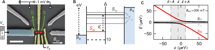
Figure 1: Experimental setup. (A) Scanning electron micrograph showing Ti/Au gates on the surface of a GaAs / AlGaAs heterostructure ($500\,$nm scale bar). Six of the Ti/Au gates (yellow) are used to laterally define a DQD in the 2DES 85 nm beneath the surface, the others are grounded. A cobalt single-domain nanomagnet (blue) produces an inhomogeneous magnetic field which slightly mixes singlet and triplet states of the DQD. (B) Typical situation in our two-electron DQD: vertical lines indicate tunable tunnel barriers, horizontal lines chemical potentials, blue areas the degenerate 2DES leads. The voltage $V=(\mu_{\text{S}}-\mu_{\text{D}})/e$ causes a single-electron tunneling current (green arrow in panel A). (C) Energy diagram of the relevant two-electron DQD eigenstates. Singlets (the qubit states) are represented as black and red lines; triplets, which are Zeeman split, as gray lines. Rf-modulation of the gate voltage $V_{\sim}$ (panel A) results in a modulated detuning $\epsilon(t)$, indicated by gray shading.

Source and drain leads at chemical potentials $\mu_{\text{S,D}}$, each tunnel coupled to one dot, allow current flow by single-electron tunneling. Applying the voltage $V=(\mu_{\text{S}}-\mu_{\text{D}})/e=1\,$mV across the DQD (Fig. 1B) we use this current to detect the steady-state properties of the driven system. We interprete the singlets, $\text{S}_{11}$ (one electron in each dot) and $\text{S}_{20}$ (two electrons in the left dot), as qubit states. They form an avoided crossing (Fig. 1C), described by the Hamiltonian

$$H_{\text{qubit}}=\begin{pmatrix}0&\Delta/2\\ \Delta/2&-\epsilon(t)\end{pmatrix}\,,$$ (1)

where we consider a variable energy detuning $\epsilon(t)$ and a constant inter-dot tunnel coupling tuned to $\Delta\simeq 13\,\mu$eV, corresponding to a clock speed of $\Delta/h\simeq 3.1\,$GHz, where $h$ is the Planck constant.

Let us first discuss a single sweep through the avoided crossing at $\epsilon=0$: as shown back in 1932 independently by Landau, Zener, Stückelberg, and Majorana it brings the qubit into a superposition state Landau1932a ; Zener1932a ; Stueckelberg1932a ; Majorana1932a , the electronic analog to the optical beam splitter. The probability to remain in the initial qubit state, $P_{\text{LZ}}=\exp(-\pi\Delta^{2}/2\hbar v)$, thereby grows with the velocity $v=\text{d}\epsilon/\text{d}t$, here assumed to be constant Landau1932a ; Zener1932a ; Stueckelberg1932a ; Majorana1932a . Because the relative phase between the split wavepackets depends on their energy evolutions, repeated passages by a periodic modulation $\epsilon(t)=\bar{\epsilon}+A\cos(\Omega t)$, give rise to so-called LZSM quantum interference Zener1932a ; Stueckelberg1932a ; Majorana1932a ; Oliver2005a ; Sillanpaa2006a ; Wilson2007b ; Berns2008a ; Shevchenko2010a ; Huang2011 ; Stehlik2012a ; Dupont-Ferrier2013 ; Cao2013 ; Nalbach2013 ; Ribeiro2013 . We present a breakthrough which makes LZSM interferometry a powerful tool: it is based on systematic measurements together with a realistic model, which explicitly includes the noisy environment. We demonstrate how to decipher the detailed qubit dynamics and directly determine its decoherence time $T_{2}$ based on straightforward steady state measurements.

Keeping the experiment simple we detect the dc-current $I$ through the DQD. It involves electron tunneling giving rise to the configuration cycle $(1,0)\to(1,1)\leftrightarrow(2,0)\to(1,0)$, where pairs of digits refer to the number of electrons charging the (left, right) dot (Fig. 1B). The energetically accessible two-electron states include the singlets $\text{S}_{11}$ and $\text{S}_{20}$ but also three triplets $\text{T}_{11}$ (Figs. 1B and C). These triplets are likely occupied during $(1,0)\to(1,1)$ and their decay via a spin-flip, $\text{T}_{11}$ $\to$ $\text{S}_{11}$, is hindered by Pauli-spin blockade Ciorga2000a ; Ono2002 . This suppresses the transition $(1,1)\to(2,0)$ and thereby limits the current. To nevertheless quickly initialize the qubit and generate a measurable current we lift the blockade using an on-chip nanomagnet (Fig. 1A) Petersen2013a . $I$ is proportional to the occupation probability of $\text{S}_{20}$ and serves as destructive qubit detector.

As it is possible to tune the relative couplings and the mean detuning $\bar{\epsilon}$ of the singlet-singlet and singlet-triplet crossings by gate voltages and magnetic fields, our two-electron DQD opens two interesting perspectives: (i) LZSM interferometry involving multiple avoided crossings and (ii) coherent Landau-Zener transitions between our charge qubit and the recently very successful spin-based qubits Bluhm2011 .

Concentrating on the two-electron charge qubit, in Figs. 2A and B we display LZSM interference patterns measured at $T_{\text{2DES}}\simeq 20\,\text{mK}$ for two different modulation frequencies $\Omega/2\pi$. Within the triangle defined by $A\gtrsim|\bar{\epsilon}|$, the qubit is periodically driven through the avoided crossing and the current oscillates between zero and distinct maxima indicating destructive and constructive interference Kayanuma1994a ; Shevchenko2010a . An interpretation based on photon-assisted tunneling (PAT), which is for $\hbar\Omega\gtrsim\Delta$ fully equivalent to the LZSM picture discussed above, facilitates quantitative predictions: using Floquet scattering theory Strass2005b we find

$$I(\bar{\epsilon},A)=\frac{e}{\hbar}\frac{\Gamma_{\text{in}}\Gamma_{\text{out}}}{4\gamma}\sum_{n=-\infty}^{\infty}\frac{\Delta_{n}^{2}}{(\bar{\epsilon}-n\hbar\Omega)^{2}+\Delta_{n}^{2}+\gamma^{2}}\,,$$ (2)

per spin projection, where $\Gamma_{\text{in}}$ is the qubit initialization rate $(1,0)\to\text{S}_{11}$ and $\Gamma_{\text{out}}$ the decay rate $(2,0)\to(1,0)$ and $\gamma=\frac{1}{2}(\Gamma_{\text{in}}+\Gamma_{\text{out}})$. The interdot tunnel coupling is renormalized with the $n$th-order Bessel function $J_{n}$ of the first kind: $\Delta_{n}=J_{n}(A/\hbar\Omega)\Delta$. Eq. (2) predicts Lorentz-shaped current maxima of width $\delta\bar{\epsilon}=\sqrt{\Delta_{n}^{2}+\gamma^{2}}$ at the $n$-photon resonances $\bar{\epsilon}=n\hbar\Omega$, modulated by $J_{n}^{2}(A/\hbar\Omega)$ as function of $A$. This scattering approach provides an appealing physical picture and describes the main features of the measured LZSM patterns as can be easily seen for the high frequency limit $\hbar\Omega\gg\delta\bar{\epsilon}$ (supplementary material: Fig. 9). For lower $\Omega$, the distance between current peaks is smaller and, hence, the broadened resonances tend to merge (Fig. 2A).

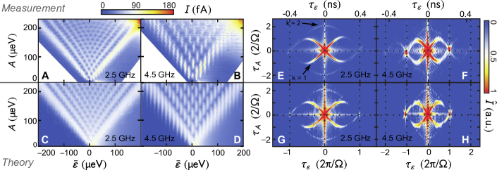
Figure 2: LZSM interference. (A and B) Measured current through the DQD as a function of mean detuning $\bar{\epsilon}$ and modulation amplitude $A$ for two modulation frequencies at $T\simeq 20\,$mK. (C and D) Same as (A) and (B) but numerically calculated for realistic conditions. (E–H) Two-dimensional numerical Fourier transformed ($A\to\tau_{A}$, $\bar{\epsilon}\to\tau_{\epsilon}$, $I\to\widehat{I}$) of measurements (upper panels) and theory (lower panels). The shape of the sinusoidal branches of enhanced $\widehat{I}$ is determined by $\Omega$, see Eq. (3). Their decay with increasing $\tau_{\epsilon}$ encodes dephasing and decoherence. The horizontal and vertical lines of enhanced amplitude at $\tau_{A}=0$ and $\tau_{\epsilon}=0$ are artefacts caused by the finite region of data being transformed.

The visibility of the LZSM pattern (i) depends on frequency and amplitude via the Landau-Zener probability $P_{\text{LZ}}$ (captured in Eq. (2) by $\Delta_{n}$), is (ii) strongest for $\Gamma_{\text{in}}\simeq\Gamma_{\text{out}}$ and is (iii) diminished for $\Delta<\gamma$, where the qubit decay is faster than its clock-speed. However, Eq. (2) fails to predict the qubit coherence time as it ignores environmental noise. The nevertheless qualitative consent indicates that environmental noise can be treated perturbatively. In this spirit, we developed a complete model which goes beyond Eq. (2) by explicitly including all energetically accessible states of our driven DQD and, importantly, decoherence within a system-bath approach.

An evident source of decoherence is the interaction of the qubit electrons with bulk phonons Granger2012a which entails quantum fluctuations to the DQD level energies. It enters our theory as dissipation kernel with a dimensionless electron-phonon coupling strength $\alpha_{Z}$ (supplementary material: B.1, B.2) derived from a system-bath approach becoming the spin-boson model in the qubit subspace Hanggi1990a ; Makhlin2001b . We assume for the coupling an Ohmic spectral density which is justified by geometry considerations (supplementary material: B.1.3) and also a posteriori by a surprisingly good agreement with our experimental results.

The second environmental component of our model is charge noise, well known to cause low frequency fluctuations of the local confinement potential in semiconductor heterostructures Fujisawa2000 ; Pioro-Ladriere2005 ; Buizert2008 ; Yacoby2013 . Being slow compared to all relevant time scales of our experiment, they can be treated as static disorder leading in the ensemble average to an inhomogeneous, Gaussian broadening of width $\lambda^{\star}$.

To determine the key parameters $\lambda^{\star}$ and $\alpha_{Z}$ we solve the Bloch-Redfield master equation self-consistently using Floquet theory and numerically model our data (supplementary material: B.3) The optimized result is displayed in Figs. 2C and D with $\lambda^{\star}=3.5\,\mu$eV and $\alpha_{Z}=1.5\cdot 10^{-4}$. Below, we illustrate the self-consistent procedure by first determining $\lambda^{\star}$ based on the final value of $\alpha_{Z}$ and then evaluating $\alpha_{Z}$ using the final value of $\lambda^{\star}$.

Fig. 4A displays $I(\bar{\epsilon})$ for $\Omega/2\pi=2.75\,$GHz and a constant $A$, corresponding to a horizontal slice in the presentations of Figs. 2A–D. The measured data (dots) in Fig. 4A feature a beating of broadened and overlapping current peaks. The gray line is calculated for $\alpha_{Z}=1.5\cdot 10^{-4}$ and $\lambda^{\star}=0$. Compared to our measurement it shows a weaker broadening and a higher visibility. Much better agreement is reached for $\lambda^{\star}=3.5\,\mu$eV (blue line). This result is robust under moderate variations of $\alpha_{Z}$ and does not depend on frequency or temperature. Fig. 4B underlines the good agreement between measured (dots) versus calculated (lines) data by presenting $I(A)$ at $\bar{\epsilon}=n\hbar\Omega$ for various $n$ (vertical slices in Figs. 2A–D). Owing to the electron-phonon interaction, the visibility of the interference pattern drops with increasing temperature (Fig. 4C).

To quantify $\alpha_{Z}$ with high accuracy, we use this temperature dependence and thereby capture global information of the extended LZSM patterns (Figs. 2A–D) by performing two-dimensional Fourier transformations $I(\bar{\epsilon},A)\to\widehat{I}(\tau_{\epsilon},\tau_{A})$. The result, featured in Figs. 2E–H, are simple, lemon-shaped structures of local maxima $\widehat{I}(\tau_{\epsilon},\tau_{A})\big{|}_{\text{lemon}}$. Transforming Eq. (2) yields an analytic formula describing these lemon arcs:

$$\tau_{A}=\pm\frac{2k}{\Omega}\sin\bigg{(}\frac{\Omega\tau_{\epsilon}+2\pi k^{\prime}}{2k}\bigg{)},$$ (3)

with $k=1,2,3,\dots$, $k^{\prime}=0,1,2,\dots$ and $k^{\prime}<k$. Arcs for $k>1$ are a consequence of $\Delta\gtrsim\gamma$, a prerequisite for observing a pronounced interference pattern (supplementary material: A.5). (Arcs for $k>1$ are weakly seen in Figs. 2E–H. In superconducting qubits they have been also observed but—considering $\Delta\ll\gamma$ Rudner2008a —not explained.) Concentrating on the principal lemon arc for $k=1$, we find a non-monotonic behavior of $\widehat{I}(\tau_{\epsilon},\tau_{A})\big{|}_{\text{lemon}}$ with maxima at the arc’s intersections (at $\tau_{A}=0$ and $\tau_{\epsilon}$ a multiple of $2\pi/\Omega$). Regions of decays in-between have the form

$$\widehat{I}(\tau_{\epsilon},\tau_{A})\big{|}_{\text{lemon}}\propto e^{-\lambda\left|\tau_{\epsilon}\right|/\hbar}\,e^{-\frac{1}{2}(\lambda^{\star}\tau_{\epsilon}/\hbar)^{2}}\,,$$ (4)

where the exponential term originates from the Lorentzian broadening due to electron-phonon coupling and the Gaussian term describes the inhomogeneous broadening caused by charge noise. Notice that $\tau_{\epsilon}$ is a Fourier variable rather than a real time and, thus, $\lambda$ should not be interpreted as physical decay rate. (Only for $\Delta\ll\gamma$, all Lorentzians in Eq. (2) possess the same width, so that $\widehat{I}(\tau_{\epsilon},\tau_{A})\big{|}_{\text{lemon}}$ is described by Eq. (4) with simply $\lambda=\gamma$ as suggested in Ref. Rudner2008a .) In Figs. 4A and C

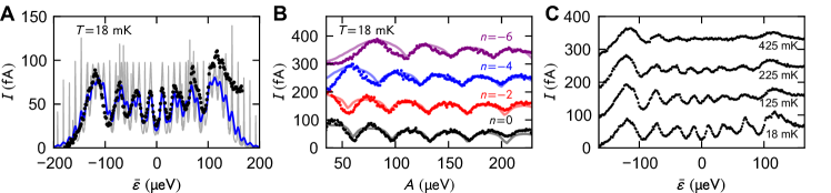
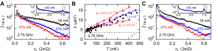
Figure 3: Raw data analysis. Dots are measured at $\Omega/2\pi=2.75\,$GHz, lines numerical data for $\alpha_{Z}=1.5\cdot 10^{-4}$ and $\lambda^{\star}=3.5\,\mu$eV, only the gray line in panel A is for $\lambda^{\star}=0$. (A) Horizontal slice through a LZSM pattern: $I(\bar{\epsilon})$ for a constant $A=130\,\mu$eV. (B) Vertical slices through a LZSM pattern: $I(A)$ for $\bar{\epsilon}/(\hbar\Omega)=0$, $-2$, $-4$, $-6$. (C) Measured data as in panel A for various temperatures.

Figure 4: Electron-phonon coupling. (A) Decaying region of the measured $\widehat{I}(\tau_{\epsilon},\tau_{A})\big{|}_{\text{lemon}}$ for three temperatures (dots). Lines are generated using Eq. (4) for $\lambda^{\star}=3.5\,\mu$eV and $\lambda$ as a fit parameter. The inset shows a broader region including maxima at $\tau_{\epsilon}=0$, $2\pi/\Omega$. (B) Measured decay rate $\lambda(T)$ (black) and corresponding numerical data (colored) based on $\lambda^{\star}=3.5\,\mu$eV (indicated as horizontal line) and $\alpha_{Z}=1.0$, $1.5$, $2.0\times 10^{-4}$. (C) Analog to panel A but based on numerical calculations. Solid lines are identical to those in A. The numerical resolution is based on 100 data points sampling the Gaussian broadening in $\bar{\epsilon}$ of width $\lambda^{\star}=3.5\,\mu$eV.

we plot measured and calculated decays (dots), respectively, for various temperatures between 18 mK and 500 mK. The solid lines in panels A and C are identical and express Eq. (4) with $\lambda$ as fit parameter, while $\lambda^{\star}$ is kept fixed at $3.5\,\mu$eV. Fig. 4B compares $\lambda(T)$ obtained by this procedure from our measurements (black dots) with the numerical results using three different values of $\alpha_{Z}$. An outstanding agreement between theory and experiments is found at $\alpha_{Z}\simeq 1.5\cdot 10^{-4}$ (blue in Fig. 4B). This completes our set of model parameters needed to calculate LZSM patterns as in Figs. 2C and D. $\lambda(T)$ increases linearly for $T\gtrsim 100\,$mK, while it is bounded by $\lambda_{\text{min}}\simeq 4\,\mu$eV at our lowest temperatures. This bound marks the intrinsic decay of $\widehat{I}(\tau_{\epsilon},\tau_{A})\big{|}_{\text{lemon}}$ present even in the low-temperature limit of our transport measurement but is not related to the low temperature bound of the coherence time $T_{2}$.

To actually identify $T_{2}(T)$ we use its dependence on $\alpha_{Z}$ in the spin-boson model. In the absence of rf-modulation, it provides the analytical prediction weiss89 ; Makhlin2001b :

$$T_{2}(T,\alpha_{Z})=\frac{\hbar}{\pi\alpha_{Z}}\left(\frac{2k_{\text{B}}T\bar{\epsilon}^{2}}{E^{2}}+\frac{\Delta^{2}}{2E}\coth\left(\frac{E}{2k_{\text{B}}T}\right)\right)^{-1}\,.$$ (5)

In the low temperature limit, $k_{\text{B}}T\ll E=\sqrt{\Delta^{2}+\bar{\epsilon}^{2}}$ our undriven qubit has, $T_{2}=2\hbar E/\pi\alpha_{Z}\Delta^{2}$. Assuming $\bar{\epsilon}=0$ we find $T_{2}\simeq 0.2\,\mu$s, which further increases at finite detuning. Alternatively, $T_{2}$ could be increased by decreasing $\Delta$. This would, however, reduce the clock-speed of the qubit. In the same spirit, the rf-induced renormalization of $\Delta\to\Delta_{n}$ stabilizes the qubit’s coherence on the expense of a larger gate operation time Fonseca2004a .

Summarizing, we demonstrated that steady-state LZSM interferometry is a viable tool to fully characterize a qubit including its coupling to a noisy environment. The quantitative agreement between our experiments and our complete system bath model analyzed with Floquet transport theory allows us to trace the origins of inhomogeneous broadening and decoherence. Thereby we determined the individual values of $T_{2}^{\star}$ and $T_{2}$ of the qubit. Our steady-state method is remarkably simple compared to the alternative pulsed gate experiments. Our two-electron charge qubit is affected by slow charge noise limiting $T_{2}^{\star}=\hbar/\lambda^{\star}$ to $\simeq 0.2\,$ns but a coherence time of $T_{2}\simeq 0.2\,\mu$s being much longer than previously reported values in quantum dot charge qubits Hayashi2003a ; Petersson2010a ; Cao2013 . The clock-speed of our qubit, $\Delta/h\simeq 3.1\,$GHz, which limits $T_{2}$ at $T\simeq 20\,$mK and $\bar{\epsilon}=0$, would then provide enough time for $>600$ quantum operations. At higher temperatures or sizable $\bar{\epsilon}$ the decoherence is dominated by the electron-phonon coupling. Our method is simple, very general and can be applied to arbitrary qubit systems. An extension including individually controlled Landau-Zener transitions and a combination with non-adiabatic pulses will open up alternative means of quantum information processing. Our two-electron qubit experiments illustrate an interesting approach for studying the interaction of qubits and complex many body quantum systems.

Author contributions

S. L. initiated and supervised the project. S. K. developed and implemented the theoretical model and performed the numerical calculations. G. P. fabricated the DQD sample. G. P. and F. F. performed the experiments. D. S. and W. W. provided the wafer material. S. M. helped to develop the high frequency setup. S. K., G. P., F. F., P. H. and S. L. analyzed the data and wrote the manuscript.

METHODS

Experiment: The sample is based on a GaAs / AlGaAs heterostructure, grown by molecular beam epitaxy, with a 2DES situated $85\text{\,}\mathrm{nm}$ beneath the surface. After the 2DES has been characterized at $T=$4.2\text{\,}\mathrm{K}$$, at which temperature the carrier density is $n_{\text{e}}=$1.19\text{\times}{10}^{11}\text{\,}{\mathrm{cm}}^{-2}$$ and the mobility is $\mu=$0.36\text{\times}{10}^{6}\text{\,}{\mathrm{cm}}^{2}\text{\,}{\mathrm{V}}^{-1}\text{\,}{\mathrm{s}}^{-1}$$, we used electron-beam lithography to fabricate the nanostructure. The metal gates in Fig. 1 contain 30 nm of gold on top of 5 nm of titanium. The DQD is defined electrostatically by applying negative voltages to these gates and tuned to the ground state configuration (1,1) (one electron per dot). The inhomogeneous field of an on-chip nanomagnet partly lifts the Pauli-spin blockade (detailed in reference Petersen2013a ) and allows LZSM measurements in the most interesting regime where charge and spin qubits can coexist. Here we concentrate on a charge qubit and measure a single-electron-tunneling dc current through the DQD while the voltage on one gate is modulated at radio frequencies (Fig. 1). More details on the DQD configuration, the measurements and the data analysis are provided in the supplementary material: A.

Theory: With our model we aim at realistic predictions for the dc current $I(\bar{\epsilon},A)$ through the DQD. It takes into account the nine most relevant energy states for the charge configurations (1,0), (2,0), (1,1), and (2,1) of the DQD Hilbert space, which are the states with chemical potentials lying between or close to those of the source and drain leads. The Hamiltonian includes inter-dot and dot-lead tunneling, inter- and intra-dot Coulomb repulsion, Zeeman terms stemming from an inhomogeneous magnetic field and the modulation of the on-site energies by applying an rf voltage to one gate. For the coupling to the dissipative environment we employ a generalized spin-boson model. To describe the periodically driven quantum system we use Floquet theory which is based on the ansatz $\psi_{n}(t)=e^{-i\omega_{n}t}\phi_{n}(t)$ with $\phi_{n}(t)=\phi_{n}(t+2\pi/\Omega)$ resembling Bloch-functions but with the space coordinate replaced by time, while the quasi-energy $\hbar\omega_{n}$ corresponds to the quasi-momentum. We then include the dot-lead tunneling and the action of the dissipating environments within Bloch-Redfield theory. Using the Floquet states as basis captures the influence of the rf-field and allows us to treat the resulting master equation within a rotating-wave approximation. This offers an important computational advantage because finding the steady-state solution is now reduced to solving a linear, time-independent matrix equation, despite the rf driving Kohler2005a . Our experimental results do not indicate any significant temperature dependence of the spin relaxation time (within the temperature window explored). Therefore, we treat the latter in a simplified way using a Lindblad form with a phenomenological rate. Finally, we identify the current operator: it corresponds to those terms of the master equation describing the incoherent transition $(2,0)\to(1,0)$, i. e. the tunneling of electrons from the left dot to the drain lead. The measured dc current corresponds to the expectation value of the current operator. More details of our theory are provided in the supplementary material: B.

SUPPLEMENTARY INFORMATION

In the main article we demonstrated that LZSM interferometry is a viable tool to measure standard qubit properties and, beyond, to determine its coupling to a noisy environment. In our specific case of a DQD charge qubit we found two main noise sources: (i) slow environmental fluctuations resulting in an inhomogeneous Gaussian broadening, and (ii) the heat bath, resulting in a homogeneous Lorentzian broadening. In Appendix A we provide additional experimental results together with numerical data, which underlie our interpretations in the main article. Further, we detail our quantitative data analysis based on a self-consistent fitting procedure and numerical calculations resulting in the qubit-environment coupling constants, namely the standard deviation $\lambda^{\star}=\hbar/T_{2}^{\star}$ of the inhomogeneous broadening and the dimensionless dissipation strength $\alpha_{Z}$ of the coupling to the phonons.

In Appendix B we discuss the details of our model for the DQD and its coupling to the leads as well as to the phonons. Moreover, we sketch the Bloch-Redfield master equation approach by which we compute the asymptotic state of the DQD and the time-averaged current. This includes a discussion of how we extract the qubit’s coherence time $T_{2}$ from $\alpha_{Z}$ and under which conditions this is an appropriate procedure. Note that we neglect a second component of the electron-phonon coupling, namely $\alpha_{X}$ which would mainly cause additional energy relaxation between the qubit states. An estimate of $\alpha_{X}$ and a discussion, which justifies its negligence, is provided in Appendix B.

Table 1 in Appendix C summarizes all system parameters extracted from various measurements and used for the numerical calculations.

Appendix A Additional Experiments and Data Analysis

A.1 Initial tuning of the double quantum dot

Our experiments start by tuning the double quantum dot (DQD) by means of gate voltages. As an orientation, Fig. 5A

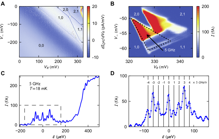
Figure 5: Initial tuning of the qubit. (A) Charge stability diagram of the unbiased DQD ($V=0$) as function of dc gate voltages (the gates are marked in Fig. 1A), measured by charge detection Field1993 at $T\simeq 20\,$mK. In detail, the color scale displays the linear transconductance of a nearby almost pinched off quantum point contact. It has been defined in the 2DES by $V_{\sim}$ and the upper left gate (gray in Fig. 1A). Sharp lines of minimal transconductance are charging lines of the DQD which is empty [configuration $(0,0)$] in the lower left half of the plot. (B) Current $I$ in the vicinity of the $(1,1)\leftrightarrow(2,0)$ transition of the charge stability diagram for $V=1\,$mV applied across the DQD (see Fig. 1A) while $V_{\sim}$ was modulated with frequency $\Omega/2\pi=5\,$GHz and amplitude $A\simeq 80\,\mu$eV. The dashed triangle marks the region of current via $(1,0)\to(2,0)\leftrightarrow(1,1)\to(1,0)$. The black arrow indicates the detuning axis $\bar{\epsilon}$ and $\bar{\epsilon}=0$ at its intersection with the dashed line. (C) $I(\bar{\epsilon})$ measured along the black arrow in (B). (D) Current around $\bar{\epsilon}=0$ corresponding to the region framed by a dashed box in (C). The current maxima at $\bar{\epsilon}=n\hbar\Omega$ with $n=0,\pm 1,\pm 2,\pm 3,\pm 4$ (vertical lines) are caused by PAT.

displays a charge stability diagram of the unbiased DQD ($V=0$) as function of the gate voltages $V_{\sim}$ and $V_{\text{R}}$. It has been measured using a QPC as charge detector. The sharp lines of local minima in transconductance $\text{d}I_{\text{QPC}}/\text{d}V_{R}$ are the charging lines of the two dots which separate regions of stable charge configurations ranging from $(0,0)$ to $(2,1)$. Fig. 5B details the region of the stability diagram near the transition $(1,1)\leftrightarrow(2,0)$, but it plots the current $I$ measured through the DQD as a response to $V=1\,$mV applied across the DQD (see Figs. 1A and B). The finite current within the framed triangle is a consequence of the single-electron tunneling cycle $(1,0)\to(1,1)\leftrightarrow(2,0)\to(1,0)$, where the double arrow accounts for the fact that the interdot tunnel coupling is coherent and large compared to the dot-lead tunnel couplings. The transition $(1,1)\leftrightarrow(2,0)$ thereby divides into $\text{S}_{11}\leftrightarrow\text{S}_{20}$ and $\text{T}_{11}\leftrightarrow\text{T}_{20}$ while the coupling between singlet and triplet subspaces is forbidden by the Pauli principle. This is the configuration used for our LZSM interferometry measurements. The black arrow in Fig. 5B indicates the detuning axis. The current along this arrow, i. e. as a function of mean detuning $\bar{\epsilon}$, plotted in Fig. 5C, shows two interesting features: (i) $I$ is strongly suppressed for $\bar{\epsilon}<400\,\mu$eV, because there the $\text{T}_{20}$ state is beyond the transport window, while the transition $\text{T}_{11}\to\text{S}_{11}$ is hindered by Pauli-spin blockade Ciorga2000a ; Ono2002 , which makes $\text{T}_{11}$ a metastable state. In our case the spin blockade is partly lifted especially near $\bar{\epsilon}=0$ where the inhomogeneous field of our nanomagnet mixes $\text{T}_{11}$ and $\text{S}_{11}$; spin relaxation, provided by the hyperfine interaction with nuclear spins Petersen2013a also contributes, but is weaker. The strong current increase at $\bar{\epsilon}\simeq 400\,\mu$eV marks the onset of the $\text{T}_{20}$ state contributing to the transport which then completely lifts the spin blockade via the triplet channel $(1,0)\to\text{T}_{11}\leftrightarrow\text{T}_{20}\to(1,0)$. (ii) In Fig. 5B we have, in addition, applied an rf-modulation of $V_{\sim}$ at the frequency of 5 GHz resulting in a modulation of the detuning with amplitude $A\simeq 80\,\mu$eV. This gives rise to a pattern of photon assisted tunneling (PAT) current maxima appearing at $\bar{\epsilon}=n\hbar\Omega$ with $n=0,\pm 1,\pm 2,\dots$. These PAT peaks in $I(\bar{\epsilon})$, highlighted in Fig. 5C, transform into the LZSM patterns observed in our 2D plots $I(\bar{\epsilon},A)$. Weaker PAT oscillations are also seen in panel C where the $\text{T}_{20}$-triplet starts to contribute to the current near $\bar{\epsilon}\simeq 400\,\mu$eV. (The actual singlet-triplet splitting in the $(2,0)$-configuration is larger by the amplitude of $A=80\,\mu$eV and accounts to $\simeq 480\,\mu$eV.)

An example of measured LZSM interferometry is displayed in Fig. 6

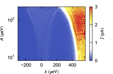
Figure 6: LZSM patterns: singlets versus triplets. $I(\bar{\epsilon},A)$ at $\Omega/2\pi=2.5\,$GHz and $T\simeq 20\,$mK (logarithmic amplitude axis). Not only for the singlets transition $\text{S}_{11}\leftrightarrow\text{S}_{20}$ (left) but also for the triplets transition $\text{T}_{11}\leftrightarrow\text{T}_{20}$ (right) is a LZSM interference pattern observed.

using a logarithmic $A$-axis. It clearly shows LZSM interference patterns involving both transitions $\text{S}_{11}\leftrightarrow\text{S}_{20}$ around $\bar{\epsilon}=0$ as well as $\text{T}_{11}\leftrightarrow\text{T}_{20}$ at larger $\bar{\epsilon}$ where the $\text{T}_{20}$ state contributes to transport. In all other LZSM patterns presented in this article, the color scale is chosen to optimize the singlet contributions to the interference and the onset of the triplet channel is only seen as an asymmetry in $I(\bar{\epsilon})$ at large $A$ (increased current in the upper right corner of e. g. Figs. 2A and B).

A.2 Energy calibration

In this section we briefly explain how we determine the detuning $\bar{\epsilon}$ and the modulation amplitude $A$ from gate voltages, the source-drain voltage $V$ applied across the DQD and the modulation frequency $\Omega$. The standard method is to use the current triangles in Fig. 5B which relate the known energy scale of the applied source-drain voltage $eV$ to changes in gate voltages $V_{\sim}$ and $V_{R}$. The relations are linear with the mutual gate-dot capacities as proportionality factors Taubert2011a . Here, we can refine such a standard calibration based on the well known modulation frequency, which determines the LZSM interference patterns, in the following way: (i) The current maxima appear at $\bar{\epsilon}=n\hbar\Omega$ with $n=0,1,2,\dots$ which we use to calibrate $\bar{\epsilon}(V_{R},V_{\sim})$. (ii) The positions of the minima of the current as function of amplitude are also well known (see e. g. Eq. (2)) and we use them to calibrate $A(V_{R},V_{\sim})$. At small frequencies, where the interference patterns are less clear, the positions of the outermost current maxima (at $A\simeq\bar{\epsilon}$) framing the region of finite current $I(\bar{\epsilon},A)$ (e. g. in Figs. 2A and B) can still be used for a calibration. As the transmission of the rf modulation to the sample depends on the frequency due to cable resonances in the experimental setup, the calibration of $A$ has to be done separately for each frequency.

A.3 Determination of the system parameters

Using our model we aim at a quantitative prediction of the measured current. This requires knowledge of various system parameters such as the tunable tunnel barriers and transition rates between triplet and singlet states. All parameters used in our numerical calculations are summarized for convenience in Table 1 in Appendix C. Following, we describe our determination of those parameters, which are neither trivial nor described elsewhere in this article. The largest energy scales are the intradot and interdot Coulomb interactions $U\simeq 3.5\,$meV and $U^{\prime}\simeq 0.8\,$meV. Knowing the energy calibration (see last section) these values can be extracted from charge stability diagram. In detail, $U$ corresponds to the distance between charging lines in Fig. 5A and $U^{\prime}$ to the distance between the triangle tips in Fig. 5B. Next, we discuss the triplet-singlet coupling, which in our case originates from the hyperfine interaction between the electrons and many nuclei on the one hand and the inhomogeneous magnetic field of our nanomagnet, shown in Fig. 1A, on the other hand. The $\text{T}_{11}$ triplets split into $T_{+}=\left|\uparrow\uparrow\right>$, $T_{0}=\left(\left|\uparrow\downarrow\right>+\left|\downarrow\uparrow\right>\right)/\sqrt{2}$ and $T_{-}=\left|\downarrow\downarrow\right>$. The couplings between $T_{+}$ and $\text{S}_{11}$ and between $T_{-}$ and $\text{S}_{11}$ are identical and caused by field inhomogeneities parallel to the effective magnetic field (approximately parallel to $B_{\text{ext}}=200\,$mT, see Figs. 1A and C), while $T_{0}$ and $\text{S}_{11}$ are coupled by the perpendicular field inhomogeneities. We actually determine the $T_{+}$-$\text{S}_{11}$ coupling by measuring the average charge occupation in a continuously pulsed gate experiment. Here, we use a quantum point contact as charge detector (while no voltage is applied across the DQD, $V=0$). As sketched in the inset of Fig. 7A and in the energy diagram in Fig. 7D,

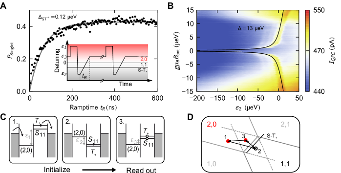
Figure 7: Singlet-triplet and interdot tunnel couplings. (A) Probability to occupy the singlet state $\text{S}_{11}$ after initialization in the same state and then sweeping across the $\text{S}_{11}$-$T_{+}$ avoided crossing (at $T\simeq 20\,$mK) as a function of the ramp time $t_{\text{R}}$ which is proportional to the inverse sweep speed $v$. From the theory (gray line) the singlet-triplet coupling is determined (details in bulk text). The inset sketches the pulse sequence. (B) Current $I_{\text{QPC}}$, measured at $T\simeq 20\,$mK through the detector quantum point contact, as function of an external magnetic field and detuning $\epsilon_{2}$, where the entire pulse sequence shown in the inset of panel A is shifted vertically. Otherwise, the applied pulse sequence is the same as in A, but with a quick and constant ramp time $t_{\text{R}}\simeq 1.1\,$ns. Enhanced current at the black lines (theory) mark singlet-triplet resonances. This so-called spin-funnel is used to determine the interdot-tunnel coupling $\Delta$ (details in bulk text). (C) Subfigures 1., 2., 3. sketch the chemical potentials (and dynamics) of the DQD at detunings $\epsilon_{1}$, $\epsilon_{2}$, $\epsilon_{3}$ in the inset of panel A. (D) Sketch of the DQD charge stability diagram indicating the positions at detunings $\epsilon_{1}$, $\epsilon_{2}$, $\epsilon_{3}$ during the pulse sequence sketched in the inset of panel A.

we first initialize the DQD in $\text{S}_{20}$ by applying a large positive detuning $\epsilon_{1}$ (where the transition $\text{T}_{11}\to\text{S}_{20}$ happens quickly via charge exchange with the leads: $\text{T}_{11}\to(1,0)\to\text{S}_{20}$; see left panel in Fig. 7C). Next we prepare the DQD in the $\text{S}_{11}$-state at $\epsilon=\epsilon_{2}$ by sweeping the detuning from $\epsilon_{1}\to\epsilon_{2}$ at a constant speed obeying $\Delta^{2}\gg 2\hbar v/\pi\gg\Delta_{\text{ST},\pm}^{2}$. During this sweep, the DQD is adiabatically transferred from the $\text{S}_{20}$ to the $\text{S}_{11}$ state while passing the $\text{S}_{20}$-$\text{S}_{11}$ avoided crossing with coupling $\Delta$. The DQD also passes the $\text{S}_{11}$-$T_{+}$ avoided crossing with coupling $\Delta_{\text{ST},\pm}$; this passage is, however, non-adiabatic because $\Delta_{\text{ST},\pm}\ll\Delta$ and, hence, the DQD remains in the $\text{S}_{11}$-state. After waiting a short time at $\epsilon_{2}$ (center panel in Fig. 7C), we perform a Landau-Zener passage within the ramp time $t_{\text{R}}$ through the $\text{S}_{11}$-$T_{+}$ avoided crossing up to $\epsilon=\epsilon_{3}$ where we spend a relatively long time in order to read out the charge state of the DQD (right panel in Fig. 7C). We expect to find $(2,0)$ in case of a slow passage (with the DQD staying in the singlet subspace) and $(1,1)$ in case of a fast passage bringing the DQD into the $T_{+}$ state, because the decay $T_{+}\to\text{S}_{11}\to\text{S}_{20}$ is hindered by Pauli-spin blockade. Fig. 7A displays the probability to stay in the singlet subspace $P_{\text{singlet}}=\alpha\left(1-P_{\text{LZ}}\right)=\alpha\left(1-\text{exp}\left[-\pi\Delta_{\text{ST},\pm}^{2}/2\hbar v\right]\right)$ as a function of $t_{\text{R}}=(\epsilon_{3}-\epsilon_{2})/v$. Fitting this function (gray line in Fig. 7A) to the measured singlet probability indicates our $\text{S}_{11}$-$T_{+}$ coupling of $\Delta_{\text{ST},\pm}=(119\pm 10)\,$neV, produced by our nanomagnet. The pre-factor $\alpha\simeq 0.43$ accounts for the partial decay $T_{+}\to\text{S}_{11}$ and depends on the duration of the readout period. Taking into account the interdot tunnel coupling which results in a reduced weight of $\text{S}_{11}$ in the singlet eigenstate, this $\Delta_{\text{ST},\pm}$ corresponds to a magnetic field difference in the two dots giving rise to $g\mu_{\text{B}}\Delta B_{x}\simeq 0.2\,\mu$eV, smaller than previously measured in the same sample Petersen2013a , which indicates a degradation by oxidation of the single domain properties of our nanomagnet during six months of shelf storage. Here, we used the g-factor $|g|=0.36$ as determined for our DQD in Ref. Petersen2013a and Bohr’s magneton $\mu_{\text{B}}$. The hyperfine induced coupling contribution in our DQD is $\Delta_{\text{hyperfine}}\simeq 60\,$neV Petersen2013a and results in a corresponding inhomogeneous broadening of the singlet-triplet coupling.

To determine the interdot tunnel coupling $\Delta$ we perform a so-called spin funnel experiment Petta2005 . Thereby we repeat the same continuously pulsed gate measurements as above but with a short and fixed $t_{\text{R}}=1.1\,$ns so that all passages through the $\text{S}_{11}$-$T_{+}$ crossing are now equally non-adiabatic while the passage through the $\text{S}_{11}$-$\text{S}_{20}$ crossing is still adiabatic (see inset of Fig. 7A). Under this conditions, a pulse cycle $\epsilon_{1}\to\epsilon_{3}\to\epsilon_{2}\to\epsilon_{3}$ (Fig. 7D) will usually bring the system back to the $\text{S}_{20}$ singlet after preparing the $\text{S}_{20}$ singlet at the detuning $\epsilon_{1}$. A notable exemption occurs if $\epsilon_{2}$ coincides with the singlet-triplet resonance, namely for $\pm g\mu_{\text{B}}B_{\text{ext}}=\frac{1}{2}\left(\pm\sqrt{\epsilon_{2}^{2}+\Delta^{2}}-\epsilon_{2}\right)$, and if the system spends sufficient time ($>h/\Delta_{\text{ST}}$) there to allow for a singlet-triplet transition. As a consequence, we measure a deviation from the $\text{S}_{20}$ configuration at this resonance during the readout at $\epsilon_{3}$, where the $\text{T}_{11}$ triplet decays only slowly. To map out this condition we plot in Fig. 7C the current $I_{\text{QPC}}$ through the detector QPC (corresponding to the average charge state of the DQD) as a function of $g\mu_{\text{B}}B_{\text{ext}}$ and $\epsilon_{2}$. The two distinct lines of enhanced $I_{\text{QPC}}$ correspond to a finite occupation of one of the $T^{\pm}$ triplets. By fitting the resonance condition (above) we find our tunnel coupling $\Delta=(13\pm 1)\,\mu$eV (black lines in Fig. 7C).

The initialization and decay rates $\Gamma_{\text{in}}$ and $\Gamma_{\text{out}}$, respectively, are finally reconstructed from measuring the dc current through the DQD as a function of detuning and as a function of source drain voltage in forward and backward direction. An example of such a measurement is shown in Fig. 5C, where in this case an rf-modulation was applied in addition. Since the current in backward direction (for $\mu_{\text{D}}>\mu_{\text{S}}$ in Fig. 1B) is practically independent of the spin relaxation, it allows us to determine the dot-drain coupling $\Gamma_{\text{out}}=\Gamma_{L}$. In turn, the magnitude of the current in forward direction provides a faithful estimate for $\gamma_{\sigma}$ and $\Gamma_{\text{in}}$.

A.4 Origin of the inhomogeneous broadening

Compared to the measured LZSM patterns, our Floquet-Bloch-Redfield formalism, which already takes into account the realistic electron-phonon coupling $\alpha_{Z}$ (and the DQD parameters summarized in Table 1 such as tunnel couplings), predicts a much higher visibility of the interference pattern resulting in sharper current maxima. This is evident in Fig. 4A which compares the measured interference at a constant modulation amplitude with calculated data. We resolved this caveat by introducing an additional Gaussian inhomogeneous broadening $\lambda^{\star}$ (Fig. 4A), where the final values $\alpha_{Z}=1.5\times 10^{-4}$ and $\lambda^{\star}=3.5\,\mu$eV have been calculated self-consistently. Fig. 8

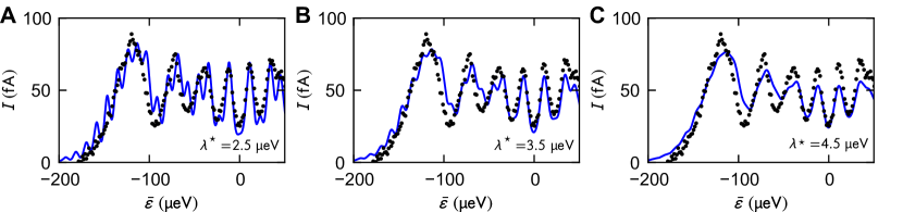
Figure 8: Accuracy in determination of inhomogeneous broadening. $I(\bar{\epsilon})$ at constant amplitude $A=130\,\mu$eV and for $T=18\,$mK and $\Omega/2\pi=2.75\,$GHz as in Fig. 4A. The measured data (black dots) are identical in all three panels while the model curves (blue lines) are based on the same $\alpha_{Z}=1.5\times 10^{-4}$ (our final value) but use various values of $\lambda^{\star}$. Best agreement with the measured data is reached for $\lambda^{\star}=3.5\,\mu$eV (panel B).

demonstrates the convergence by plotting three calculated curves (lines) using various values of $\lambda^{\star}$ around its final value while the electron-phonon coupling is kept fixed at $\alpha_{Z}=1.5\times 10^{-4}$ (as also in Fig. 4A). The model curve (blue line) in panel B using $\lambda^{\star}=3.5\,\mu$eV fits best to the measured data (dots).

The inhomogeneous broadening is a result of the combination of slow charge noise and our time averaging dc measurement: The spectrum of charge noise has been measured in heterostructures similar to ours. It can be described as $1/f$-noise which typically occurs only at frequencies below 10 kHz Fujisawa2000 ; Pioro-Ladriere2005 ; Buizert2008 ; Yacoby2013 . The longest time scale of our experiment is the dwell time in the DQD of each electron, contributing to the measured current. It is in the order of $1\,\mu$s, much shorter than the highest frequency components of charge noise. A single shot qubit measurement and hence $T_{2}$ is, consequently, unlikely to be affected by charge noise. However, in our steady state experiments each measured data point averages the dc current over $200\,$ms. Such an effective time ensemble measurement can be inhomogeneously broadened by charge noise, slow compared to $T_{2}$ but fast compared to the averaging time. Assuming a Markovian statistics, this inhomogeneous broadening is well described using a Gaussian distribution with standard deviation $\lambda^{\star}$.

A.5 Dissipation strength

In comparison, determining the dissipation parameter $\alpha_{Z}$ requires considerably more effort, experimentally and even more in theory, where it enters in a rather complex manner. We follow a route that is based on an idea by Rudner et al. Rudner2008a , who showed analytically that the Fourier transformed $\widehat{I}(\tau_{\epsilon},\tau_{A})$ of the dc current pattern exhibits a lemon-shaped structure, composed of sinusoidal branches. However, the treatment of Ref. Rudner2008a neglects the impact of the tunnel matrix element $\Delta$ on the dynamical phase which finally yields an expression similar to our Eq. (2), but with $\Delta_{n}^{2}+\gamma^{2}$ in its denominator replaced by a phenomenological decay rate $\widetilde{\gamma}^{2}$. Thus, the result is a simple Lorentzian broadening of width $\widetilde{\gamma}$ giving rise to an exponential decay, $\propto\exp(-\widetilde{\gamma}|\tau_{\epsilon}|)$, of the Fourier transformed including the lemon structure. This simplification allows an analytical solution of the problem for the price of limiting our horizon to an unrealistically weak inter-dot tunnel coupling and a convenient but just phenomenologically introduced broadening.

In our DQD we have $\Delta_{n}\gtrsim\gamma$ for all relevant resonances in the whole parameter range measured; more precisely the interdot tunnel coupling exceeds all broadening mechanisms including the initialization and decay rates, $\Gamma_{\text{in}}$ and $\Gamma_{\text{out}}$, but also the broadening caused by environmental influences. This guaranties a sufficiently long coherence time, $T_{2}>\hbar/\Delta$, which is a necessary condition for qubit operation as $\Delta/\hbar$ is the qubit clock-speed.

Interestingly, the finite $\Delta_{n}$ in the denominator of Eq. (2) has a direct manifestation in the Fourier transformed of the measured LZSM patterns. It gives rise to extra features described in Eq. (3) present in both our measured and calculated data: cosine shaped arcs in the Fourier transformed (marked by black arrows) in Figs. 2E–H in addition to the main lemon structure. These extra arcs are also evident in the measured data discussed in reference Rudner2008a but they have not been reproduced in the calculations there (for the reasons discussed above).

The analytical expression in Eq. (2) serves as a sign post for our analysis as it describes the main features of our measurements correctly. This is evident in Fig. 9 and Fig. 10.

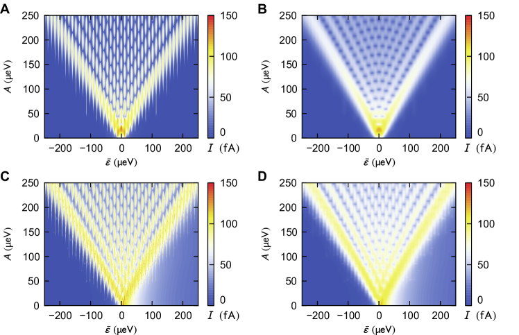
Figure 9: Eq. (2) versus full model. All data are calculated using $\Omega/2\pi=2.75\,$GHz and system parameters as listed in Table 1. (A) Analytical solution of Eq. (2). The width of the current peaks as function of $\bar{\epsilon}$ is $\delta\bar{\epsilon}=\sqrt{\Delta_{n}^{2}+\gamma^{2}}$ (containing only tunneling rates), see Eq. (2). (B) Analytical solution of Eq. (2), as in panel A, but additionally convoluted with a Gaussian profile of width $\lambda^{\star}=3.5\,\mu$eV to simulate the effect of an inhomogeneous broadening in a time ensemble measurement caused by slow charge noise. (C) Numerical solution of our full model, including electron-phonon coupling, at $T=18\,$mK (with parameters from Table 1) but using $\lambda^{\star}=0$. (D) Numerical solution of our full model as in panel C but using $\lambda^{\star}=3.5\,\mu$eV. The similarity between the analytical solutions and the low temperature result of our full model, if comparing panel A with C and panel B with D, justifies our perturbative approach to treat the electron-phonon coupling.

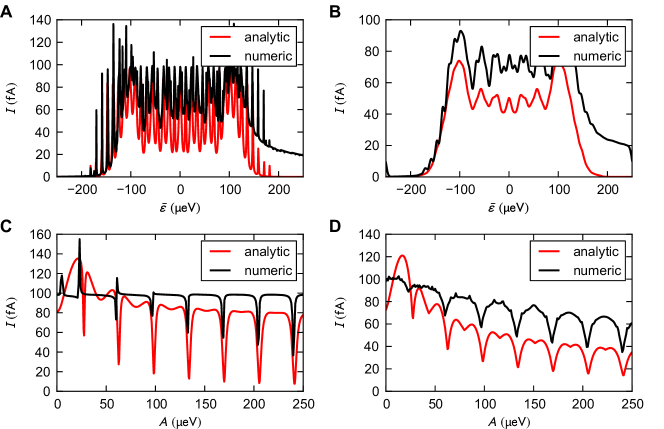
Figure 10: Eq. (2) versus full model — slices. Slices of the data in Fig. 9. Each panel compares the analytical predictions of Eq. (2) (marked as “analytic”) with those of our full model for $\alpha_{Z}=1.5\times 10^{-4}$ and at $T=18\,$mK (marked “numeric”). The modulation frequency is $\Omega/2\pi=2.75\,$GHz. (A) $I(\bar{\epsilon})$ at $A\simeq 130\,\mu$eV using $\lambda^{\star}=0$. (B) $I(\bar{\epsilon})$ at $A\simeq 130\,\mu$eV using $\lambda^{\star}=3.5\,\mu$eV. (C) $I(A)$ for $\bar{\epsilon}=0$ using $\lambda^{\star}=0$. (D) $I(A)$ for $\bar{\epsilon}=0$ using $\lambda^{\star}=3.5\,\mu$eV. For the agreement of the full model results with measured data, see Figs. 4A and B of the main text.

which provide a direct comparison between the predictions of Eq. (2) and our full model. The detailed comparison between our numerical calculations and measurements, provided in Figs. 4A and B, further demonstrates that our full model fits considerably better to our data than Eq. (2). The analytical expression in Eq. (2) only considers non-interacting electrons and, hence, fails to predict decoherence effects. A reliable physical interpretation including the observed temperature dependence (see Figs. 4C and 4 requires a detailed analysis: First, it is necessary to explicitly consider all (dot-lead and interdot) tunnel couplings and the relevant energy spectrum of the DQD. Second, interaction effects have to be included which in our case comprise: (i) Coulomb-interaction giving rise to Coulomb blockade and the coupling to charge noise; (ii) exchange interaction causing Pauli-spin blockade, hyperfine interaction causing spin-flips and the mixing between singlet and triplet states by the inhomogeneous field of the nanomagnet; (iii) electron-phonon interaction resulting in decoherence. We focus on the latter. Our master equation formalism takes into account all these effects and allows us to numerically calculate $I(\bar{\epsilon},A)$ in the range in which we take our experimental data and compute its two-dimensional discrete Fourier transformation. Finally, a Fourier transformation of our data causes cut-off effects, because both measured and calculated data span only finite ranges in $\bar{\epsilon}$ and $A$. Typical artefacts of the discrete Fourier transformation are avoided throughout our analysis as good as possible by using only data with sufficiently high resolution.

Next, we discuss the details of our data analysis: after calculating raw data resembling the measured LZSM patterns, using estimated values for $\alpha_{Z}$ and $\lambda^{\star}$ we apply the identical analysis to experimental and numerical data. Then, we compare the results and repeat calculation and analysis of the numerical data with modified $\alpha_{Z}$ and $\lambda^{\star}$ in a self-consistent way until we find best agreement with the measured data. Fig. 11

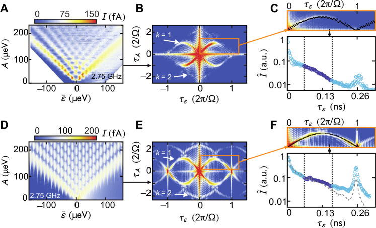
Figure 11: Data analysis based on Fourier transformation. Analysis steps on measured data (A–C) versus theory (D–F) for $T\simeq 60\,$mK and $\Omega/2\pi=2.75\,$GHz using the parameters listed in Table 1 for the numerical calculations. The numerical data in panels D–F are without the inhomogeneous broadening, i. e. $\lambda^{\star}=0$. (A and D) LZSM interference patterns $I(\bar{\epsilon},A)$. The measured data in panel A display a stronger asymmetry in $\bar{\epsilon}$ compared to the numerical data in panel D, which is discussed in Sec. A.8. (B and E) Two-dimensional Fourier transformed $\widehat{I}(\tau_{\epsilon},\tau_{A})$ of the raw data in panels A and D. Clearly visible are the principal lemon arcs for $k=1$ and those for $k=2$ in Eq. (3). Horizontal and vertical lines at $\tau_{\epsilon}=0$ and $\tau_{A}=0$, respectively, are artefacts caused by the discrete Fourier transformation. The color scales are in arbitrary units as the absolute amplitude of $\widehat{I}$ scales with the number of data points in the raw data and has no physical meaning. The higher visibility of the numerical data in panel E compared to the measured data in B is due to the negligence of the inhomogeneous broadening. (C and F) Decay of a quarter of the principal lemon arc in the range $0\lesssim\tau_{\epsilon}\lesssim 2\pi/\Omega$. The dashed line in the lowest panel is the data (open circles) multiplied by the Gaussian $\exp[-\frac{1}{2}(\lambda^{\star}\tau_{\epsilon}/\hbar)^{2}]$ using $\lambda^{\star}=3.5\,\mu$eV for direct comparison with the data in panel C. The region between the two vertical (dotted) lines is then fitted with Eq. (4) to determine $\lambda$.

demonstrates the last step of this procedure, exemplarily, for a typical set of measured data in panels A–C and the corresponding calculated data, based on our model parameters listed in Table 1, in panels D–F. The numerical data shown here neglect the inhomogeneous broadening, equivalent to using $\lambda^{\star}=0$, as this is sufficient for evaluating $\lambda$ from the numerical data. Measured and calculated data in Fig. 11, therefore, imply differences (details in figure caption); for a direct comparison including the inhomogeneous broadening in the numerical data we refer to Fig. 2 and Fig. 4. Panels A and D of Fig. 11 show the measured and calculated $I(\bar{\epsilon},A)$, respectively, panels B and E the corresponding Fourier transformed $\widehat{I}(\tau_{\epsilon},\tau_{A})$. Since the current is real-valued, the Fourier transformed pattern is point symmetric, while the approximate mirror symmetry at the $A$-axis relates the two independent branches. Therefore it is sufficient to restrict the analysis to the upper-right quarter as indicated in Figs. 11C and F. The Fourier transformed of the current along the lemon arcs $\widehat{I}(\tau_{\epsilon},\tau_{A})\big{|}_{\text{lemon}}$ incorporate a decay between two maxima at the arcs intersections at $\tau_{\epsilon}=0$ and $\tau_{\epsilon}=2\pi/\Omega$. These maxima indicate a fast intrinsic decay and are related to $\Delta_{n}^{2}$ dominating the denominator of Eq. (2) near the $n$-photon resonances. They are not a measure of the qubit decoherence. Note that finite range cut-off effects of the Fourier transformations cause the finite $\widehat{I}(\tau_{\epsilon},\tau_{A})$ along $\tau_{\epsilon}=0$ and $\tau_{A}=0$ in Figs. 11B and E, which additionally obscure the maxima in $\widehat{I}(\tau_{\epsilon},\tau_{A})\big{|}_{\text{lemon}}$. For our further analysis we therefore only consider the decay of $\widehat{I}(\tau_{\epsilon},\tau_{A})\big{|}_{\text{lemon}}$in the regions marked in Figs. 11C and F. To determine $\lambda$ the measured $\widehat{I}(\tau_{\epsilon},\tau_{A})\big{|}_{\text{lemon}}$ in Fig. 11C is fitted with Eq. (3) using $\lambda^{\star}=3.5\,\mu$eV while the calculated data in Fig. 11F are just fitted with the exponentially decaying term in Eq. (3) using $\lambda^{\star}=0$.

To accurately determine the electron-phonon coupling we consider the temperature dependence of $\lambda(\alpha_{Z},T)$ rather than relying on a single LZSM pattern at low temperature. This procedure allows us to properly separate the two main noise sources, the temperature independent charge noise giving rise to the inhomogeneous dephasing time $T_{2}^{\star}$ and the temperature dependent homogeneous broadening $\lambda$, which is directly related to $\alpha_{Z}$ and determines the qubit decoherence time $T_{2}$. (There are no indications for a temperature dependence of the charge noise for $T<1\,$K). The details of this procedure are discussed in the main article around Fig. 4. In Fig. 12A we provide additional data on the determination of the electron-phonon coupling presenting $\lambda(\alpha_{Z})$ for various temperatures. Each data point has been determined from fitting Eq. (4) to a principal lemon arc as the one in Fig. 11F calculated using the fixed $\lambda^{\star}=3.5\,\mu$eV but various values of $\alpha_{Z}$. Horizontal lines indicate $\lambda$ determined from our measured data for the same three temperatures. Assuming a temperature independent $\alpha_{Z}$ we find best agreement to our data for $\alpha_{Z}=(1.5\pm 0.2)\times 10^{-4}$ (vertical dashed line and gray region). Note that a similar information is contained in Fig. 4B. The saturation of $\lambda(T)$ for low temperatures at a value $\lambda_{\text{min}}\simeq 4\,\mu$eV is a consequence of measuring PAT current peaks which possess the intrinsic width $\sqrt{\Delta_{n}^{2}+\gamma^{2}}$ of $I(\bar{\epsilon},A)$ as a function of $\bar{\epsilon}$ expressed in Eq. (2). As is evident from Fig. 4B of the main article the lower bound $\lambda_{\text{min}}$ is also observed in our experiments. Figs. 12B and C demonstrate the robustness of our main model parameters $\alpha_{Z}$ and $\lambda^{\star}$, respectively, by varying each of the two parameters separately and comparing the decay of the principal lemon arcs.

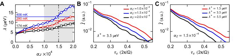
Figure 12: Analysis of the Fourier transformed — electron-phonon coupling. (A) Decay rate $\lambda(\alpha_{Z})$ for three different temperatures. The curves are numerically calculated using the fixed $\lambda^{\star}=3.5\,\mu$eV but various values of $\alpha_{Z}$. Horizontal lines indicate $\lambda$ determined from our measured data for the same three temperatures. The vertical dashed line and the gray region indicate the best fitting $\alpha_{Z}$ and its accuracy. Also compare to Fig. 4B. (B) Numerically calculated decay of the principal lemon arc for $T=295\,$mK using the fixed $\lambda^{\star}=3.5\,\mu$eV but various values of $\alpha_{Z}$ (same as those in Fig. 4B). (C) Numerically calculated decay of the principal lemon arc for $T=295\,$mK using the fixed $\alpha_{Z}=1.5\times 10^{-4}$ but various values of $\lambda^{\star}$.

A.6 Summary of data analysis

Summarizing our data analysis, we started by determining all important physical constants such as tunnel couplings and spin-flip rates based on a number of independent measurements on our double quantum dot device already tuned to the configuration used for the LZSM interferometry experiments. To determine the remaining key-parameters $\lambda^{\star}$ and $\alpha_{Z}$ we used a self-consistent approach within our model. It turned out that $\alpha_{Z}$ could be best determined from the two-dimensional Fourier transformed of LZSM interference patterns at various temperatures. In contrast, $\lambda^{\star}$, which causes a strong but temperature independent inhomogeneous broadening, could be equally well determined from the raw data. This allowed us to avoid a third fit parameter (besides $\lambda$ and a prefactor) by which we would loose precision in finding $\alpha_{Z}$. Specifically, by comparing the resulting decay rates $\lambda(T,\alpha_{Z})$ with those extracted from our measurements (see Fig. 4B), we find that in our setup decoherence can be described by a Caldeira-Leggett model with Ohmic spectral density and the dimensionless dissipation strength $\alpha_{Z}\simeq 1.5\times 10^{-4}$.

A.7 LZSM interference at various frequencies

In the main article we already demonstrate that the LZSM interference pattern depends on frequency. In Fig. 13 we extend the frequency range presenting data between $1.5\,\text{GHz}\leq\Omega/2\pi\leq 5.5\,$GHz all measured (upper line) or numerically calculated (lower line) at $T\simeq 20\,$mK.

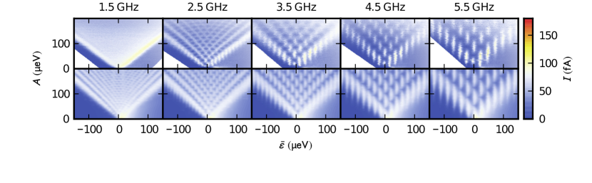
Figure 13: LZSM interference patterns for various modulation frequencies. The upper row contains measured and the lower row calculated data, both for $T\simeq 20\,$mK. Model parameters according to Table 1.

At the highest frequencies we observe clear PAT patterns as expected from Eq. (2) which distort increasingly as the frequency is lowered and neighbored PAT current peaks overlap. At $\Omega/2\pi=1.5\,$GHz all interference signatures are (almost) lost as $\hbar\Omega\simeq 6\,\mu\text{eV}$ is close to the broadening caused by the combination of our $\lambda^{\star}\simeq 3.5\,\mu$eV and $\lambda(T=20\,\text{mK})\simeq 4\,\mu$eV.

It is instructive to estimate the Landau-Zener probability $P_{\text{LZ}}=\exp(-\pi\Delta^{2}/2\hbar|v|)$ Landau1932a ; Zener1932a ; Stueckelberg1932a ; Majorana1932a for these frequencies for an intermediate amplitude, say $A=100\,\mu$eV. For $\epsilon(t)=\bar{\epsilon}+A\cos(\Omega t)$, the sweep velocity at the avoided crossing is $|v|=\Omega\sqrt{A^{2}-\bar{\epsilon}^{2}}$. Thus we find for the frequencies used in Fig. 13 and $\bar{\epsilon}=0$ Landau-Zener transition probabilities in the range $0.65\lesssim P_{\text{LZ}}\lesssim 0.89$ and $P_{\text{LZ}}\simeq 0.79$ for $\Omega/2\pi=2.75\,$GHz where we performed our temperature dependent measurements. For non-vanishing $\bar{\epsilon}$, $P_{\text{LZ}}$ is smaller, so that the average over all relevant crossings becomes of order $P_{\text{LZ}}\simeq 1/2$ which ensures good visibility. For frequencies $\Omega/2\pi\lesssim 2\,$GHz, the analytic estimate of Eq. (2) based on PAT becomes increasingly inaccurate and, consequently, our interpretation of the lemon arc decay given by Eq. (4) is not guaranteed.

A.8 Influence of dynamic nuclear polarization

The measured data, e. g. in Figs. 2A and B and in Figs. 13A–E contain two distinct features not included in our model. The first one is a pronounced asymmetry in $I(\bar{\epsilon})$ in the limit of large amplitudes, which is considerably smaller in the theoretical data, which neglect the influence of the $\text{T}_{20}$ triplet. The stronger asymmetry observed in measured data is indeed caused by the influence of the $\text{T}_{20}$ state which grows with increasing positive detuning. The effect is clearly seen in Fig. 6 and has been discussed at the end of Sec. A.1. The second feature occurs at very small amplitudes and appears as if the tip of the current triangle was shifted to slightly positive values of $\bar{\epsilon}$. It is a signature of dynamic polarization of the nuclear spins caused by the hyperfine interaction between the current carrying electrons and the nuclear spins in the DQD. At very small $A$, the rf-modulation is practically off and we simply measure the current through the DQD while sweeping $\bar{\epsilon}$ from positive towards negative values. As explained in detail in Ref. Petersen2013a , the current maximum occurs at the value of $\bar{\epsilon}$ that marks the resonance between the $T_{-}$ and the singlet state. This resonance is shifted towards positive $\epsilon$ by dynamic nuclear polarization Petersen2013a . The fact that the shift only occurs at very small $A$ indicates that the continues rf-modulation effectively prevents the polarization of nuclear spins. We therefore, do not have to include this in our model here as long as we concentrate on data with $A>20\,\mu$eV.

A.9 Temperature dependence and limitations of our model

The temperature dependence of the LZSM patterns discussed in the main article in the Figures 4C and 4 is at the heart of our model as it is used to accurately determine the electron-phonon coupling and finally the qubit coherence time $T_{2}$. So-far we have mostly concentrated on the temperature dependence of the principal lemon arc in the Fourier transformed of the LZSM patterns. Fig. 14A

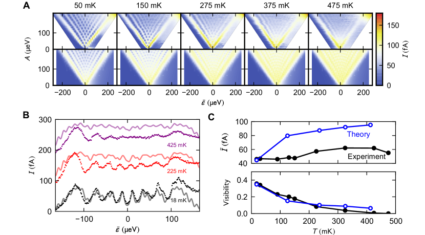
Figure 14: Temperature dependence of raw data versus model. (A) LZSM interference patterns at $\Omega/2\pi=2.75\,$GHz and various temperatures. The upper plots have been measured, the lower plots calculated using our full model with the parameters listed in Table 1. (B) Horizontal slices from plots like those in panel A at $A=130\,\mu$eV. Dots correspond to measured and lines to numerical data. (C) Average current $\bar{I}$ (upper panel) and visibility $\nu=\left(I_{\text{max}}-I_{\text{min}}\right)/\left(I_{\text{max}}+I_{\text{min}}\right)$ (lower panel), extracted from the slices presented in panel B and similar data, as function of temperature. The data points are taken in the region $-100\,\mu\text{eV}\leq\bar{\epsilon}\leq 30\,\mu\text{eV}$; this avoids the region of $\bar{\epsilon}>100\,\mu$eV where experimental data are influenced by the $\text{T}_{20}$ triplet which is neglected in our model. Black dots are measured while blue open circles are calculated.

shows LZSM patterns measured (upper line) versus calculated (lower line) at various temperatures. Fig. 14B shows horizontal slices at $A=130\,\mu$eV (dots are measured and lines present numerical data). To facilitate a quantitative comparison, we extract the visibility as well as the average current $\bar{I}$ in the region defined by $-70\,\mu\text{eV}\leq\bar{\epsilon}\leq 70\,\mu$eV and plot their temperature dependences of experimental versus numerical data in Fig. 14C. The temperature dependence of the calculated visibility resembles the measured ones. However, the measured mean current is roughly temperature independent while the predicted mean current increases with temperature. Interestingly, the decay of the principal lemon arc of the Fourier transformed is strongly related to the visibility of a LZSM pattern but not at all to the mean current. Our model, therefore, describes the decoherence of the qubit correctly while it predicts an increase of the mean current with temperature that is stronger than in the measurements. A possible explanation for this discrepancy is that in the experiment, the spectral density of the phonons is not strictly ohmic as is assumed in our model, see Sec. B.1.3. Consequently, our theoretical description may overestimate the thermal activation of some singlet-triplet transitions.

Appendix B Theoretical modelling

Our aim is to compute the LZSM interference patterns using a realistic model and to compare the results with the measured ones. Therefore we need to consider besides our DQD also its coupling to electron source and drain contacts, as well as to environmental fluctuations. In order to realistically describe our measurements, performed in the regime of Pauli-spin blockade which is partly lifted by an inhomogeneous Zeeman field of an on-chip nanomagnet, we further include spin relaxation. Our model considers all energetically accessible DQD states and all processes which play a noticeable role in our experiment. Comparing our theoretical and experimental data we find two main contributions to a noisy environment: the first is slow charge noise Fujisawa2000 ; Pioro-Ladriere2005 ; Buizert2008 ; Yacoby2013 and can be described as an inhomogeneous broadening $\lambda^{\star}$, the second is the heat bath and contributes via the electron-phonon coupling $\alpha_{Z}$. It is straightforward to independently extract other relevant system parameters from transport measurements, so that $\lambda^{\star}$ and $\alpha_{Z}$ are the only fit parameters left.

B.1 System-lead-bath model

B.1.1 Double quantum dot Hamiltonian

We include the single-particle energies $\epsilon_{L}$ and $\epsilon_{R}$ in the left / right dot, the electron-electron interactions neglecting the small exchange terms, inter-dot tunneling, and the inhomogeneous Zeeman field to obtain in second quantization the DQD Hamiltonian

$$\begin{split}H_{\text{DQD}}={}&\sum_{\ell=L,R}\epsilon_{\ell}n_{\ell}+U\sum_{\ell=L,R}n_{\ell}(n_{\ell}-1)+U^{\prime}n_{L}n_{R}\\ &+\frac{\Delta}{2\sqrt{2}}\sum_{m=\uparrow,\downarrow}(c_{Lm}^{\dagger}c_{Rm}+c_{Rm}^{\dagger}c_{Lm})\\ &+\frac{g\mu_{\text{B}}}{2}\sum_{\ell=L,R}(c_{\ell,{\uparrow}}^{\dagger},c_{\ell,{\downarrow}}^{\dagger})(\vec{B}_{\ell}\cdot\vec{\sigma})(c_{\ell,{\uparrow}},c_{\ell,{\downarrow}})^{T},\end{split}$$ (6)

where $n_{\ell}=\sum_{m=\uparrow\downarrow}c_{\ell m}^{\dagger}c_{\ell m}$ is the occupation of dot $\ell=L,R$ expressed with the usual fermionic creation and annihilation operators. The largest energy scales are the intra- and inter-dot Coulomb interactions $U$ and $U^{\prime}$, which define the diabatic basis states of our charge qubit with energies $\epsilon(\text{S}_{20})=2\epsilon_{L}+U$ and $\epsilon(\text{S}_{11})=\epsilon_{L}+\epsilon_{R}+U^{\prime}$ and their mutual detuning $\bar{\epsilon}\equiv\epsilon(\text{S}_{20})-\epsilon(\text{S}_{11})=\epsilon_{L}-\epsilon_{R}+U-U^{\prime}$. The fourth term describes tunneling between the dots with the matrix element $\Delta$ defined such that it equals the energy splitting of the charge qubit formed by the singlets. The final Zeeman term affects the triplet states and, because of the inhomogeneous field contribution of our on-chip magnet, also mixes singlets with triplets. This mixing enables transitions between singlet and triplet states and may be rather sensitive to thermal exitations Ribeiro2013b . If a source-drain voltage is applied across the DQD, it causes a finite average current. Notice that also the hyperfine interaction causes electron spin-flips, which we capture by a phenomenological spin-flip rate $\gamma_{\sigma}$.

B.1.2 Dot-lead Hamiltonians

To model the single electron tunneling current through the DQD we have to consider its interaction with the two-dimensional leads. Starting from the configuration (1,0), the right quantum dot is loaded via the tunneling process $(0,1)\to(1,1)$ from the source contact, i. e. the right lead. The latter is modeled as non-interacting electrons with the Hamiltonian $H_{\text{lead}}=\sum_{q,m={\uparrow}{\downarrow}}E_{q}c_{q,m}^{\dagger}c_{q,m}$ while the dot-lead coupling terms reads

$$H_{\text{dot--lead}}=\sum_{q,m=\uparrow\downarrow}V_{q}(c_{R,m}^{\dagger}c_{q,m}+c_{q,m}^{\dagger}c_{R,m}).$$ (7)

Here, the lead-to-dot tunnel probability into a specific electronic dot state with energy $E_{q}$ is proportional to the equilibrium population $\langle c_{q,m}^{\dagger}c_{q,m}\rangle=f(E_{q}-\mu_{R})$ with the source contact characterized by the Fermi function $f(E-\mu_{R})=[e^{(E-\mu_{R})/k_{\text{B}}T}+1]^{-1}$ at temperature $T$ and chemical potential $\mu_{R}$. For simplicity, we assume within a wide-band approximation that the spectral density of the source contact is energy independent and find the tunnel coupling $\Gamma_{R}(E)=2\pi\sum_{q}|V_{q}|^{2}\delta(E-E_{q})\equiv\Gamma_{R}$ between the right dot ond the source contact. The tunnel coupling between the left dot and the drain contact (left lead) is defined accordingly. Since the coupling term $V_{q}$ is sample dependent and not a priory known (it can be tuned by gate voltages), we have determined the effective dot-lead tunnel couplings, $\Gamma_{L}$ and $\Gamma_{R}$, experimentally by independent dc-measurements without applying an rf-field. Note that the decay rate used in the main article is $\Gamma_{\text{out}}=\Gamma_{L}$, while the initialization rate $\Gamma_{\text{in}}$ combines $\Gamma_{R}$ with the singlet-triplet couplings in the last term of the Hamiltonian in Eq. (6).

B.1.3 System-bath Hamiltonian

A central aim of our study is to investigate our two-electron charge qubit and its decoherence, caused by the coupling to a dissipating environment, which is encoded in the LZSM pattern and its visibility. The details in the experimentally observed fading of the LZSM pattern with increasing temperature reveal two main environmental influences captured by $\lambda^{\star}$ and $\alpha_{Z}$: the first one is an inhomogeneous broadening most likely caused by slow charge noise; the second influence is the phonon bath Schinner2009 ; Granger2012a which yields quantum dissipation and direct decoherence. Another possible decoherence source is the coupling to circuit noise which is important for typically impedance matched superconducting qubits Makhlin2001b . In our case, however, we expect this external noise source to be of minor relevance owing to a strong impedance mismatch.

For the inhomogeneous broadening, we assume that it stems from practically temperature independent slow fluctuations of the local potential that remain constant during the typical dwell time of an electron in the DQD. Therefore we can capture these fluctuations by convoluting their amplitude distribution with $I(\bar{\epsilon},A)$.

For describing decoherence that stems from the interaction between the DQD and bulk phonons, we employ a system-bath approach in the spirit of the Caldeira-Leggett model for the dissipative two-level system. This means that we couple the DQD to an ensemble of harmonic oscillators described by the Hamiltonian $H_{\text{bath}}=\sum_{\nu}\hbar\omega_{\nu}a_{\nu}^{\dagger}a_{\nu}$, where $a_{\nu}^{\dagger}$ and $a_{\nu}$ are the usual bosonic creation and annihilation operators for a phonon of frequency $\omega_{\nu}$. The position operators of the bath oscillators couple to the occupation difference between the left and the right dot, $Z=n_{L}-n_{R}$, according to

$$H_{\text{dot--bath}}=\sum_{\nu}\lambda_{\nu}(a_{\nu}^{\dagger}+a_{\nu})Z\,.$$ (8)

This electron-phonon coupling Hamiltonian describes the interaction of the DQD with environmental degrees of freedom. Its immediate effect is that fluctuations in the environment detune the electronic states which, in turn, results in a randomization of the relative phase in a superposition of states with distinct charge distribution, in particular of the singlets representing our qubit. The latter is therefore subject to decoherence. An important characteristic of a dissipating bath is its spectral density $J(\omega)=\pi\sum_{\nu}|\lambda_{\nu}|^{2}\delta(\omega-\omega_{\nu})$. As for the leads, we assume also for the phonon bath a continuum limit and replace $J(\omega)$ by the Ohmic spectral density $J(\omega)=\pi\alpha_{Z}\omega/2$. The dimensionless electron-phonon coupling strength $\alpha_{Z}$ reflects the dissipation strength, which together with the temperature parametrizes the decoherence due to the phonon bath. The Ohmic spectral density represents the natural choice which we have tested by performing additional numerical calculations using super-Ohmic spectral densities $J(\omega)\propto\omega^{s+1}$ with $s>0$, which however failed to reproduce the experimentally observed fading of the LZSM pattern with increasing temperature. A possible explanation for the good agreement of our data with an Ohmic spectral phonon density is the quasi one-dimensional character of the electron-phonon interaction in our DQD sample: decoherence is mainly caused by the one-dimensional subset of phonons with wavevector parallel to the line connecting the two quantum dots. For one-dimensional problems, the Ohmic spectral density of the electron-phonon coupling is microscopically justified Weiss1999a .

While $\alpha_{Z}$ couples to the diagonal of the Hamiltonian in Eq. (6), one may in addition consider the off-diagonal coupling term, namely the coupling between phonons and the interdot tunnel barrier. For this purpose, one introduces a further dot–bath Hamiltonian like that in in Eq. (8) but with $Z$ replaced by $X=\sum_{m=\uparrow,\downarrow}(c_{Lm}^{\dagger}c_{Rm}+c_{Rm}^{\dagger}c_{Lm})$ and the coupling strength denoted by $\alpha_{X}$. Unlike the bath-coupling via $Z$, the bath now entails a fluctuating tunnel matrix element. Therefore, $\alpha_{X}$, much more than $\alpha_{Z}$, drives transitions between the quantum dots by phonon emission or absorption. Analyzing this effect, we found a significant asymmetry of the current as function of the detuning, which is in contrast to our experimental results. The quantitative comparison with our measurements revealed that $\alpha_{X}$ is roughly two orders of magnitude smaller than $\alpha_{Z}$. In summary, $\alpha_{X}$ is of minor relevance for the qubit decoherence and need not be taken into account.

B.2 Charge qubit formed by two-electron singlet states

The simplest implementation of a DQD charge qubit is a single electron that tunnels between two dots. Nevertheless, here we consider the more complex case of two electrons charging a DQD. For the sake of applications, the two-electron state has the important advantage that it allows one to utilize both, charge and spin degrees of freedoms in a single DQD. This opens up a number of interesting possibilities, such as using either the singlet-singlet or one of the singlet-triplet transitions to define a qubit or even to combine both by subsequently sweeping through adjacent avoided crossings. Furthermore, the two-electron configuration constitutes the simplest possible many-body problem which yields a theoretically more interesting system compared to a single electron. Here, we focus on the two singlet states

$$|\text{S}_{20}\rangle={} c_{L{\uparrow}}^{\dagger}c_{L{\downarrow}}^{\dagger}|0\rangle,$$ (9)

$$|\text{S}_{11}\rangle={} \frac{1}{\sqrt{2}}(c_{L{\uparrow}}^{\dagger}c_{R{\downarrow}}^{\dagger}+c_{L{\downarrow}}^{\dagger}c_{R{\uparrow}}^{\dagger})|0\rangle,$$ (10)

which span the Hilbert space of our qubit, where $|0\rangle$ is the uncharged state of the DQD. In this singlet subspace, the double dot Hamiltonian defined in Eq. (6) reads

$$H_{\text{qubit}}=\frac{\Delta}{2}\sigma_{x}+\frac{\epsilon}{2}\sigma_{z}-\frac{\epsilon}{2}\mathbbm{1},$$ (11)

(which is equivalent to Eq. (1)) with the unity matrix $\mathbbm{1}$. The electron-phonon coupling operator defined in Eq. (8) then contains $Z=\sigma_{z}$. This leads us to the well-known spin-boson model with energy splitting $E=\sqrt{\Delta^{2}+\epsilon^{2}}$ and dissipation strength $\alpha=\alpha_{Z}$ defined in the usual way Leggett1987a .

B.2.1 Qubit decoherence

The qubit reaches thermal equilibrium within the energy relaxation time $T_{1}$ while in the limit of weak dissipation, $\alpha_{z}k_{\text{B}}T\ll E$, its pseudo-spin performs coherent oscillations which decay exponentially within the coherence time $T_{2}$ (assuming that the electron-phonon coupling is the main decoherence mechanism). From a corresponding Bloch-Redfield master equation (see below), both decay times can be determined Hanggi1990a ; Makhlin2001b :

$$T_{1}^{-1}={} \frac{\pi\alpha_{Z}}{\hbar}\frac{\Delta^{2}}{E}\coth\Big{(}\frac{E}{2k_{\text{B}}T}\Big{)},$$ (12)

$$T_{2}^{-1}={} \frac{1}{2}T_{1}^{-1}+\frac{\pi\alpha_{Z}}{\hbar}\frac{2k_{\text{B}}T\epsilon^{2}}{E^{2}}.$$ (13)

In the high-temperature limit, $k_{\text{B}}T\gg E$, the decoherence rate is proportional to the temperature: $T_{2}^{-1}=\pi\alpha_{Z}[1+\epsilon^{2}/E^{2}]k_{\text{B}}T/\hbar$. In the low-temperature limit, $k_{\text{B}}T\ll E$, quantum fluctuations take over and the coherence time becomes temperature independent, $T_{2}=2T_{1}=(2\hbar/\pi\alpha_{Z})(E/\Delta^{2})$. For temperatures $T\gtrsim\hbar\Delta/k_{B}$, decoherence is weakest near $\epsilon=0$, while for $|\epsilon|\gg\Delta$, the dephasing time decays proportional to $1/\epsilon$. Thus, at these relatively high temperatures $\epsilon=0$ defines a sweet point for quantum operations provided that the environment predominantly couples via the occupation operator $Z=\sigma_{z}$, i. e., for $\alpha_{X}\ll\alpha_{Z}$ as assumed in Eqs. (12) and (13). In the opposite limit $\alpha_{X}\gg\alpha_{Z}$ a likewise spin-boson model would result in Eqs. (12) and (13), but with the parameters $\Delta$ and $\epsilon$ interchanged and $\alpha_{Z}$ replaced by $\alpha_{X}$.

Eq. (13) overestimates the coherence time of our specific charge qubit based on two-electron states in a DQD as it uses a two-level approximation which neglects spin flips and the triplet states. In order to determine the qubit dephasing beyond the two-level approximation, we follow the lines of Ref. Fonseca2004a and employ the Bloch-Redfield formalism (see Sec. B.3). In contrast to our transport calculations, we here disregard the dot-lead couplings and consider a qubit in a closed DQD configuration. We aim at obtaining the Liouville operator for the DQD coupled to the phonon bath and further including spin flips. Decoherence is manifest in the transient decay of off-diagonal density matrix elements. The coherence time, $T_{2}$, is straightforwardly found by computing the eigenvalues of the Liouville operator. To compute $T_{2}$ we, hence, evaluate the equation of motion of the total density operator beyond the rotating-wave approximation (see below and Eq. (15)), albeit using a time-independent Hamiltonian. One finds a pair of eigenvalues with imaginary parts close to $\pm E$ which correspond to coherent qubit oscillations. Their real parts are equal and can be identified as $T_{2}^{-1}$.

In Fig. 15 we compare the coherence time $T_{2}$ as a function of temperature calculated analytically with Eq. (13) (weakly dissipative spin-boson model, two-level approximation), on the one hand, and the numerical result of the complete problem, on the other hand. This reveals that the two-level approximation overestimates $T_{2}$ by about 15% since it cannot capture incoherent singlet-triplet transitions induced by spin-flips and dephasing.

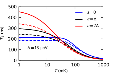
Figure 15: Temperature dependence of the qubit coherence. Decoherence time $T_{2}$ for our $\text{S}_{20}$-$\text{S}_{11}$ qubit for various values of the detuning $\epsilon$. The solid lines visualize Eq. (13) considering the electron-phonon coupling in a two-level model, while the dashed lines are computed numerically for the full DQD Hamiltonian which, in addition, takes the triplet states and e. g. spin-flips into account.

For the temperature range of of experiment, $T\gtrsim 20$ mK, the sweet point at $\epsilon=0$ is most favorable and predicts $T_{2}$ times up to 200 ns which, however, become significantly smaller with increasing temperature and bias. In the sub milli-Kelvin regime, we observe the opposite. There the strongly biased situation corresponds to pure phase noise for which the spin-boson model predicts $T_{2}\propto 1/k_{B}T$. This leaves some room for speculating about a coherence gain by further cooling. With such extrapolation, however, we leave the range in which our experiments justify the ohmic bath model.

B.2.2 Advantage of a steady state experiment

Previous measurements of the dephasing time Nowack2007a ; Bluhm2011 relied on an explicit time-trace of Ramsey fringes, where for each instance of time a probability was reconstructed from a large number of destructive measurements of a transient. Such an averaging technique requires repeated identical preparation. Owing to the inhomogeneous broadening caused by slow noise, the time-trace of the averaged probability oscillations obtained typically decays on a much smaller time scale $T_{2}^{*}$, hence $T_{2}$ is not directly accessible. Our data, by contrast, are measured in the stationary state of a much simpler experiment. In the resulting LZSM pattern, inhomegeneous broadening and decoherence are manifest in separate ways. Crucially, as a consequence, $T_{2}^{\star}$ and $T_{2}$ can be distinguished in the analysis described in Sec. A and the main article.

B.3 Bloch-Redfield-Floquet theory

We aim at computing the time-averaged steady-state current through our strongly driven DQD including an appreciable number of levels coupled to the various environments, namely (i) the leads, (ii) slow charge noise, and (iii) the heat bath. Moreover, dealing with two-electron states we have to include spin flips which allow transitions between the triplet and singlet sub-spaces and resolve spin blockade. Our experimental results are consistent with the assumption that all these incoherent processes occur on time scales much larger than those of the coherent DQD dynamics, as is indicated by the following experimental observations: (i) the coupling to the leads and the spin relaxation rate ultimately determine the maximal current that we may observe. The latter is significantly smaller than the inter-dot tunnel frequency multiplied by the elementary charge, i. e., $\Gamma_{L/R}\ll\Delta$. (ii) Charge noise is rather slow as compared to all these tunneling processes. Therefore we can treat it as disorder that is constant during the dwell time of an electron in the DQD. In other words, it leads to an inhomogeneous broadening that does not affect the decoherence dynamics of the electrons. (iii) The appearance of an interference pattern indicates that the inter-dot tunneling must be predominantly coherent which excludes strong coupling to a heat bath. This is confirmed by our finding that the dimensionless dissipation strength is several orders of magnitude below the crossover to the so-called incoherent tunneling regime Hanggi1990a . We can not a-priory exclude stronger coupling to a small number of individual (tunneling) defects, but the fact that we did not find any memory effects makes such a strong coupling scenario unlikely.

B.3.1 Floquet ansatz

To cope with the complex problem outlined above we use a reduced density matrix approach with the Floquet states of the driven system in the absence of the environments as basis states. These basis states already incorporate the rf-modulation and, therefore, allow us to apply a rotating-wave approximation, conveniently resulting in a time independent Liouville equation. This perturbative approach is reliable under the assumption of only weakly coupled environments. It has been applied in the past to both rf-driven dissipative quantum systems Kohler1997a and rf-driven quantum transport Kohler2005a .

Floquet theory exploits the fact that a periodically time-dependent Schrödinger equation of the type $i\hbar\partial|\psi\rangle/\partial t=H_{\text{DQD}}(t)|\psi\rangle$ possesses a complete set of solutions of the form $|\psi(t)\rangle=e^{-i\omega t}|\phi(t)\rangle$, where $\hbar\omega$ is called quasienergy. The Floquet state $|\phi(t)\rangle=|\phi(t+2\pi/\Omega)\rangle\equiv\sum_{k}e^{-ik\Omega t}|\phi_{k}\rangle$ is characterized by shareing the time-periodicity of the Hamiltonian. Therefore, it can be represented as Fourier series which, importantly, allows an efficient numerical treatment. In analogy to quasimomenta in Bloch theory employed for spatially periodic potentials, in Floquet theory the quasienergies can be divided into Brillouin zones of equivalent states. Thus, it is sufficient to solve the eigenvalue problem within one Brillouin zone, e. g. for $-\Omega/2\leq\omega<\Omega/2$. By inserting the Floquet ansatz into the Schrödinger equation, we obtain the eigenvalue equation

$$\Big{(}H_{\text{DQD}}(t)-i\hbar\frac{\partial}{\partial t}\Big{)}|\phi(t)\rangle=\hbar\omega|\phi(t)\rangle$$ (14)

from which we compute a complete set of Floquet states, $\{|\phi_{n}\rangle\}$, and the corresponding quasienergies $\hbar\omega_{n}$ .

B.3.2 Bloch-Redfield theory

An established technique for studying a quantum system in weak contact with an environment is Bloch-Redfield theory. It is based on a treatment of the system-environment coupling operator $V$ within second-order perturbation theory by which one finds for the total density operator the equation of motion Blum1996a

$$\dot{R}=-\frac{i}{\hbar}[H_{\text{DQD}}(t)+H_{\text{env}},R]-\frac{1}{\hbar^{2}}\int_{0}^{\infty}d\tau[V,[V(t-\tau,t),R]]\,.$$ (15)

The particular form of the coupling operator in the interaction picture, $V(t-\tau,t)=U_{\text{DQD}}^{\dagger}(t-\tau,t)VU_{\text{DQD}}(t-\tau,t)$, stems from the explicit time-dependence of the central quantum system. By tracing out the environmental degrees of freedom, one obtains an equation of motion for the reduced density operator of the system, $\rho$. This step requires one to specify the state of the environment. Here, we assume that it is in the grand canonical state $\rho_{\text{env}}^{\text{(eq)}}$ and that it is uncorrelated with the system, such that the total density operator factorizes into a system and an environment part, $R\simeq\rho\otimes\rho_{\text{env}}^{\text{(eq)}}$. Under this condition the decomposition into the Floquet basis provides a master equation of the form $\dot{\rho}=-i(\omega_{n}-\omega_{m})\rho_{mn}+\sum_{n^{\prime}m^{\prime}}L_{nm,n^{\prime}m^{\prime}}\rho_{n^{\prime}m^{\prime}}$, where the Bloch-Redfield tensor $L_{nm,n^{\prime}m^{\prime}}$ follows in a straightforward way from Eq. (15). In the last step we assume that all matrix elements $\rho_{nm}$ evolve much slower than the rf-field, which allows us to replace the Bloch-Redfield tensor by its time average. In this way we obtain a time-independent master equation describing the time evolution of the population of the (time dependent) Floquet states.

We are exclusively interested in the steady state of this master equation, which for weak dissipation eventually becomes diagonal in the Floquet basis. Exploiting this knowledge, we set the off-diagonal matrix elements to zero and arrive at a master equation of the form

$$\dot{\rho}_{nn}=\sum_{n^{\prime}}\Big{(}W_{n\leftarrow n^{\prime}}\rho_{n^{\prime}n^{\prime}}-W_{n^{\prime}\leftarrow n}\rho_{nn}\Big{)}\,,$$ (16)

where $\rho_{nn}$ are the populations of the Floquet states. In the following we present the results for the transition rates $W_{n\leftarrow n^{\prime}}$ which are evaluated as sketched above.

B.3.3 Coupling between the double quantum dot and the leads

To calculate the tunnel coupling between the right lead and the right quantum dot, we evaluate the coefficients of the master Eq. (16) by replacing $V$ in Eq. (15) with the tunnel coupling between the right dot and the right lead given by Eq. (7). After some algebra, we arrive at the transitions rates

$$\begin{split}W_{n\leftarrow n^{\prime}}^{\text{leads}}={}&\frac{\Gamma_{R}}{\hbar}\sum_{k}\Big{|}\sum_{k^{\prime}}\langle\phi_{n,k^{\prime}+k}|c_{R}^{\dagger}|\phi_{n^{\prime},k^{\prime}}\rangle\Big{|}^{2}\\ &\qquad\times f(\omega_{n}-\omega_{n^{\prime}}+k\Omega-\mu_{R})\\ &+\frac{\Gamma_{R}}{\hbar}\sum_{k}\Big{|}\sum_{k^{\prime}}\langle\phi_{n,k^{\prime}+k}|c_{R}|\phi_{n^{\prime},k^{\prime}}\rangle\Big{|}^{2}\\ &\qquad\times(1-f(\omega_{n}-\omega_{n^{\prime}}+k\Omega-\mu_{R})),\end{split}$$ (17)

where the first term describes tunneling from the right lead to the right dot, while the second term refers to the opposite process. The corresponding Liouvillian for coupling to the left lead is obtained in the same way with the accordingly modified dot-lead Hamiltonian. Owing to charge conservation, the time-averaged currents are the same at all interfaces. Here we evaluate it at the right dot-lead barrier and obtain it as the difference between the terms that describe in Eq. (17) tunneling from the lead to the dot and those describing the opposite process:

$$\begin{split}J_{n\leftarrow n^{\prime}}={}&-\frac{\Gamma_{R}}{\hbar}\sum_{k}\Big{|}\sum_{k^{\prime}}\langle\phi_{n,k^{\prime}+k}|c_{R}^{\dagger}|\phi_{n^{\prime},k^{\prime}}\rangle\Big{|}^{2}\\ &\qquad\times f(\omega_{n}-\omega_{n^{\prime}}+k\Omega-\mu_{R})\\ &+\frac{\Gamma_{R}}{\hbar}\sum_{k}\Big{|}\sum_{k^{\prime}}\langle\phi_{n,k^{\prime}+k}|c_{R}|\phi_{n^{\prime},k^{\prime}}\rangle\Big{|}^{2}\\ &\qquad\times(1-f(\omega_{n}-\omega_{n^{\prime}}+k\Omega-\mu_{R})),\end{split}$$ (18)

where $J_{n\leftarrow n}=0$ due to vanishing matrix elements. Note that this expression can also be derived in a more formal way by introducing a counting variable for the lead electrons before tracing them out and, thus, it does not rely on any specific interpretation of the tunneling terms.

B.3.4 Coupling between the qubit states and the heat bath

A Liouvillian that describes the influence of the dissipating environment on the DQD is derived by the same procedure, but using for $V$ the electron-phonon Hamiltonian Eq. (7). We obtain

$$\begin{split}W_{n\leftarrow n^{\prime}}^{\text{decoherence}}=&2\sum_{k}\Big{|}\sum_{k^{\prime}}\langle\phi_{n,k^{\prime}+k}|Z|\phi_{n^{\prime},k^{\prime}}\rangle\Big{|}^{2}\\ &\times N(\omega_{n}-\omega_{n}^{\prime}+k\Omega),\end{split}$$ (19)

where $N(\omega)=J(\omega)n_{\text{th}}(\omega)$ with the bosonic thermal occupation number $n_{\text{th}}(\omega)=[e^{\hbar\omega/k_{\text{B}}T}-1]^{-1}$. In order to arrive at this convenient form, we have defined $J(-\omega)=-J(\omega)$, while the Bose function was extended by analytic continuation.

As already mentioned, a coherent tunnel process between the charge configurations (1,1) and (2,0) requires that the spin configuration of both states is equal, and in our case this includes only the singlet states $\text{S}_{11}$ and $\text{S}_{20}$. The reason is, that the triplet $\text{T}_{20}$ is too high in energy owing to the large intradot exchange interaction. In turn, a direct transition of the triplet states with (1,1) charge configuration to $\text{S}_{20}$ is inhibited. As a consequence the transport process comes to a standstill until a transition to the $\text{S}_{11}$ singlet occurs. In our setup, this spin blockade is resolved by two mechanisms. First, the Zeeman field of the nanomagnet close to the DQD possesses an inhomogeneity by which singlets and triplets mix. They form narrow avoided crossings at which spin blockade is resolved and a current peak emerges. This effect is fully coherent and contained in our DQD Hamiltonian, Eq. (6). Second, spin flips are induced by the hyperfine interaction with nuclear spins in the GaAs matrix, which we treat as incoherent relaxation. Therefore, thermal motion of the nuclear spins coupled via the hyperfine interaction represent a further dissipative environment. Our LZSM measurements do not provide clear experimental hints on memory effects (besides for very small modulation amplitudes $A$, where we find indications for dynamic nuclear spin polarization, see Sec. A.8) or a significant temperature dependence of the spin flip rate (within the probed temperature range). This allows us to avoid the theoretical difficulties of choosing a particular microscopic model and to capture spin flips by a Lindblad form with a rate $\gamma_{\sigma}$. Therefore, we add to the master equation the Liouvillean $L[\rho]=\frac{1}{2}\gamma_{\sigma}\sum_{\ell,m={\uparrow}{\downarrow}}(2S_{\ell,m}\rho S_{\ell,m}^{\dagger}-S_{\ell,m}^{\dagger}S_{\ell,m}\rho-\rho S_{\ell,m}^{\dagger}S_{\ell,m})$ with the spin flip operator $S_{\ell,m}=c_{\ell,\bar{m}}^{\dagger}c_{\ell,m}$ for an electron on dot $\ell$, where $m={\uparrow},{\downarrow}$ and $\bar{m}\neq m$. Decomposition into Floquet states followed by rotating-wave approximation yields the rate

$$W_{n\leftarrow n^{\prime}}^{\text{spinflip}}=\gamma_{\sigma}\sum_{m={\uparrow}{\downarrow}}\sum_{k}\Big{|}\sum_{k^{\prime}}\langle\phi_{n,k^{\prime}+k}|S_{L,m}|\phi_{n^{\prime},k^{\prime}}\rangle\Big{|}^{2}\,.$$ (20)

DQD parameter	value in $\mu$eV		determined by
bias voltage $V$	1000		externally applied voltage
intra dot Coulomb energy $U$	$3500\pm 350$		charging diagram
inter dot Coulomb interaction $U^{\prime}$	$820\pm 80$		charging diagram
inter-dot tunnel coupling $\Delta$	$13\pm 1$		spin funnel, see Fig. 7C
source-dot tunnel rate $\Gamma_{R}$	0.1		estimated from current, of minor relevance
dot-drain tunnel rate $\Gamma_{L}$	$2\times 10^{-3}{}^{\dagger}$		from current without spin blockade
spin relaxation $\gamma_{\sigma}$	$10^{-3}$		from current with spin blockade
$\mathrm{T}_{\pm}-\text{S}_{11}$ splitting	$0.12^{\ddagger}$		Landau-Zener transition, see Fig. 7A
external parameters	value in $\mu$eV		determined by
photon energy $\hbar\Omega$	$6.2/11.4/18.7$		at modulation frequency of $1.5/2.75/4.5$ GHz
mean Zeeman splitting $g\mu_{\text{B}}B$	4.2		$g\mu_{\text{B}}B_{\text{ext}}$; $|g|=0.36$ and $B_{\text{ext}}=200\,$mT
thermal energy $k_{B}T$	1.7 – 40		cryostat and electron temperature
environmental influences	value		determined by
inhomogeneous broadening $\lambda^{\star}$	$3.5\pm 0.5\,\mu$eV		from broadening in $I(\bar{\epsilon})$ peaks
Caldeira-Leggett parameter $\alpha_{Z}$	$(1.5\pm 0.5)\times 10^{-4}$		decay of lemon arcs, temperature dependence
Caldeira-Leggett parameter $\alpha_{X}$	$<5\times 10^{-6}$		asymmetry of LZSM pattern

Table 1: Parameters used for the numerical calculations. ^† The data of Fig. 2 and Fig. 13 were measured with a slightly smaller dot-drain rate and, accordingly, the numerical data were computed with $\Gamma_{R}=1.2\times 10^{-3}\,\mu$eV. ^‡ Note that the S-T splittings are reduced compared to $g\mu_{\text{B}}\Delta B_{x,z}$ according to the weight of $\text{S}_{20}$ in the singlet state. In our case we have $g\mu_{\text{B}}\Delta B_{x}\simeq 0.2\,\mu$eV which reduces to the $\mathrm{T}_{\pm}-\text{S}_{11}$ splitting of $0.12\,\mu$eV.

In our numerical approach to the steady-state average current, we first compute the Floquet states which allows us to evaluate the transition probabilities:

$$W_{n\leftarrow n^{\prime}}=W_{n\leftarrow n^{\prime}}^{\text{leads}}+W_{n\leftarrow n^{\prime}}^{\text{decoherence}}+W_{n\leftarrow n^{\prime}}^{\text{spinflip}}\,,$$ (21)

so that we obtain a specific expression for the master equation Eq. (16). The steady-state solution of this master equation, $\rho_{nn}^{(\infty)}$, follows straigtforwardly from the condition $\dot{\rho}_{nn}^{(\infty)}=0=\sum_{n^{\prime}}(W_{n\leftarrow n^{\prime}}\rho_{n^{\prime}n^{\prime}}^{(\infty)}-W_{n^{\prime}\leftarrow n}\rho_{nn}^{(\infty)})$ together with the trace condition $\sum_{n}\rho_{nn}^{(\infty)}=1$. Finally we arrive at the dc current $I=\sum_{nn^{\prime}}J_{n\leftarrow n^{\prime}}\rho_{n^{\prime}n^{\prime}}^{(\infty)}$.

Appendix C System parameters

Table 1 summarizes the most important parameters which characterize our DQD, the two-electron qubit and its coupling to the environment and which we used in our numerical calculations. For applying the scattering formula Eq. (2), we identified the initialization rate $\Gamma_{\text{in}}$ for the process $(1,0)\to\text{S}_{11}$ with the spin relaxation rate $\gamma_{\sigma}$, while the decay $(2,0)\to(1,0)$ occurs at dot-draim rate so that $\Gamma_{\text{out}}=\Gamma_{L}$.

References

- (1) L. D. Landau, Phys. Z. Sowjetunion 2, 46 (1932).
- (2) C. Zener, Proc. R. Soc. London, Ser. A 137, 696 (1932).
- (3) E. C. G. Stueckelberg, Helv. Phys. Acta 5, 369 (1932).
- (4) E. Majorana, Nuovo Cimento 9, 43 (1932).
- (5) W. D. Oliver, Y. Yu, J. C. Lee, K. K. Berggren, L. S. Levitov, and T. P. Orlando, Science 310, 1653 (2005).
- (6) M. Sillanpää, T. Lehtinen, A. Paila, Y. Makhlin, and P. Hakonen, Phys. Rev. Lett. 96, 187002 (2006).
- (7) C. M. Wilson, T. Duty, F. Persson, M. Sandberg, G. Johansson, and P. Delsing, Phys. Rev. Lett. 98, 257003 (2007).
- (8) D. M. Berns, M. S. Rudner, S. O. Valenzuela, K. K. Berggren, W. D. Oliver, L. S. Levitov, and T. P. Orlando, Nature (London) 455, 51 (2008).
- (9) S. N. Shevchenko, S. Ashhab, and F. Nori, Phys. Rep. 492, 1 (2010).
- (10) P. Huang, J. Zhou, F. Fang, X. Kong, X. Xu, C. Ju, and J. Du, Phys. Rev. X 1, 011003 (2011).
- (11) J. Stehlik, Y. Dovzhenko, J. R. Petta, J. R. Johansson, F. Nori, H. Lu, and A. C. Gossard, Phys. Rev. B 86, 121303(R) (2012).
- (12) E. Dupont-Ferrier, B. Roche, B. Voisin, X. Jehl, R. Wacquez, M. Vinet, M. Sanquer, and S. De Franceschi, Phys. Rev. Lett. 110, 136802 (2013).
- (13) C. Gang, L. Hai-Ou, T. Tao, W. Li, Z. Cheng, X. Ming, G. Guang-Can, J. Hong-Wen, and G. Guo-Ping, Nature Commun. 4, 1401 (2013), 10.1038/ncomms2412.
- (14) P. Nalbach, J. Knörzer, and S. Ludwig, Phys. Rev. B 87, 165425 (2013).
- (15) H. Ribeiro, G. Burkard, J. R. Petta, H. Lu, and A. C. Gossard, Phys. Rev. Lett. 110, 086804 (2013).
- (16) M. Ciorga, A. S. Sachrajda, P. Hawrylak, C. Gould, P. Zawadzki, S. Jullian, Y. Feng, and Z. Wasilewski, Phys. Rev. B 61, R16315 (2000).
- (17) K. Ono, D. G. Austing, Y. Tokura, and S. Tarucha, Science 297, 1313 (2002).
- (18) G. Petersen, E. A. Hoffmann, D. Schuh, W. Wegscheider, G. Giedke, and S. Ludwig, Phys. Rev. Lett. 110, 177602 (2013).
- (19) H. Bluhm, S. Foletti, I. Neder, M. Rudner, D. Mahalu, V. Umansky, and A. Yacoby, Nature Phys. 7, 109 (2011).
- (20) Y. Kayanuma, Phys. Rev. A 50, 843 (1994).
- (21) M. Strass, P. Hänggi, and S. Kohler, Phys. Rev. Lett. 95, 130601 (2005).
- (22) G. Granger et al., Nature Phys. 8, 522 (2012).
- (23) P. Hänggi, P. Talkner, and M. Borkovec, Rev. Mod. Phys. 62, 251 (1990).
- (24) Y. Makhlin, G. Schön, and A. Shnirman, Rev. Mod. Phys. 73, 357 (2001).
- (25) T. Fujisawa and Y. Hirayama, Applied Physics Letters 77, 543 (2000).
- (26) M. Pioro-Ladrière, J. H. Davies, A. R. Long, A. S. Sachrajda, L. Gaudreau, P. Zawadzki, J. Lapointe, J. Gupta, Z. Wasilewski, and S. Studenikin, Phys. Rev. B 72, 115331 (2005).
- (27) C. Buizert, F. H. L. Koppens, M. Pioro-Ladrière, H.-P. Tranitz, I. T. Vink, S. Tarucha, W. Wegscheider, and L. M. K. Vandersypen, Phys. Rev. Lett. 101, 226603 (2008).
- (28) O. E. Dial, M. D. Shulman, S. P. Harvey, H. Bluhm, V. Umansky, and A. Yacoby, Phys. Rev. Lett. 110, 146804 (2013).
- (29) M. S. Rudner, A. V. Shytov, L. S. Levitov, D. M. Berns, W. D. Oliver, S. O. Valenzuela, and T. P. Orlando, Phys. Rev. Lett. 101, 190502 (2008).
- (30) U. Weiss and M. Wollensak, Phys. Rev. Lett. 62, 1663 (1989).
- (31) K. M. Fonseca-Romero, S. Kohler, and P. Hänggi, Chem. Phys. 296, 307 (2004).
- (32) T. Hayashi, T. Fujisawa, H. D. Cheong, Y. H. Jeong, and Y. Hirayama, Phys. Rev. Lett. 91, 226804 (2003).
- (33) K. D. Petersson, J. R. Petta, H. Lu, and A. C. Gossard, Phys. Rev. Lett. 105, 246804 (2010).
- (34) S. Kohler, J. Lehmann, and P. Hänggi, Phys. Rep. 406, 379 (2005).
- (35) M. Field, C. G. Smith, M. Pepper, D. A. Ritchie, J. E. F. Frost, G. A. C. Jones, and D. G. Hasko, Phys. Rev. Lett. 70, 1311 (1993).
- (36) D. Taubert, D. Schuh, W. Wegscheider, and S. Ludwig, Review of Scientific Instruments 82, 123905 (2011).
- (37) J. R. Petta, A. C. Johnson, J. M. Taylor, E. A. Laird, A. Yacoby, M. D. Lukin, C. M. Marcus, M. P. Hanson, and A. C. Gossard, Science 309, 2180–2184 (2005).
- (38) H. Ribeiro, J. R. Petta, and G. Burkard, Phys. Rev. B 87, 235318 (2013).
- (39) G. J. Schinner, H. P. Tranitz, W. Wegscheider, J. P. Kotthaus, and S. Ludwig, Phys. Rev. Lett. 102, 186801 (2009).
- (40) U. Weiss, Quantum Dissipative Systems, 2nd ed. (World Scientific, Singapore, 1998).
- (41) A. J. Leggett, S. Chakravarty, A. T. Dorsey, M. P. A. Fisher, A. Garg, and W. Zwerger, Rev. Mod. Phys. 59, 1 (1987).
- (42) K. C. Nowack, F. H. L. Koppens, Yu. V. Nazarov, and L. M. K. Vandersypen, Science 318, 1430 (2007).
- (43) S. Kohler, T. Dittrich, and P. Hänggi, Phys. Rev. E 55, 300 (1997).
- (44) K. Blum, Density Matrix Theory and Applications, 2nd ed. (Springer, New York, 1996).