Generic Image Classification Approaches Excel on Face Recognition

Abstract

The main finding of this work is that the standard image classification pipeline, which consists of dictionary learning, feature encoding, spatial pyramid pooling and linear classification, outperforms all state-of-the-art face recognition methods on the tested benchmark datasets (we have tested on AR, Extended Yale B, the challenging FERET, and LFW-a datasets). This surprising and prominent result suggests that those advances in generic image classification can be directly applied to improve face recognition systems. In other words, face recognition may not need to be viewed as a separate object classification problem.

While recently a large body of residual based face recognition methods focus on developing complex dictionary learning algorithms, in this work we show that a dictionary of randomly extracted patches (even from non-face images) can achieve very promising results using the image classification pipeline. That means, the choice of dictionary learning methods may not be important. Instead, we find that learning multiple dictionaries using different low-level image features often improve the final classification accuracy. Our proposed face recognition approach offers the best reported results on the widely-used face recognition benchmark datasets. In particular, on the challenging FERET and LFW-a datasets, we improve the best reported accuracies in the literature by about 20% and 30% respectively.

1 Introduction

In recent years, researchers have spent significant effort on appearance based face recognition. In particular, (sparse) representation based face classification has shown success in the literature [28, 34]. Given a test face image, the classification rule is based on the minimum representation error over a set of training facial images. In this category, one of the well-known methods might be the sparse representation based classifier (SRC) [28]. SRC linearly represents a probe image by all the training images under the sparsity constraint/regularisation using the $L_{1}$ norm. The success of SRC has induced a few sparse representation based algorithms [33, 7, 31, 8]. Competitive results have been observed using non-sparse $L_{2}$ norm regularised representations [34, 21, 24]. The main advantage of these approaches is its computational efficiency due to the closed-form solution. Zhang et al. argued that it is the collaborative representation but not the $L_{1}$ sparsity that boosts the face recognition performance [34]. Their method is dubbed as Collaborative Representation Classification (CRC).

Instead of focusing on the encoding strategy and directly using the training samples as the dictionary, another research topic is to learn a dictionary using improved variants of sparse coding. Yang et al. [32] proposed a dictionary learning method using the Fisher discrimination criterion. Dictionary learning was formulated as an extended K-SVD problem in [35] and [14], where the classification error was taken into the objective function. To alleviate the effect of image noise contamination, low-rank minimisation of dictionary was utilised with the help of class discrimination [19] or structural incoherence of basis [4].

Almost all of these methods use holistic images. Local feature descriptors such as histograms of Local Binary Patterns (LBP) [2], Gabor wavelets [17] have been proven to improve the robustness of face recognition systems. A heuristic method is the modular approach, which first partitions the entire facial image into several blocks and then classification is made independently on each of these local blocks. The intermediate results on local patches are finally aggregated, e.g., by distance-based evidence fusion (DEF) [21] or majority voting [28]. Zhu et al. [36] proposed a multi-scale patch based method, which fused the results of patches of all scales with the scale weights learned by regularized boosting.

All the aforementioned representation based methods make classification decisions based on the representation errors/residuals. In contrast, the encoded coefficients themselves have not been fully exploited for face recognition. This is very different from the simplest, standard pipeline of generic image classification, such as the Bag-of-Features (BoF) model. [5]. The BoF model [26, 5] is generally composed of dictionary learning on local features (either raw pixels or dense SIFT features), feature encoding and spatial pyramid pooling. The locally encoded and spatially aggregated feature representation, coupled with an efficient linear classifier (e.g., linear support vector machines (SVM)), has been the standard approach to generic image classification, including fine-grained image classification, and object detection.

A striking and surprising result of our work here is that the simple, standard generic image classification approach using unsupervised feature learning outperforms the best face recognition methods. This finding suggests that face recognition may not need to be tackled as a separate problem—generic object recognition approaches work extremely well on face recognition. A bold suggestion is that for the problem of face recognition, it may be better to shift the research focus from the recognition component to the pre-processing component, e.g., facial feature detection and alignment, which often benefits the subsequent recogniser.

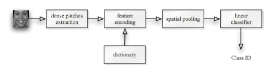
Figure 1: An illustration of the standard image classification pipeline.

Recently, Coates et al. showed that for image classification, a very simple module combination (dictionary of patches learned using K-means or even random selection with a simplified non-linear encoder) can achieve state-of-the-art image classification performances on benchmark datasets such as CIFAR and CalTech101 [5, 6]. Our baseline face recognition system follows this simple pipeline of [30, 5], which is illustrated in Fig. 1. Namely, we solve the face recognition problem using the pipeline of dictionary learning, feature encoding and spatial pooling followed by linear classification. We also thoroughly evaluate the impact of each stage in the pipeline on the final face recognition performance. Some interesting results are found, which provide insightful suggestions to the face recognition community.

In summary, our main contributions are as follows.

• We show that, given the raw-pixel face images, simple feature learning coupled with a highly efficient linear classifier can achieve state-of-the-art face recognition performances on widely-used face benchmark datasets. We thus suggest that face recognition can be tackled as an instance of generic image classification, advances of which can help boost the face recognition research.

• The generic image classification pipeline (including dictionary learning, encoding and pooling) is thoroughly evaluated in the scenario of face recognition. We show that dictionary learning is less important than that of feature encoding. This is consistent with the observation in [5]. In particular, we show that a dictionary using random patches, without learning involved, can work very well.

  Another interesting finding is that, using this recognition pipeline, a dictionary learned using non-face patches can also achieve excellent results. That is, a face image patch can be represented by using non-face image patches. In contrast, all the previous representation based face recognition methods (SRC [28], CRC [34], LRC [21] etc.) are restricted to use facial training images to form the dictionary.

• Composed of inner product and simple non-linear activation function, the soft threshold encoding performs close to (however much faster than) sparse coding. Actually in some situations (e.g., with large class number and less training data) soft threshold achieves even better results than sparse coding. This deviates the results found on the CIFAR and CalTech101 image classification [5].

• Last, we show that a simple fusion of the learned features using raw-pixel intensity and LBP further improves the classification performance over features learned using raw-pixel or LBP alone.

Next, before we present our main results, we briefly introduce the image classification pipeline using unsupervised feature learning.

2 Image classification and feature learning

Image classification, which classifies an image into one or a few categories, has been one of the most fundamental problems in computer vision. Possibly due to the special characteristics of face images and historical reasons, face recognition has so far been considered as a different task from generic image classification. However, in essence, face recognition is a sub-category or fine-grained object classification problem. Indeed, for the first time, we show that generic object recognition methods work extremely well on face recognition.

The generic image classification pipeline (shown in Fig. 1) has achieved state-of-the-art performances [26, 5]. Low-level features on local patches are usually densely extracted and pre-processed (normalisation and whitening) in the first step. It has been shown that the pre-processing steps can have considerable influence on the final classification performance [6]. With the extracted local patches, an over-complete dictionary is formed by using unsupervised learning, e.g, K-means, K-SVD, or sparse coding [30]. The image patches are then encoded with the learned dictionary, e.g., using the hard vector quantisation, variants of sparse encoding [30, 26] or soft threshold [5]. To encode the spatial information as well as reduce the dimension of the generated features, the encoded features are pooled over the pre-defined spatial cells either using average pooling or max-pooling, results of which are concatenated to form the final representation of an image. Last, a linear classifier is trained with the learned image features.

2.1 Unsupervised dictionary learning

In this work, we use the following methods to construct the dictionary ${\mathbf{D}}\in\mathbf{R}^{d\times m}$. Here $m$ is the number of atoms, and $d$ is the input dimension. We have chosen these methods mainly due to their computational scalability and efficiency. Suppose that we have extracted $N$ small local patches $\{{\mathbf{x}}_{i}\}$ from the training data.

• Random selection: The dictionary ${\mathbf{D}}$ is directly formed by the $m$ patches randomly selected from $\{{\mathbf{x}}_{i}\}$. No learning is involved.

• K-means clustering: We apply K-means clustering on local patches $\{{\mathbf{x}}_{i}\}$ and fill the columns of ${\mathbf{D}}$ with the $m$ cluster centres.

• Sparse coding: Sparse coding forms an over-complete dictionary by minimising the reconstruction error with the $L_{1}$ sparsity constraint. The objective function can be written as [5]:

  $$\min_{D,{\mathbf{f}}_{i}} \sum_{i}\|{\mathbf{D}}{\mathbf{f}}_{i}-{\mathbf{x}}_{i}\|^{2}_{2}+\lambda\|{\mathbf{f}}_{i}\|_{1}$$

  $${\,\,\mathrm{s.t.\,\,}} \|{\mathbf{D}}_{j}\|_{2}=1,\quad\forall j.$$ (1)

  Here ${\mathbf{D}}_{j}$ is the $j$th dictionary atom ($j$th column of the matrix ${\mathbf{D}}$).

• K-SVD: As a generalization of K-means, K-SVD shares a similar objective function as sparse coding [1]. It has been used for generating dictionary for residual based face recognition [35, 14].

2.2 Feature encoding

Once the dictionary is obtained, local patches are then fed into the feature encoder to generate a set of codes $\{{\mathbf{f}}_{i}\}$. We use the following encoding methods.

• Sparse coding: With ${\mathbf{D}}$ fixed in (1), ${\mathbf{f}}_{i}$ can be obtained by solving the LASSO problem.

• Locality-constrained linear coding: Compared with sparse encoding, LLC [26] is more efficient, which solves for the code of a sample by a constrained least square problem with its $K$ nearest neighbours.

• Ridge regression: If one replaces the $L_{1}$-norm regularisation with the $L_{2}$-norm regularisation, one has the ridge regression problem, which admits a closed-form solution. We can generate the code directly by the ridge regression problem.

  In [34], the authors reformulate the $L_{1}$ optimisation of SRC into a $L_{2}$ ridge regression problem for face recognition.

• Soft threshold: With a fixed threshold $\alpha$, this simple feed-forward non-linear encoder writes [5]:

  $${\mathbf{f}}_{j}({\mathbf{x}})= \max\big{\{}0,{\mathbf{D}}_{j}^{\!\top}{\mathbf{x}}-\alpha\big{\}},$$ (2)

  $${\mathbf{f}}_{j+m}({\mathbf{x}})= \max\big{\{}0,-{\mathbf{D}}_{j}^{\!\top}{\mathbf{x}}-\alpha\big{\}}.$$ (3)

  Here ${\mathbf{f}}_{j}$ is the $j$th entry of the encoded feature vector ${\mathbf{f}}$.

• K-means triangle: As a ‘softer’ extension of the hard-assignment coding, with the $m$ centroids $\{{\mathbf{c}}_{j}\}$ learned by K-means, K-means triangle encode ${\mathbf{x}}$ as:

  $${\mathbf{f}}_{j}({\mathbf{x}})=\max\big{\{}0,\mu({\mathbf{z}})-{\mathbf{z}}_{j}\big{\}},$$ (4)

  where ${\mathbf{z}}_{j}=\|{\mathbf{x}}-{\mathbf{c}}_{j}\|$ and $\mu({\mathbf{z}})$ is the mean of ${\mathbf{z}}$.

  We can also use this encoding method by replacing $\{{\mathbf{c}}_{j}\}$ with the bases generated by other dictionary learning methods other than K-means. See [6] for details.

2.3 Linear classifiers

A simple ridge regression based classifier is used in [11]. We use the same linear classifier for its computational efficiency. One can of course use linear SVM such as LIBLINEAR [9]. However, for large-scale high-dimensional data, LIBLINEAR is still slow. The ridge regression classifier has a closed-form solution, which is very fast. Despite its simplicity, the classification performance of this ridge regression approach is on par with linear SVM [11].

Let ${\mathbf{X}}\in\mathbf{R}^{n\times d}$ be the training data of $n$ samples of dimension $d$ and ${\mathbf{Y}}\in\{0,1\}^{n\times c}$ the label matrix: ${\mathbf{Y}}_{ij}=1$ if data point $i$ belongs to class $j$ of total $c$ classes and 0 otherwise. Unlike SVM, this classifier generates the classifier matrix with a closed-form solution ${\mathbf{W}}=({\mathbf{X}}^{{\!\top}}{\mathbf{X}}+\delta{\mathbf{I}})^{-1}{\mathbf{X}}^{{\!\top}}{\mathbf{Y}}$, where ${\mathbf{I}}$ is the identity matrix. Then an image ${\mathbf{z}}$ is classified by the maximum of ${\mathbf{W}}^{{\!\top}}{\mathbf{z}}$. Another benefit of this classifier is that, compared to the one-versus-all SVM, it only needs to compute ${\mathbf{W}}$ once. When the number of classes is large, training of multiple one-versus-all classifiers also creates the problem of imbalanced data (the number of positive data is much smaller than that of negative data). This ridge regression classifier does not have this problem. In practice the dimension $d$ could be over hundreds of thousands when with several pooling pyramid levels.

We thus compute the matrix ${\mathbf{W}}$ by its equivalent ${\mathbf{W}}={\mathbf{X}}^{{\!\top}}({\mathbf{X}}{\mathbf{X}}^{{\!\top}}+\delta{\mathbf{I}})^{-1}{\mathbf{Y}}$, where it only needs to invert much smaller $n\times n$ matrix.

3 Evaluation of the pipeline for face recognition

In this section, we test the feasibility and performance of classifying face images exactly same as in classifying natural images, and try to discover what the most important component is. Thorough cross evaluations of the components in the image classification pipeline are conducted on face recognition.

Following [5], local patches are extracted on data with patch size of $6\times 6$ pixels and a stride of $1$ pixel, followed by contrast normalization and ZCA whitening [13]. It has been proven that dense feature extraction and the pre-processing step are critical for achieving better performance.

Unless otherwise specified, we generate the dictionary from 50,000 randomly extracted patches on the training data. In all the experiments except those in section 3.1, the threshold $\alpha$ in soft threshold and the regularization parameter $\lambda$ in sparse coding are set to 0.25 and 1, respectively. As a default setup in the evaluation, the final features are formed by max pooling over 3 pyramid levels.

We mainly conduct evaluations on the datasets of AR and Extended Yale B, and LFW. The datasets description can be found in section 4. In this section we use 13 and 32 training samples each class for AR and Extended Yale B, respectively. The rest are used for testing. For LFW-a, 5 samples are randomly selected for training and another 2 samples for testing in each class.

3.1 Dictionary learning and feature encoding

First, we evaluate the impact of the dictionary size on face recognition performance. Fig. 2 shows the results of our method with the dictionary size varying from 100 to 2,000. It is not surprising to see that the accuracy is consistently improved as the dictionary size increases. Coates et al. [5] observed that a large dictionary often leads to improved classification accuracy, especially when one has a limited number of labelled training data for training the final classifier. This is the case for face recognition. In the following experiments we set the dictionary size to 1,600.

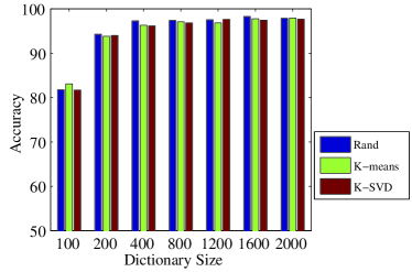
Figure 2: Impact of the size of the dictionary (obtained by random selection, K-means and K-SVD) on the recognition accuracy (%). The AR dataset is used. Here the encoding strategy is soft thresholding for efficiency.

Next, we then examine the importance of dictionary learning and feature encoding methods for face recognition. Four methods of dictionary construction: randomly selected patches (uniform sampling), K-means, K-SVD [1], sparse coding [30]; and five encoding algorithms: sparse coding, LLC [26], $L_{2}$ ridge regression, soft threshold, K-means triangle [6] are evaluated. We set the maximum number of iterations for K-SVD to 30, and the number of nearest neighbours $K=5$ for LLC. We conduct K-SVD with sparsity level $T=\{3,5,10,15,30\}$, sparse coding with $\lambda=\{0.25,0.5,1.0,1.5\}$, LLC with the regularization parameter $\delta=\{0.001,0.01,0.1,1\}$, soft threshold with $\alpha=\{0.1,0.25,0.5,0.75,0.1\}$. By maximizing over these parameters, best cross validation results with each combination of the dictionary learning and encoding methods are reported. Table 1 and Table 2 list the recognition results on the AR and LFW datasets, respectively.

Encoder	ST	SC	LLC	RR	KT	VQ
Random	97.8	98.8	98.2	95.7	97.5	94.5
K-means	97.8	98.5	97.2	95.6	97.1	92.9
K-SVD	98.2	98.6	98.4	96.1	97.8	95.1
SC	98.1	98.4	98.9	97.7	98.5	94.3

Table 1: Accuracies (%) with various dictionary learning methods (shown in the first column) and encoding methods (shown in the first row) on AR. ‘SC’, ‘LLC’, ‘RR’, ‘ST’, ‘KT’ and ‘VQ’ represent ‘Sparse Coding’, ‘Locality-constrained Linear Coding’, ‘Ridge Regression’, ‘Soft Threshold’, ‘K-means Triangle’ and hard ‘Vector Quantization’, respectively. The results at each column are similar, which shows that dictionary learning methods do not have a significant impact on the final performance.

Encoder	ST	SC	LLC	RR	KT	VQ
Random	$75.4\pm 1.6$	$76.4\pm 1.8$	$76.5\pm 0.5$	$68.2\pm 3.6$	$78.0\pm 1.2$	$62.5\pm 2.1$
K-means	$75.4\pm 1.6$	$77.2\pm 2.3$	$72.9\pm 2.2$	$64.6\pm 2.1$	$77.9\pm 0.9$	$60.6\pm 2.1$
K-SVD	$75.4\pm 1.6$	$77.6\pm 2.8$	$75.1\pm 0.8$	$69.1\pm 1.4$	$79.0\pm 1.2$	$61.6\pm 1.1$
SC	$74.7\pm 1.9$	$74.3\pm 3.7$	$75.7\pm 3.1$	$72.6\pm 1.1$	$80.0\pm 2.3$	$60.3\pm 0.4$

Table 2: Accuracies (%) with various dictionary learning methods (shown in the first column) and encoding methods (shown in the first row) on LFW. Results are based on 5 independent runs.

As we can see, with an encoder fixed (such as soft threshold or sparse coding), different dictionary learning methods lead to similar classification results. In other words, dictionary learning is less critical in terms of the final performance. As observed in [5], for face recognition we see similar observations: simple algorithms like K-means can work as well as sparse coding and K-SVD in most cases. In general, Vector Quantization (VQ) as in the traditional bag-of-visual-words model, performs worse than other encoding methods because VQ may have lost much useful information due to the aggressive hard-assignment coding.

In [5], the authors show that a dictionary of randomly selected patches usually performs slightly worse on CIFAR and CalTech101. While for face recognition, we see that even with a dictionary of randomly selected patches, the performance is as good as other dictionary learning methods such as sparse coding when the size of the dictionary is large (1,600 is sufficient in our experiments).

This is in contrast to the representation error based methods, where it is important to design an effective dictionary (in order to reconstruct the test image well), e.g., by sample variations [7, 8], discriminative learning [32] or low-rank minimization [19, 4].

Among the encoding approaches, sparse coding achieves the best results on the AR dataset, which marginally outperforms other encoding methods with most dictionary training methods. The simple and computationally efficient encoder ‘soft threshold’ and ‘K-means Triangle’ also stably offer promising results, which is much better than ridge regression and VQ on this dataset. On the relatively challenging dataset LFW, the simple algorithm K-means triangle works even better than all other methods with any dictionary learning methods. Note that K-means triangle does not have a parameter to tune.

Consistent with the finding for generic image classification [5], we can see from this experiment that the choice of dictionary learning methods is less important than that of feature encoder in the face image classification pipeline. Random patches combined with a simple encoder, which introduces non-linearity, can work very well. In general, the conclusion is that most non-linear encoding methods yield promising results for face recognition. Here we show some learned bases generated by different dictionary learning methods in Fig. 3.

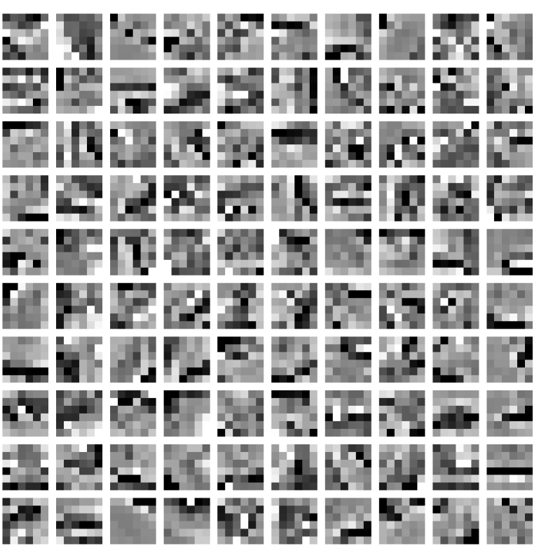
(a) Randomly selected patches

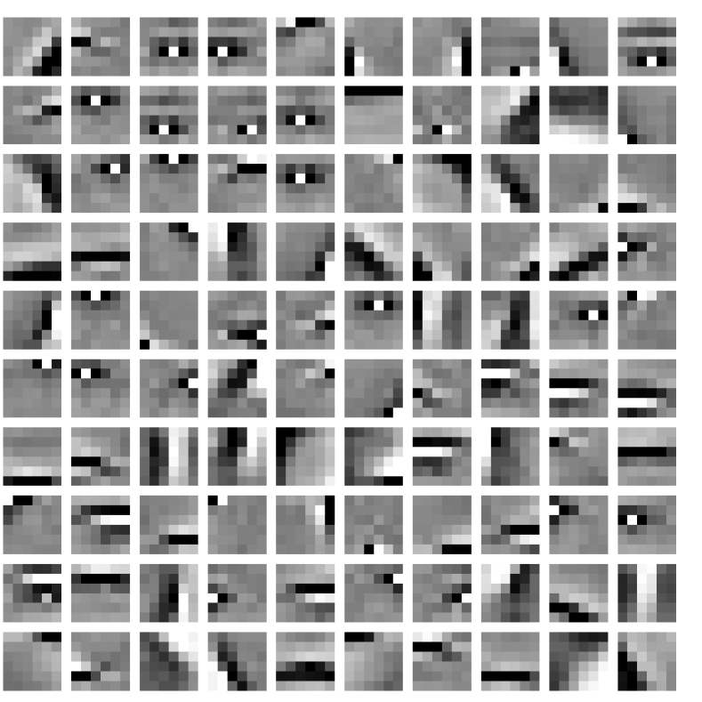
(b) K-means

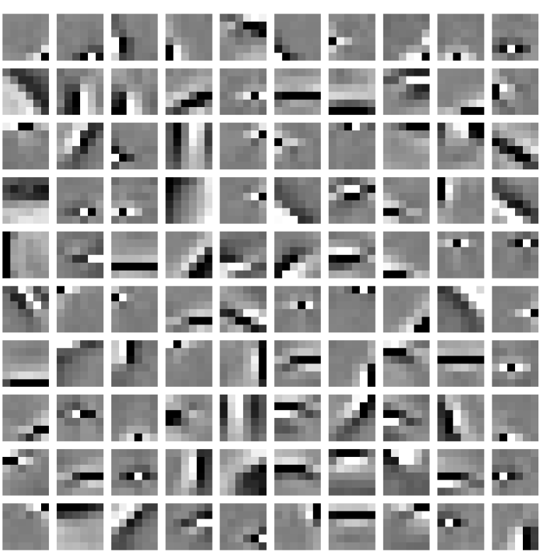
(c) K-SVD

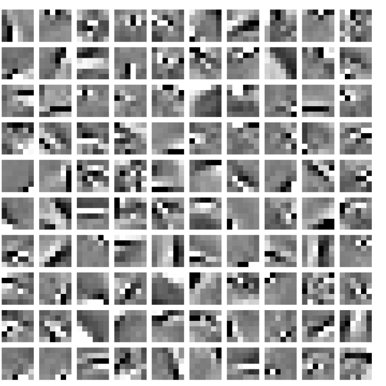
(d) Sparse coding

Figure 3: Visualisation of some generated dictionary bases by a few different dictionary construction methods. The bases generated by different methods appear similarly.

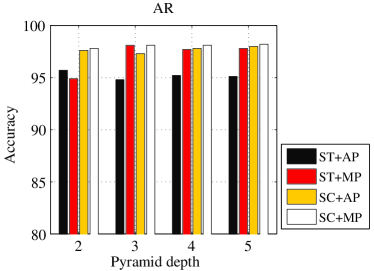
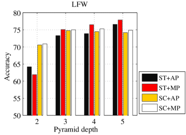
Figure 4: Accuracies (%) with different number of spatial pyramid levels on the AR and LFW-a datasets. ‘ST’, ‘SC’, ‘AP’ and ‘MP’ represent ‘Soft Threshold’, ‘Sparse Coding’, ‘Average Pooling’ and ‘Max Pooling’, respectively.

3.2 Spatial pyramid pooling

In this subsection, we evaluate the two popular pooling method: sum/average pooling and max pooling with varying pyramid levels. With pyramid pooling, the encoded features for all local patches are pooled over each grid of all spatial pyramid levels [18]. We set the first a few levels to have {$1\times 1$, $2\times 2$, $4\times 4$, $6\times 6$, $8\times 8$} equal-sized rectangular pooling grids. The pooled features at each level are concatenated to form the final feature vectors.

Fig. 4 shows the results on AR and LFW-a [27]. The first observation is that spatial pyramid pooling is important for the final classification performance.

We can clearly see that, max pooling is almost always better than average pooling except for soft threshold with fewer pyramid levels. This is consistent with recent results for image classification [3]. From Fig. 4, we also see that soft threshold encoding achieves increasing accuracies as pyramid depth increases, especially on the challenging LFW-a dataset [27]. As for sparse coding, the performance does not improve significantly when the pyramid depth is already more than three. With max pooling and three or more pyramid levels, soft threshold obtains close results with sparse coding on AR and even better results on LFW-a. Note that soft threshold encoding is simple and computationally much more efficient than sparse coding.

Test	Dictionary
	AR	ExYale B	CIFAR-10
AR (ST)	97.8	97.6	97.5
AR (SC)	98.2	98.2	97.8
ExYale B (ST)	99.8	99.8	99.8
ExYale B (SC)	98.0	98.7	98.3

Table 3: Recognition accuracies (%) on AR and Extended Yale B (ExYale B) of our method using different datasets (listed on the second row) for dictionary generation.

3.3 Representing faces using a dictionary learned from non-face image patches

In this subsection, we test whether the training data for dictionary learning is critical. We generate the dictionary using both the training data from the testbed dataset and on additional datasets. For example, we test on the AR dataset with dictionary trained on AR or Extended Yale B. From Table 3, we can see that on par results are obtained by training on the same dataset from the test data or a different one.

In addition, we further evaluate the dictionary generated on datasets of non-face images. Here we use a subset of CIFAR-10, which includes 10,000 natural images. It is surprising that learning a dictionary using the dataset of non-face images also works very well. That is, a face image can be recognised using a representation learned from non-face images. This is impossible for the representation error based methods like SRC. This property is desirable because one can obtain a dictionary that is as large as needed even when lacking of training face data.

The reason why learning face representations using non-face data works so well might be as follows. We have used the single-layer unsupervised feature learning to generate the dictionary. It is well known that single-layer dictionary learning such as sparse coding mainly learns image filters that resemble Gabor-like filters. Small patches extracted from either face images or non-face images would both learn Gabor-like filters. However, for multiple-layer hierarchical feature learning, one expects that using object-specific training data might learn more meaningful high-level features.

4 Experimental results

In this section, we compare our methods with several state-of-the-art algorithms on four benchmark face recognition databases. These compared algorithms include SRC, CRC, robust sparse coding (RSC [33]), the Fisher discrimination criterion based dictionary learning method FDDL [32], patched based MSPCRC [36] and PNN [16]. For these methods we use the codes and recommended settings provided by the authors.

From the pilot experiments in the last section, we know that the important factors for the final face recognition performance are: the image patch size and stride step, encoding methods, and the pooling strategy. We now report results using various encoding methods; and the patch size and stride step are set to be small ($6\times 6$ pixels and the stride step is 1 pixel in all of the experiments). All the results of our method in this section are based on max-pooling with 5 pyramid pooling levels. We set the dictionary size to 1,600 in all experiments, which are randomly sampled from 50,000 small patches. Therefore, no learning is involved in dictionary learning for our approach.

4.1 Extended Yale B

The Extended Yale B dataset [10] consists of 2414 frontal face images from 38 subjects under various lighting conditions. The images are cropped and normalized to $192\times 168$ pixels [31]. To increase the difficulty, in each class we randomly choose only 10 sample for training and another 5 samples for testing. All the images are finally resized to $32\times 32$. We run experiments on 5 independent data splits and report the average results in Table 4.

It is clear that our method with soft threshold encoding achieves the highest average accuracy of 97.3%, which is better than MSPCRC. In contrast, the best result among all other methods is only 92.6% (obtained by FDDL). Our method with sparse coding does not perform as well as soft threshold on this dataset. We have not carefully tuned the regularization parameter in sparse coding. Careful tuning of this parameter might improve the performance of sparse coding.

We also list in Table 5 the recent published results of several sate-of-the-art methods on this dataset. It is clear that our method outperforms all other methods with 99.8% accuracy. To our knowledge, ours is the best published result with the same settings on the Extended Yale B dataset.

Method	CRC	SRC	RSC	FDDL	MSPCRC	Ours (ST)	Ours (SC)
Accuracy	$91.9\pm 0.8$	$89.0\pm 1.2$	$89.7\pm 0.5$	$92.6\pm 1.3$	$97.1\pm 1.5$	${\bf 97.3\pm 1.3}$	$91.0\pm 2.1$

Table 4: Recognition accuracies (%) and their standard deviations on the Extended Yale B dataset with dimension $32\times 32$. Results are based on 5 independent runs.

Method	Training size	Dimension	Accuracy
DLRD [19]	32	$24\times 21$	98.2
FDDL [32]	20	$54\times 48$	91.9
LC-KSVD [14]	32	$24\times 21$	96.7
LSC [25]	32	$104\times 91$	99.4
Low-Rank [4]	32	100 (PCA)	97.0
RSC [33]	32	300 (PCA)	99.4
Ours	32	$32\times 32$	99.8

Table 5: Published results (%) in the literature on the Extended Yale B dataset. Number of training images per class are shown in the second column and the rest are for test. Soft threshold encoding is used for our method.

Method	CRC	SRC	RSC	FDDL	MSPCRC	Ours (ST)	Ours (SC)
$32\times 32$	$59.4\pm 1.1$	$75.5\pm 1.5$	$73.0\pm 2.2$	$79.4\pm 1.4$	$41.0\pm 1.6$	${\bf 94.3\pm 0.5}$	${\bf 95.9\pm 1.0}$
$64\times 64$	$54.0\pm 0.8$	$73.6\pm 1.5$	$73.0\pm 2.2$	$79.5\pm 1.8$	$41.9\pm 2.2$	${\bf 97.0\pm 0.7}$	${\bf 98.8\pm 0.5}$

Table 6: Recognition accuracies (%) and their standard deviations on FERET with dimension $32\times 32$ and $64\times 64$. Results are based on 5 independent runs.

4.2 FERET

The FERET dataset [23] is another widely-used standard face recognition benchmark set provided by DARPA. We use a subset of FERET which includes 200 subjects. Each individual contains 7 samples, exhibiting facial expressions, illumination changes and up to 25 degrees of pose variations. It is composed of the images whose names are marked with ‘ba’, ‘bj’, ‘bk’, ‘be’, ‘bf’, ‘bd’ and ‘bg’. The images are cropped and resized to $80\times 80$ [29]. We randomly choose 5 samples in each class for training and the rest 2 samples for testing. The mean results of 5 independent runs with down-sampled $32\times 32$ and $64\times 64$ images are reported in Table 6.

Different from Extended Yale B, FERET has a large number of classes and exhibits pose variations. On this dataset, we can see that our methods perform significantly better than previously reported results. Almost all other methods do not achieve satisfactory results.

Our method with sparse coding obtains an average accuracy of 98.8% with image dimension $64\times 64$ pixels, which outperforms the previous best result of FDDL [32] by a large margin of about 20%. Note that our method is based on randomly extracted patches, while the dictionary of FDDL is trained by a very expensive process. MSPCRC does not perform well on this dataset.

4.3 AR

Method	CRC	SRC	RSC	FDDL	Ours (ST)	Ours (SC)
AR (Occlusion)	84.5	86.5	88.5	83.5	97.8	98.2
AR (Clean)	88.4	92.9	92.3	85.9	98.4	98.9

Table 7: Recognition accuracies (%) on the AR dataset with dimension of $32\times 32$ pixels. ST and SC are our methods with soft threshold and sparse coding, respectively.

Method	Situation	Dimension	Accuracy
LSC [25]	Clean	$116\times 84$	90.0
FDDL [32]	Clean	$60\times 43$	92.0
DLRD [19]	Clean	$27\times 20$	95.0
RSC [33]	Clean	300 (PCA)	96.0
Ours	Clean	$64\times 64$	99.1
L2 [24]	Occlusion	$168\times 120$	95.9
ESRC [7]	Occlusion	$168\times 120$	97.4
SSRC [8]	Occlusion	$168\times 120$	98.6
Ours	Occlusion	$64\times 64$	99.2

Table 8: Published results (%) on AR dataset in two situations. Sparse coding is used for our method.

The AR dataset [20] consists of over 4000 facial images from 126 subjects (70 men and 56 women). For each subject 26 facial images were taken in two separate sessions. The images exhibit a number of variations including various facial expressions (neutral, smile, anger, and scream), illuminations (left light on, right light on and all side lights on), and occlusion by sunglasses and scarves. Of the 126 subjects available 100 have been selected in our experiments (50 males and 50 females). All the images are finally resized to $32\times 32$ pixels.

We first test on the AR dataset in two situations: with occlusions and without occlusions. For the first situation, the 13 samples in the first session are used for training and the other 13 images in the second session for test. For the second ‘clean’ situation, the 7 samples in each session with only illumination and expression changes are used. From Table 7, we can see that both of our two methods with soft threshold encoding and sparse coding encoding obtain the best results on these two situations. The previous best results of other methods in the occlusion and clean situation are obtained by RSC and SRC, which are worse than our method with sparse coding by 9.8% and 10%, respectively.

We also list in Table 8 the recent published results of several sate-of-the-art methods on AR. It is clear that our method achieves the highest accuracies (99.1% and 99.2% for the clean and occlusion situation, respectively). To the best of our knowledge, these are the best results obtained on AR in these two situations.

We further test these methods with less number of training samples per class. Among the samples with only illumination and expression changes in each class, we randomly select 2 to 5 images of the first session for training and 3 of the second session for test. We run the experiments 5 times and report the average results in Fig. 5. It is clear that, our methods consistently outperform all other methods by large margins in all situations. An accuracy of 88% is obtained by soft threshold with only 2 training samples per class. With less training samples, soft threshold performs better than sparse coding on this dataset. Holistic image based method CRC achieves the worst results, while multi-scale patch based CRC performs the second best. This demonstrates that relatively smaller-size local patches might encode more discriminative information, which helps classification, than bigger-size patches or the whole image.

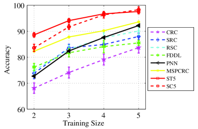
Figure 5: Aveage recognition accuracies (%) of 5 independent runs on AR dataset with number of training samples per class from 2 to 5. Standard deviations are shown with error bars. Results for PNN and MSPCRC are cited from [36] with the same setting, where the deviation results are not shown here due to their large values.

4.4 LFW-a

The original LFW database [12] contains images of 5,749 subjects in unconstrained environment. With the same settings as in [36], here we use LFW-a, an aligned version of LFW using commercial face alignment software [27]. A subset of LFW-a including 158 subjects with each subject more than 10 samples are used. The images are cropped to $121\times 121$ pixels. Following the settings in [36], 2 to 5 samples are randomly selected for training and another 2 samples for testing. All the images are finally resized to $32\times 32$.

Fig. 6 lists the average results of 5 independent runs. Similar results are obtained as in Fig. 5. Our methods perform considerably better than all other methods with even larger gaps on this challenging dataset. Same as on the AR dataset, soft threshold encoding achieves slightly better results than sparse coding here. On this dataset, residual based methods (even MSPCRC and PNN that use local patches) obtain poor results. With 5 training samples each class, our approach with soft threshold encoding outperforms the state-of-the-art method MSPCRC by around 29%.

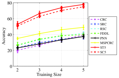
Figure 6: Average recognition accuracies (%) of 5 independent runs on the LFW-a dataset. Standard deviations are shown with error bars. Results for PNN and MSPCRC are cited from [3] with the same setting.

4.5 Feature combination

All the previous evaluations are based on raw intensity. To achieve better performance, multiple complementary features can be extracted for input of the feature learning pipeline. In this experiment, we take local binary patterns (LBP) for example to test the performance by feature fusion. We first represent each image as an LBP code image, and then apply the feature learning pipeline on images of raw pixels and LBP codes independently. The learned feature vectors through the two channels for each image are then concatenated into one large vector.

Table 9 shows the compared results between raw intensity and its fusion with LBP. Soft threshold is used for feature encoding. On both AR and LFW-a, the fused features obtain improved accuracies with all training sizes. For example with 2 training samples each class on LFW-a, the accuracy is averagely increased by 1.7% with the combined feature. It is an interesting research topic to explore how to improve the classification by combining more low-level image statistics. We leave this as a future research topic.

Training size	2	3	4	5
AR (Raw)	$88.6\pm 0.9$	$94.1\pm 0.8$	$96.7\pm 0.9$	$97.6\pm 0.9$
AR (Raw + LBP)	$89.2\pm 2.4$	$95.1\pm 1.1$	$97.9\pm 1.0$	$98.3\pm 0.6$
LFW-a (Raw)	$52.9\pm 3.5$	$66.5\pm 2.9$	$73.8\pm 1.8$	$77.9\pm 1.5$
LFW-a (Raw + LBP)	$54.6\pm 2.7$	$66.8\pm 1.9$	$74.6\pm 2.5$	$78.9\pm 1.8$

Table 9: Average results (%) of 5 runs on AR and LFW-a with fusion of learned features. The first column shows the training size per class. Soft threshold is used for encoding.

4.6 Modular methods vs. our pipeline

In this experiment, we want to compare our approach against the modular approach which is also based on local patches.

The modular approach has been widely used for robust face recognition. For example, the voting strategy is used to aggregate the intermediate results on local patches in [28, 34], which achieved much better results than the original methods on occlusion problems. For efficiency, here we take CRC [34] for example to compare the modular approach with our image classification model on the AR dataset. Local patches are densely extracted from the images of $32\times 32$ pixels with a stride of 1 pixel. The comparative results with different patch sizes are shown in Fig. 7. In addition to voting, we also conduct the modular approach by combining the residuals of all local patches for classification (‘Sum’ in the figure). The observations are:

1. Our generic image classification model achieves significantly better results than the modular approaches with all the setting of different patch sizes.

2. Our approach tends to achieve better results with smaller patches while the modular approaches favour mid-size patches. This is mainly due to the spatial pyramid pooling step in our pipeline. It remains unclear how to introduce spatial pooling into the residual based approaches such as SRC and CRC.

3. Also note that the simple sum operation consistently obtains higher accuracies than the majority voting method in the modular approaches.

This experiment shows that besides the advantage of local patches, other components in our pipeline such as feature encoding and spatial pooling must have contributed to the superior performance of the image classification pipeline for face recognition.

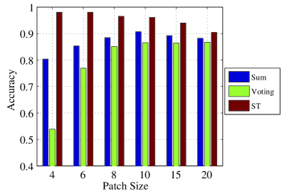
Figure 7: Comparison between modular methods (with ‘Votin’g and ‘Sum’ strategy) and our model (with soft threshold encoding) on the AR dataset. The patch size varies from $4\times 4$ to $20\times 20$ pixels.

5 Conclusion

Can face images be classified using the same strategy as in generic image classification? In this work, we have answered this question by applying the generic image classification pipeline to face recognition, which outperforms all the reported state-of-the-art face recognition methods by large margins on four standard benchmark datasets.

A large body of recent published face recognition methods, especially SRC-scheme based ones, have focused on designing complex dictionaries (e.g., using discriminant learning or K-SVD etc). By a thorough cross evaluation of the components in the image classification pipeline on face recognition problems, we show that the choice of dictionary learning algorithms is less critical than that of encoders. In particular, we show that randomly selected patches can work very well. Interestingly, we find that the dictionary is even not necessarily generated using patches extracted from face images. That is, a face image can be recognised using a representation generated from non-face image patches.

Another finding of this work is that the simple and efficient soft threshold algorithm surprisingly obtains on par results with the expensive $L_{1}$-constrained sparse coding. Note that, the best results on some datasets that we have tested are obtained by the components of a dictionary of randomly selected patches, soft threshold encoding, and pooling, followed by a simple linear classifier. In this entire procedure, the only component involving ‘learning’ is the simple linear classifier training.

In the future, we plan to explore the performance of multiple-layer hierarchical feature learning for face recognition. Our initial experiments on learning two-layer features using the approach of [15] and sparse filtering of [22] did not improve the performance over the single-layer features of this work on the AR and LFW-a datasets. However, more thorough experiments are needed before we can draw a conclusion. The facial image descriptor extracted with the pipeline presented here has potentials for other faces-related applications, such as face detection, retrieval, alignment, and tagging. Our preliminary experiments show very encouraging results on large-scale face image retrieval.

References

- [1] M. Aharon, M. Elad, and A. Bruckstein. K-SVD: an algorithm for designing overcomplete dictionaries for sparse representation. IEEE Trans. Signal Processing, 54(11):4311–4322, 2006.
- [2] T. Ahonen, A. Hadid, and M. Pietikainen. Face description with local binary patterns: application to face recognition. IEEE Trans. Pattern Anal. Mach. Intell., 28(12):2037–2041, 2006.
- [3] Y. Boureau, F. Bach, Y. LeCun, and J. Ponce. Learning mid-level features for recognition. In Proc. IEEE Conf. Comp. Vis. Patt. Recogn., pages 2559–2566, 2010.
- [4] C. Chen, C. Wei, and Y. Wang. Low-rank matrix recovery with structural incoherence for robust face recognition. In Proc. IEEE Conf. Comp. Vis. Patt. Recogn., pages 2618–2625, 2012.
- [5] A. Coates and A. Ng. The importance of encoding versus training with sparse coding and vector quantization. In Proc. Int. Conf. Mach. Learn., pages 921–928, 2011.
- [6] A. Coates, A. Ng, and H. Lee. An analysis of single-layer networks in unsupervised feature learning. In Proc. Int. Conf. Artif. Intell. Stat., pages 215–223, 2011.
- [7] W. Deng, J. Hu, and J. Guo. Extended SRC: undersampled face recognition via intra-class variant dictionary. IEEE Trans. Pattern Anal. Mach. Intell., page 1, 2012.
- [8] W. Deng, J. Hu, and J. Guo. In defense of sparsity based face recognition. In Proc. IEEE Conf. Comp. Vis. Patt. Recogn., 2013.
- [9] R. Fan, K. Chang, C. Hsieh, X. Wang, and C. Lin. Liblinear: a library for large linear classification. J. Mach. Learn. Res., pages 1871–1874, 2008.
- [10] A. Georghiades, P. Belhumeur, and D. Kriegman. From few to many: illumination cone models for face recognition under variable lighting and pose. IEEE Trans. Pattern Anal. Mach. Intell., 23(6):643–660, 2001.
- [11] Y. Gong and S. Lazebnik. Comparing data-dependent and data-independent embeddings for classification and ranking of internet images. In Proc. IEEE Conf. Comp. Vis. Patt. Recogn., pages 2633–2640, 2011.
- [12] G. Huang, M. Ramesh, T. Berg, and E. Learned-Miller. Labeled faces in the wild: a database for studying face recognition in unconstrained environments. In Faces in Real-Life Images Workshop in European Conference on Computer Vision, 2008.
- [13] A. Hyvarinen and E. Oja. Independent component analysis: algorithms and applications. Neural Netw., 13(4-5):411–430, 2000.
- [14] Z. Jiang, Z. Lin, and L. Davis. Learning a discriminative dictionary for sparse coding via label consistent K-SVD. In Proc. IEEE Conf. Comp. Vis. Patt. Recogn., pages 1697–1704, 2011.
- [15] R. Kiros and C. Szepesvári. Deep representations and codes for image auto-annotation. In Proc. Advances in Neural Information Process. Syst., pages 917–925, 2012.
- [16] R. Kumar, A. Banerjee, B. Vemuri, and H. Pfister. Maximizing all margins: pushing face recognition with kernel plurality. In Proc. IEEE Int. Conf. Comp. Vis., pages 2375–2382, 2011.
- [17] M. Lades, J. Vorbruggen, J. Buhmann, J. Lange, C. von der Malsburg, R. Wurtz, and W. Konen. Distortion invariant object recognition in the dynamic link architecture. IEEE Trans. Comput., 42(3):300 –311, 1993.
- [18] S. Lazebnik, C. Schmid, and J. Ponce. Beyond bags of features: spatial pyramid matching for recognizing natural scene categories. In Proc. IEEE Conf. Comp. Vis. Patt. Recogn., volume 2, pages 2169–2178, 2006.
- [19] L. Ma, C. Wang, B. Xiao, and W. Zhou. Sparse representation for face recognition based on discriminative low-rank dictionary learning. In Proc. IEEE Conf. Comp. Vis. Patt. Recogn., pages 2586–2593, 2012.
- [20] A. Martinez and R. Benavente. The AR Face Database. CVC, Tech. Rep., 1998.
- [21] I. Naseem, R. Togneri, and M. Bennamoun. Linear regression for face recognition. IEEE Trans. Pattern Anal. Mach. Intell., 32(11):2106–2112, 2010.
- [22] J. Ngiam, P. Koh, Z. Chen, S. Bhaskar, and A. Ng. Sparse filtering. In Proc. Advances in Neural Information Process. Syst., 2011.
- [23] P. Phillips, H. Wechsler, J. Huang, and P. Rauss. The feret database and evaluation procedure for face-recognition algorithms. Image and Vision Computing, 16(5):295–306, 1998.
- [24] Q. Shi, A. Eriksson, A. van den Hengel, and C. Shen. Is face recognition really a compressive sensing problem? In Proc. IEEE Conf. Comp. Vis. Patt. Recogn., pages 553–560, 2011.
- [25] I. Theodorakopoulos, I. Rigas, G. Economou, and S. Fotopoulos. Face recognition via local sparse coding. In Proc. IEEE Int. Conf. Comp. Vis., pages 1647–1652, 2011.
- [26] J. Wang, J. Yang, K. Yu, F. Lv, T. Huang, and Y. Gong. Locality-constrained linear coding for image classification. In Proc. IEEE Conf. Comp. Vis. Patt. Recogn., pages 3360 –3367, 2010.
- [27] L. Wolf, T. Hassner, and Y. Taigman. Similarity scores based on background samples. In Proc. Asian conf. Computer Vision, pages 88–97. 2010.
- [28] J. Wright, A. Yang, A. Ganesh, S. Sastry, and Y. Ma. Robust face recognition via sparse representation. IEEE Trans. Pattern Anal. Mach. Intell., 31:210–227, 2009.
- [29] J. Yang, J. Yang, and A. Frangi. Combined fisherfaces framework. Image and Vision Computing, 21(12):1037–1044, 2003.
- [30] J. Yang, K. Yu, Y. Gong, and T. Huang. Linear spatial pyramid matching using sparse coding for image classification. In Proc. IEEE Conf. Comp. Vis. Patt. Recogn., pages 1794–1801, 2009.
- [31] M. Yang and L. Zhang. Gabor feature based sparse representation for face recognition with gabor occlusion dictionary. In Proc. Eur. Conf. Comp. Vis., pages 448–461, 2010.
- [32] M. Yang, L. Zhang, X. Feng, and D. Zhang. Fisher discrimination dictionary learning for sparse representation. In Proc. IEEE Int. Conf. Comp. Vis., pages 543–550, 2011.
- [33] M. Yang, L. Zhang, J. Yang, and D. Zhang. Robust sparse coding for face recognition. In Proc. IEEE Conf. Comp. Vis. Patt. Recogn., pages 625–632, 2011.
- [34] L. Zhang, M. Yang, and X. Feng. Sparse representation or collaborative representation: Which helps face recognition? In Proc. IEEE Int. Conf. Comp. Vis., pages 471–478, 2011.
- [35] Q. Zhang and B. Li. Discriminative K-SVD for dictionary learning in face recognition. In Proc. IEEE Conf. Comp. Vis. Patt. Recogn., pages 2691–2698, 2010.
- [36] P. Zhu, L. Zhang, Q. Hu, and S. Shiu. Multi-scale patch based collaborative representation for face recognition with margin distribution optimization. In Proc. Eur. Conf. Comp. Vis., pages 822–835, 2012.