draft=false, abstract=true, numbers=enddot section subsection

A nice limaçon-like spiral

Abstract

A limaçon-like curve, allowing $2\pi$-transition with monotone curvature between concentric curvature elements, is presented. The curve is 4th degree algebraic, 4th degree rational, and shares other common features with Pascal’s limaçon.

We present a family of curves, traced in polar coordinates $(r,\xi)$ as

$$r(\xi)=f\left(\mu\cos\xi+\sqrt{2-\cos^{2}\xi}\right),\qquad\mu\lesseqgtr 0.$$

Dimensionless parameter $\mu$ controls the shape of the curve. Implicit equation looks like

$$\left(x^{2}+y^{2}-\mu fx\right)^{2}=f^{2}(x^{2}+{\color[rgb]{1,0,0}\underline{{\color[rgb]{0,0,0}2}}}y^{2}),$$ (1)

and rational parametrization is

$$x(t)=f\dfrac{\left(t^{2}-1\right)\,\left[(\mu-1)t^{2}-(\mu+1)\right]}{t^{4}+1},\quad y(t)=f\sqrt{2}\,\dfrac{t\left[(\mu-1)t^{2}-(\mu+1)\right]}{t^{4}+1}.$$

Underlined factor $2$ in Eq. (1) distinguishes this curve from Pascal’s limaçon [1], and provides a nice property: extremal circles of curvature are concentric, and the curve performs $G^{3}$-continuous transition between them. If they are equally directed $(\left\lvert\mu\right\rvert>1)$, the transition is spiral, i. e. curvature varies monotonically. Total turning angle is in this case $2\pi$.

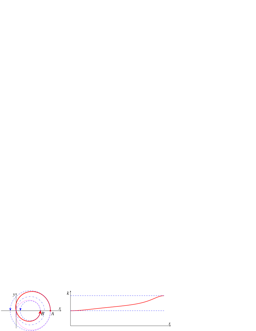
Fig. 1: Spiral transition (heavy curve), its circles of curvature (dashed), their midcircle (dotted-dashed). Plot of curvature $k$ vs arc length $s$.

The transition is shown as curve $\displaystyle{\buildrel\,\,\frown\over{AB}}$ in Fig. 1. The whole limaçon includes the second arc, symmetric about the $x$-axis. Curvature elements at the endpoints $A$ and $B$ are written below as $\left\{x,y,\tau,k\right\}$, where $\tau$ defines the unit tangent $(\cos\tau,\sin\tau)^{T}$, and $k$ is curvature. Common center of two circles is denoted as $x_{c}$:

$$\begin{array}[]{lllll}\xi=0:&\left\{\vphantom{\dfrac{\pi}{2}}f(\mu+1),\right.&0,&\dfrac{\pi}{2}\mathop{\rm sgn}\nolimits[f(\mu+1)],&\dfrac{2\mu}{\left\lvert f\right\rvert\,\left\lvert\mu+1\right\rvert(\mu+1)}\left.\vphantom{\dfrac{\pi}{2}}\right\};\\[4.30554pt] \xi=\pi:&\left\{\vphantom{\dfrac{\pi}{2}}f(\mu-1),\right.&0,&\dfrac{\pi}{2}\mathop{\rm sgn}\nolimits[f(\mu-1)],&\dfrac{2\mu}{\left\lvert f\right\rvert\,\left\lvert\mu-1\right\rvert(\mu-1)}\left.\vphantom{\dfrac{\pi}{2}}\right\};\end{array}\qquad x_{c}=f\frac{\mu^{2}-1}{2\mu}.$$

Any ratio of curvatures of concentric circles (except $\pm 1$) can be reached with proper $\mu$:

$$\frac{k(\pi)}{k(0)}=\pm\kappa^{2}{:}\quad\pm\kappa^{2}=\frac{\mu+1}{\mu-1}\cdot\left\lvert\frac{\mu+1}{\mu-1}\right\rvert\quad\Longrightarrow\quad\mu=\frac{\left\lvert\kappa\right\rvert\pm 1}{\left\lvert\kappa\right\rvert\mp 1}$$

(the limit case $f\to 0$, $\mu\to\infty$, $\mu f=2R=\operatorname{const}$, yields the ratio $+1$, and limaçon (1) degenerates into duplicated circle $(x^{2}+y^{2}-2Rx)^{2}=0$).

The limaçon is the inverse, with respect to the circle $x^{2}+y^{2}=f^{2}$, of conic (2), which has excentricity $e$, focal parameter $p$, and the focii at the points $(x_{f},0)$:

$$2y^{2}+(1-\mu^{2})x^{2}+2\mu fx-f^{2}=0,\qquad e=\sqrt{\frac{\mu^{2}+1}{2}},\quad p=\frac{1}{2}f,\quad x_{f}=\frac{f}{2(\mu\pm e)}.$$ (2)

The former vertical axis of symmetry of the conic was equally a trivial midcircle of two extremal circles of curvature. After inversion it appears in Fig. 1 as the midcircle of two extremal (concentric) circles of curvature, and as the circle of symmetry of the whole limaçon.

Note that Pascal’s limaçon was obtained by inversion of conic with the center of inversion in the focus. In (2) the focus is on the $x$-axis at some distance $x_{f}\neq 0$ from the center of inversion.

The polar equation $\rho(\theta)$ of the limaçon with the pole in the common center $x_{c}$ is given by

$$4\mu^{2}\rho^{2}(\theta)-4\mu f\left(\cos\theta+\mu\sqrt{\mu^{2}+\sin^{2}\theta}\right)\rho(\theta)+(\mu^{2}-1)^{2}f^{2}=0.$$

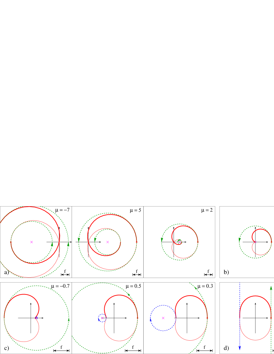
Fig. 2: Concentric limaçons, produced by inversion of: a) hyperbola; b) parabola; c,d) ellipse.

Fig. 2 shows the variety of shapes of the limaçon.

• Curves with $\left\lvert\mu\right\rvert>1$ inherit two vertices from the original hyperbola, as well as spirality of the transition between them. Point $(0,0)$ is self-intersection.

• In the parabolic case $\left\lvert\mu\right\rvert=1$ the inner concentric circle degenerates into a cusp at the point $(0,0)$. Two halves of the limaçon remain spirals, as two halves of the parabola were.

• When $\left\lvert\mu\right\rvert<1$, the concentric circles of curvature have opposite orientations. Such boundary conditions contradict to spirality. To enable connection, conic (2) turns into ellipse, and each branch of the limaçon makes use of additional vertex. Point $(0,0)$ is isolated singularity. The special case $\mu=0$ is a particluar case of elliptic lemniscate [1].

The curve was initially obtained from a close look at the critical solution of the method [2], described there as $\sigma=\pi$. Together with concentric given data, the solution promised to be simple and interesting. For normalized (in terms of [2]) boundary conditions

$$\left\{-1,\>0,\>{-\dfrac{\pi}{2}},\>\dfrac{\kappa^{2}-1}{2\kappa^{2}}\right\}\quad\text{and}\quad\left\{1,\>0,\>{-\dfrac{\pi}{2}},\>\dfrac{\kappa^{2}-1}{2}\right\},\quad\text{with common center}\;\left(\frac{\kappa^{2}+1}{\kappa^{2}-1},\,0\right),$$

the method returns parametrization

$$x(u)=\frac{\kappa+1}{\kappa-1}+\frac{2\kappa}{\kappa-1}\cdot\frac{(1-2u)\left[u^{2}\kappa-(1-u)^{2}\right]}{\kappa^{2}u^{4}+(1-u)^{4}},\quad y(u)=\frac{-2\sqrt{2\kappa^{3}}}{\kappa-1}\cdot\frac{u(1-u)(1-2u)}{\kappa^{2}u^{4}+(1-u)^{4}}.$$

The sought for spiral connection corresponds to $0\leqslant u\leqslant 1$.

In common geometric terms, the curve could be constructed as follows. Consider canonical hyperbola $\frac{x^{2}}{a^{2}}-\frac{y^{2}}{b^{2}}=1$. Let $p$, $e$, and $z(t)=x(t)+iy(t)$ be its focal parameter, excentricity, and parametrization. Choose the circle of inversion, centered on the $x$-axis at the point $(x_{0},0)=(\mu p,0)$. The inverse curve $\widetilde{z}(t)$ can be obtained, e. g., as $\frac{p^{2}}{z(t)-x_{0}}$, which also includes reflection about the $x$-axis, and translation, such that the image of the former infinite point is shifted from $(x_{0},0)$ to the coordinate origin. The parameter values $t_{1,2}$, corresponding to vertices of the hyperbola, remain such for the curve-image. Calculating curvature elements at $\widetilde{z}(t_{1})$ and $\widetilde{z}(t_{2})$, and equating the centers of curvature, results in condition

$$2e^{2}=\mu^{2}+1.$$

So, special choice of excentricity solves the problem of concentricity.