Abstract: In order to bring contraction analysis into the very fruitful and topical fields of stochastic and Bayesian systems, we extend here the theory describes in [Lohmiller and Slotine, 1998] to random differential equations. We propose new definitions of contraction (almost sure contraction and contraction in mean square) which allow to master the evolution of a stochastic system in two manners. The first one guarantees eventual exponential convergence of the system for almost all draws, whereas the other guarantees the exponential convergence in $L_{2}$ of the system to a unique trajectory. We then illustrate the relative simplicity of this extension by analyzing usual deterministic properties in the presence of noise. Specifically, we analyze stochastic gradient descent, impact of noise on oscillators synchronization and extensions of combination properties of contracting systems to the stochastic case. This is a first step towards combining the interesting and simplifying properties of contracting systems with the probabilistic approach.

Key-words: random differential equations, contraction theory

Analyse de la contraction pour les systèmes dynamique alétoires non-linéaires

Résumé : La théorie de la contraction ([Lohmiller and Slotine, 1998] ) sert à l’étude de la stabilité des systèmes dynamiques non-linéaires. Dans ce rapport, nous étendons la théorie de la contraction aux cas des équations différentielles aléatoires. Nous proposons deux nouvelles définitions de la contraction dans un cadre aléatoire (contraction presque sûre, et contraction aux moindres carrés) qui permettent de controler l’évolution d’un système stochastique de deux manières. La première garantie la convergence exponentielle pour presque toutes les réalisations du sysème, tandis que la deuxième garantie la convergence dans $L_{2}$ à une trajectoire unique. Nous illustrons enfin la relative simplicité de cette extension en analysant des propriétés déterministes bien connu dans un cadre bruité. Plus spécifiquement, nous alnalysong la descente de gradient stochastique, l’impact du bruit sur la synchronisation d’oscillateurs et l’extension des propriétés de combinaison de systèmes contractant aux cas stochastique.

Mots-clés : équations différentielles aléatoires, théorie de la contraction

1 Introduction

The concept of random dynamical systems appeared to be a useful tool for modelers of many different fields, especially in computational neuroscience. Indeed, introducing noise in a system can be either a way to describe reality more sharply or to generate new behaviors absent from the deterministic world. Naively, the definition of such systems generalized the usual deterministic one as follows,

$${\bf x}_{i+1}={\bf f}_{i}({\bf x}_{i},i,\mbox{\boldmath$\xi$}_{i}(\omega))\qquad\mbox{or}\qquad\dot{\bf x}_{t}={\bf f}({\bf x}_{t},\mbox{\boldmath$\xi$}_{t}(\omega),t)$$ (1)

where $\mbox{\boldmath$\xi$}_{i}$ (resp. $\mbox{\boldmath$\xi$}_{t}$) defines a discrete (resp. continuous) stochastic process.

Unfortunately, it comes out that whereas the extension of the definition in the discrete time case is rather straightforward, things get much harder for continuous time. Indeed, equation 1 does not make sense for every continuous stochastic process. There are basically to different ways of fixing this problem :

1. One can restrict the definition to sufficiently smooth stochastic processes, namely those whose trajectories are cadlag (see subsection 2.3). This gives rise to random differential equations.

2. Or, as important stochastic processes like White noise do not satisfy this property, one can switch to stochastic differential equations and Itô calculus.

When first looking at it, Itô calculus seems more accurate as it just generalized the usual differential calculus. But the problem of this formalism lies in the absence of “realisability” of such defined systems. By realisability, we mean the ability to simulate the behavior of a system by mean of a computer. Hence, all result we can obtain are purely theoretic, and it is hard to make up an intuition on how such a system evolves. From a modeling point of view, this lake of manageability make this formalism unusable in most fields as we are hardly able to find explicit solution of a huge dynamical system as encountered in biology, and thus even in the deterministic case. It follows that we need our system to be realizable, and so we must restrict our attention to random differential equations.

Once this restriction performed, we can really solve our system with the traditional tools of differential analysis. Indeed, it now makes sense to fix a draw in the probability space and solve the equation as the noise being an external input. We can thus describes the trajectory of the system given a sample path of the stochastic process. It results that we are also able to use deterministic contraction theory to study stability when the noise never put the system out of contraction bounds. But this implies that every trajectory is contracting, and so noise does not really matter.

In this paper, we will investigate new definitions of stochastic stability together with sufficient condition to guarantee that a random differential system as a nice behavior even if the noise can induce partial divergence in the trajectories.

The notations of this paper follow those of the keystone [Arnold, 1998].

2 Part 1 : State’s dependency

2.1 Nonlinear random system : the discrete time case

2.1.1 Almost sure contraction : asymptotic exponential convergence a.s.

As a first step, we define the stochastic contraction in the field of discrete system. In that case, there is no problem regarding the equation generating the dynamic system as it is just the iterated application of possibly different functions. We are dealing with stochastic processes of the form :

$$\mbox{\boldmath$\xi$}:\Omega\times\mathbb{N}\rightarrow\mathbb{R}^{n}$$

ie. we assume $\xi$ to be equivalent to a sequence of random variable $\mbox{\boldmath$\xi$}_{i}:\Omega\rightarrow\mathbb{R}^{n}$.

The definition of contraction in discrete-time case is a direct extension of the deterministic case and makes use of the notion of discrete stochastic differential systems ([Jaswinski, 1970]) of the form

$${\bf x}_{i+1}={\bf f}_{i}({\bf x}_{i},i,\mbox{\boldmath$\xi$}_{i}(\omega))$$

where the ${\bf f}_{i}$ are continuously differentiable (a condition that will be assumed in the rest of this paper).

This definition is the natural extension of the definition of [Lohmiller and Slotine, 1998], which assessed that the the difference between two trajectories tends to zero exponentially fast. In the stochastic case, we look for similar conditions satisfy almost surely.

First, we have to reformulate the traditional property satisfied by the metric allowing a space deformation. In the deterministic case, the metric $M_{i}({\bf x}_{i},i)$ has to be uniformly positive definite with respect to ${\bf x}_{i}$ and $i$. This property of uniformity for a metric $M_{i}({\bf x},i,\mbox{\boldmath$\xi$}_{i})$ depending also on noise can be written

$$\exists\lambda\quad\forall{\bf x},i\quad M({\bf x},i,{\bf\mbox{\boldmath$\xi$}}_{i})\geq\lambda{\bf I}\quad\mbox{a.s.}$$

But as we want the noise to introduce local bad behaviors, we need to relax the property in a sense that contraction can only been guaranteed asymptotically. This introduces a slightly difficulty as the naive formulation

$$\exists 0\leq\alpha<1\qquad\lim_{n\rightarrow\infty}(\|\delta{\bf z}\|-\|\delta{\bf z}_{o}\|\alpha^{n})=0$$

just says that $\|\delta{\bf z}\|$ tends to zero, which is not what we want. We thus have to switch to the following refined formulation.

Definition 1

The random system ${\bf x}_{i+1}={\bf f}_{i}({\bf x}_{i},i,\mbox{\boldmath$\xi$}_{i}(\omega))$, is said to be almost surely contracting if there exists a uniformly positive definite metric $M_{i}({\bf x},i,\mbox{\boldmath$\xi$}_{i})$ and $\eta<0$ such that:

$$\mathbb{P}\{\omega\in\Omega,\ \limsup_{n\rightarrow\infty}\frac{1}{n}\log(\|\delta{\bf z}\|)\leq\eta\}=1$$

ie. the difference between two trajectories tends almost surely to zero exponentially.

Remark 1

1. The notion of contracting region cannot be extended to stochastic case as it is hardly possible to guarantee that a stochastic trajectory stay in a bowl without requiring strong bound on the noise. And in that case, the noise can be treated as a bounded perturbation by analyzing the worst case.

2. The definition makes use of logarithm whereas $\|\delta{\bf z}\|$ can be equal to $0$. Nevertheless, the reader should not be deterred and each time such a case appears, the equation is also satisfy if we allow infinite value and basic analytic extension (for example, $\mathbb{E}(\log\alpha)=-\infty$ as soon as $\alpha(\omega)=0$ for some $\omega$).

We can now state the first theorem of this paper. Remark that in the definition of the system below, the dependence on the stochastic perturbation is almost linear, as we can not master a malicious non-linear system which strongly use the “bad draw” of the stochastic process to diverge. In a sense, the system must satisfy a notion of uniformity with respect to the stochastic process.

Theorem 1

Given the random system ${\bf x}_{i+1}={\bf f}_{i}({\bf x}_{i},i,\mbox{\boldmath$\xi$}_{i}(\omega))$, note $\sigma_{f}({\bf x}_{i},i,\mbox{\boldmath$\xi$}_{i})$ the largest singular value of the generalized Jacobian of ${\bf f}_{i}$ at time i according to some metric $M_{i}({\bf x},i,\mbox{\boldmath$\xi$}_{i})$.

A sufficient condition for the system to be almost surely contracting is that

• the random process $\sigma_{f_{i}}({\bf x},i,\mbox{\boldmath$\xi$}_{i})$ can be bounded independently from ${\bf x}$, ie there exists a stochastic process $\eta_{i}$ such that

  $$\forall{\bf x}\quad\sigma_{f_{i}}({\bf x},i,\mbox{\boldmath$\xi$}_{i})\leq\eta_{i}\qquad\mbox{a.s.}$$

• the stochastic process $\log(\eta_{i})$ follows the strong law of large number (eg. i.i.d.)

  $$\frac{1}{n}\sum_{i=1}^{n}\log(\eta_{i})\rightarrow\frac{1}{n}\sum_{i=1}^{n}\mathbb{E}(\log(\eta_{i}))\qquad\mbox{a.s.}$$

• the expectation of the random variables $\log(\eta_{i})$ can be uniformly bounded by some $\eta<0$

  $$\forall i\quad\mathbb{E}(\log(\eta_{i}))\leq\eta$$

Proof 1

Proof.

We make a strong use of the basic idea of the original proof.

Note $F_{i}$ the discrete generalized Jacobian of $f_{i}$ : $F_{i}({\bf x},i,\mbox{\boldmath$\xi$}_{i})\ =\ \Theta_{i+1}\frac{\partial}{\partial{\bf x}}{\bf f}_{i}({\bf x},i,{\bf\mbox{\boldmath$\xi$}}_{i})\Theta^{-1}_{i}$ we have:

$$\begin{array}[]{lrcl}&{\bf\delta{\bf z}}_{i+1}^{T}{\bf\delta{\bf z}}_{i+1}&=&{\bf\delta{\bf z}}_{i}^{T}(F_{i}^{T}F_{i})\ {\bf\delta{\bf z}}_{i}\\ \\ \Rightarrow&{\bf\delta{\bf z}}_{i+1}^{T}{\bf\delta{\bf z}}_{i+1}&\leq&\sigma^{2}_{f_{i}}({\bf x}_{i},i,\mbox{\boldmath$\xi$}_{i})\ {\bf\delta{\bf z}}_{i}^{T}{\bf\delta{\bf z}}_{i}\qquad\mbox{a.s.}\end{array}$$

and hence,

$$\|\delta{\bf z}_{n}\|^{2}\leq\|\delta{\bf z}_{o}\|^{2}\prod_{i=0}^{n}\sigma^{2}_{f_{i}}({\bf x}_{i},i,\mbox{\boldmath$\xi$}_{i})\qquad\mbox{a.s.}$$

So by monotony of logarithm and the two required properties, we can deduce that for almost every $\omega$

$$\begin{array}[]{rcl}\limsup_{n\rightarrow\infty}\frac{1}{n}\log(\|\delta{\bf z}_{n}\|)&\leq&\limsup_{n\rightarrow\infty}\frac{1}{n}\log(\prod_{i=0}^{n}\sigma_{f_{i}}({\bf x}_{i},i,{\bf\mbox{\boldmath$\xi$}}_{i}))\\ &\leq&\limsup_{n\rightarrow\infty}\frac{1}{n}\sum_{i=0}^{n}\log(\eta_{i})\\ &=&\limsup_{n\rightarrow\infty}\frac{1}{n}\sum_{i=0}^{n}\mathbb{E}(\log(\eta_{i}))\\ &\leq&\eta\\ \end{array}$$

That is

$$\mathbb{P}\{\omega\in\Omega,\ \limsup_{n\rightarrow\infty}\frac{1}{n}\log(\|\delta{\bf z}\|)\leq\eta\}=1$$

$\square$

2.1.2 Contraction in mean square: asymptotic exponential convergence in mean square

We have seen in the subsection above sufficient conditions to guarantee almost sure asymptotic exponential convergence. But we could also be interested in looking for conditions to guarantee exponential convergence in mean square. That’s what we are trying to capture with the notion of contraction in mean square.

Definition 2

The random system ${\bf x}_{i+1}={\bf f}_{i}({\bf x}_{i},i,\mbox{\boldmath$\xi$}_{i}(\omega))$, is said to be contracting in mean square if there exists an uniformly positive definite metric $M_{i}({\bf x},i,\mbox{\boldmath$\xi$}_{i})$ such that:

$$\exists 0\leq\eta<1\quad\mathbb{E}(\|\delta{\bf z}(i,\mbox{\boldmath$\xi$}_{i})\|^{2})\leq\|\delta{\bf z}_{o}\|^{2}\eta^{i}$$

Theorem 2

Given the random system , ${\bf x}_{i+1}={\bf f}_{i}({\bf x}_{i},i,\mbox{\boldmath$\xi$}_{i}(\omega))$ note $\sigma_{f_{i}}({\bf x},i,\mbox{\boldmath$\xi$}_{i})$ the largest singular value of the generalized Jacobian of ${\bf f}_{i}$ at time i according to some metric $M$.

A sufficient condition for the system to be contracting in mean square is that

• the random process $\sigma_{f_{i}}({\bf x},i,\mbox{\boldmath$\xi$}_{i})$ can be bounded independently from ${\bf x}$, ie there exists a stochastic process $\eta_{i}$ such that

  $$\forall{\bf x}\quad\sigma_{f_{i}}({\bf x},i,\mbox{\boldmath$\xi$}_{i})\leq\eta_{i}\qquad\mbox{a.s.}$$

• the stochastic process $\eta_{i}$ is constituted of independent random variables

• the expectation of the random variables $\eta_{i}^{2}$ can be uniformly bounded by some $0\leq\eta<1$

  $$\forall i\quad\mathbb{E}(\eta_{i}^{2})\leq\eta$$

Proof 2

Proof. Note $F_{i}$ the discrete generalized Jacobian of $f_{i}$, we have again

$${\bf\delta{\bf z}}_{i+1}^{T}{\bf\delta{\bf z}}_{i+1}\leq\sigma^{2}_{f_{i}}({\bf x}_{i},i,\mbox{\boldmath$\xi$}_{i})\ {\bf\delta{\bf z}}_{i}^{T}{\bf\delta{\bf z}}_{i}\leq\eta_{i}^{2}\ {\bf\delta{\bf z}}_{i}^{T}{\bf\delta{\bf z}}_{i}\qquad\mbox{a.s.}$$

Introducing the expectation value of $\|\delta{\bf z}\|^{2}$, we use that independence between $X$ and $Y$ is defined as the uncorrelation of $f(X)$ and $g(Y)$ for all mesurable functions $f$ anf $g$.

$$\mathbb{E}(\|{\bf\delta{\bf z}}_{i+1}\|^{2})\ \leq\ \mathbb{E}(\eta_{i}^{2}\|{\bf\delta{\bf z}}_{i}\|^{2})=\mathbb{E}(\eta_{i}^{2})\mathbb{E}(\|{\bf\delta{\bf z}}_{i}\|^{2})$$

and hence

$$\mathbb{E}(\|\delta{\bf z}_{i}\|^{2})\leq\|\delta{\bf z}_{o}\|^{2}\eta^{i}$$

$\square$

2.2 Stochastic gradient

Let us have a look to a stochastic way of minimizing a function, highly used in computational neuroscience community, called stochastic gradient.

The idea is to use the traditional minimization by gradient descent but we want to avoid explicit computation of the gradient as it is generally of high cost or even infeasible. For that, we introduced a stochastic perturbation which has the role of a “random differentiation”.

Let $\hat{P}=P+\Pi$ be the perturbation of the state $P$ with respect the vector $\Pi$ of stochastic processes $\Pi_{i}$ . Define the discrete system

$$P_{n+1}=P_{n}-\mu.(\mathcal{E}(\hat{P_{n}})-\mathcal{E}(P_{n}))\Pi$$

with $\mu>0$.

Providing that the $\Pi_{i}$’s are mutually uncorrelated and of auto-correlation $\sigma^{2}$ (ie. $\mathbb{E}(\Pi_{i}.\Pi_{j})=\sigma^{2}.\delta_{i,j}$), the system satisfies:

$$\delta P_{n+1}=\delta P_{n}-\mu.(\sum_{k}\frac{\partial^{2}\mathcal{E}}{\partial p_{k}\partial p_{i}}(P^{*})\Pi_{k}.\Pi_{j})_{i,j}.\delta P_{n}$$

where $P^{*}$ is given by the finite difference theorem. So, by taking the expectation:

$$\mathbb{E}(\delta P_{n+1})=(I-\mu.\sigma^{2}.\frac{\partial^{2}\mathcal{E}}{\partial P_{n}^{2}}).\mathbb{E}(\delta P_{n})$$

So the system is contracting in mean square if

• $\frac{\partial^{2}\mathcal{E}}{\partial P_{n}^{2}}>0$ that is $\mathcal{E}$ is strictly convex.

• $\mu.\sigma^{2}\frac{\partial^{2}\mathcal{E}}{\partial P_{n}^{2}}<I$ (that is $\mu.\sigma^{2}$ sufficiently small)

2.3 Nonlinear random system : the continuous time case

We have seen in subsection 2.1 that the notion of contraction for discrete-time varying systems harmonizes well with stochastic calculus. Unfortunately the story is less straightforward in the continuous time case. Nevertheless, as outlined in introduction, for some practical reasons, we can restrict our intention to the case of random differential systems as define in [Arnold, 1998]. Let us briefly summarize the technical background.

We want to define the stochastic extension of deterministic differential systems as fellows.

$$\dot{\bf x}_{t}={\bf f}({\bf x}_{t},t,\mbox{\boldmath$\xi$}_{t}(\omega))$$ (2)

where $\mbox{\boldmath$\xi$}_{t}$ is a continuous stochastic process and ${\bf f}$ is a sufficiently smooth function, namely continuously differentiable with respect to ${\bf x}_{t}$ (the condition on ${\bf f}$ can be reduced to a lipschitz condition, but as we need differentiability in the rest of this paper, we prefer to assume it right now).

But this formulation does not make sense for every kind of continuous processes. Typically, when dealing with White noise process, the right-hand part of equation 2 does not present finite variation. In order to overcome this difficulty, we will assume that $\mbox{\boldmath$\xi$}_{t}$ is a “nice” stationary stochastic process whose trajectories are cadlag (for the french “continue à droite et avec des limites à gauche”), ie. are right continuous with left-hand limits.

Arnold proved in [Arnold, 1998] that under some assumption on ${\bf f}$, equation 2 admits a unique solution which is a global flow, whereas in general it is just a local flow.

Theorem 3 ([Arnold, 1998])

Suppose that $\xi$ is cadlag and ${\bf f}\in\mathcal{C}^{1}$. Then, equation 2 admit a unique maximal solution which is a local random dynamical system continuously differentiable. If furthermore ${\bf f}$ satisfies

$$\|{\bf f}(\mbox{\boldmath$\xi$},{\bf x})\|\leq\alpha(\mbox{\boldmath$\xi$})\|{\bf x}\|+\beta(\mbox{\boldmath$\xi$})$$

where $t\rightarrow\alpha(\mbox{\boldmath$\xi$}_{t}(\omega))$ and $t\rightarrow\beta(\mbox{\boldmath$\xi$}_{t}(\omega))$ are locally integrable, then the solution is a global RDS.

Thus, we cannot assume that random differential system defines a unique continuous trajectory for every $\omega$. This problem is also known in the deterministic case where Vidyasagar has shown the prevalence of differential equations despite our knowledge of only very restrictive characterization. Indeed, the set of equations admitting a unique solution is non-meager, whereas the set of equations we are able to exhibit is meager. That is, “practically all” equations admit a unique solution whereas we can characterize “practically none” of them ! So we will assume in the rest of this paper that the solution of the differential equation exists and is a unique continuously differentiable RDS.

All those restriction are rather technical and we refer the interesting reader to [Arnold, 1998] for further explanations. We can yet give two slogans reformulating intuitions coming from those restrictions :

The perturbation is memoryless

The noise appearing in the right-hand side of equation 2 is memoryless in the sense that only the value of the perturbation at time $t$ enters into the generator ${\bf f}$.

The perturbation do have small variations

The cadlag condition is a nice way to avoid problems generated by dramatically varying processes like White noise process while allowing interesting discontinuous processes such as jump Markov processes.

From now on, when we will talk about random differential system, we assume that the solution of equation 2 exists and is a unique continuously differentiable RDS. We also suppose that all the processes we are dealing with are stationary and have cadlag trajectories.

2.3.1 Almost sure contraction

We can now define the notion of almost sure contraction for the continuous-time case.

Definition 3

A random differential system $\dot{\bf x}_{t}={\bf f}({\bf x}_{t},t,{\bf\mbox{\boldmath$\xi$}}_{t}(\omega))$ is said to be almost surely contracting if there exists an uniformly positive definite metric $M({\bf x},t,\mbox{\boldmath$\xi$}_{t})$ and $\eta<0$ such that:

$$\mathbb{P}\{\omega\in\Omega,\ \limsup_{t\rightarrow\infty}\frac{1}{t}\log(\|\delta{\bf z}\|)\leq\eta\}=1$$

ie. the difference between two trajectories tends almost surely to zero exponentially.

We now state conditions for a system to be almost surely contracting. The traditional contraction analysis requires that the largest eigenvalue of the general Jacobian is uniformly bounded by a negative constant. The stochastic version of it mainly requires that the largest eigenvalue which define a process, is bounded by a process which follows the law of large number and of expectation uniformly negative.

Theorem 4

Given the system equations , $\dot{\bf x}_{t}={\bf f}({\bf x}_{t},t,{\bf\mbox{\boldmath$\xi$}}_{t}(\omega))$ note $\lambda_{f}({\bf x},t,\mbox{\boldmath$\xi$}_{t})$ the largest eigenvalue of the generalized Jacobian of ${\bf f}$ at time t according to some metric $M$.

A sufficient condition for the system to be almost surely contracting is that

• the random process $\lambda_{f}({\bf x},t,\mbox{\boldmath$\xi$}_{t})$ can be bounded independently from ${\bf x}$, ie there exists a stochastic process $\eta_{t}$ such that

  $$\forall{\bf x}\quad\lambda_{f}({\bf x},t,\mbox{\boldmath$\xi$}_{t})\leq\eta_{t}\qquad\mbox{a.s.}$$

• the stochastic process $\eta_{t}$ follows the strong law of large number

  $$\frac{1}{t}\int_{0}^{t}\eta_{t}\rightarrow\frac{1}{t}\int_{0}^{t}\mathbb{E}(\eta_{t})\qquad\mbox{a.s.}$$

• We can uniformly bound the expectation of the $\eta_{t}$ with some $\eta<0$

  $$\forall t\quad\mathbb{E}(\eta_{t})\leq\eta$$

Proof 3

Proof. We make a strong use of the basic idea of the original proof.

$$\frac{1}{2}\ \frac{d}{dt}({\bf\delta{\bf z}}^{T}{\bf\delta{\bf z}})\leq\lambda_{f}({\bf x}_{t},t,\mbox{\boldmath$\xi$}_{t})\ {\bf\delta{\bf z}}^{T}{\bf\delta{\bf z}}\qquad\mbox{a.s.}$$

and hence

$$\|\delta{\bf z}\|\leq\|\delta{\bf z}_{o}\|\ e^{\ \int\limits_{o}^{t}\eta_{t}dt}\qquad\mbox{a.s.}$$

Since $\eta_{t}$ verifies the law of large numbers, we have almost surely

$$\begin{array}[]{rcl}\limsup\frac{1}{t}\log\|\delta{\bf z}\|&\leq&\limsup\frac{1}{t}\int\limits_{o}^{t}\eta_{t}\ dt\\ &=&\limsup\frac{1}{t}\int\limits_{o}^{t}\mathbb{E}(\eta_{t})dt\\ &\leq&\eta\end{array}$$

$\square$

Remark 2

It is reassuring that if we take a continuous random system satisfying conditions above, then the “discrete envelop” defined by $X_{n+1}=\exp[\int_{P_{n}}\lambda_{f}({\bf x}_{t},t,\mbox{\boldmath$\xi$}_{t})]X_{n}$ is a discrete almost surely contracting system.

2.3.2 Contraction in mean square

As it is the case in discrete-time case, we would like to find sufficient that guarantee the contraction in mean square of our system

$$\mathbb{E}(\|\delta{\bf z}(t,{\mbox{\boldmath$\xi$}_{t}})\|^{2})\leq\|\delta{\bf z}_{o}\|^{2}e^{\eta t}$$ (3)

Unfortunately, we have seen that this property required discrete independent stochastic processes, whose continuous counterpart are processes like the White noise process. As we have refused to deal with that kind of processes, we need to find a stronger condition that yet ensure a similar constraint on the average trajectory.

That’s why we are moving to coarse-grained version of equation 3, namely where the property is guaranteed only for a discrete sample of the average trajectory. This property will be assessed when dealing with stochastic process which are coarse-grain independent, as define below.

Definition 4

A random differential system $\dot{\bf x}_{t}={\bf f}({\bf x}_{t},t,\mbox{\boldmath$\xi$}_{t}(\omega))$ is coarse-grain contracting if there exists a metric $M({\bf x},t,\mbox{\boldmath$\xi$}_{t})$ and a partition $t_{1}<t_{2}<\ldots$ such that:

$$\exists 0\leq\eta<1\ ,\ \forall i\quad\mathbb{E}(\|\delta{\bf z}_{t_{i}}\|^{2})\leq\|\delta{\bf z}_{o}\|^{2}\eta^{i}$$

To guarantee this property, we have to deal with particular kind of continuous stochastic processes which satisfy a condition of independence in a coarse-grain scale.

Definition 5 (coarse-grain independence)

A continuous stochastic process $\eta_{t}$ is said to be coarse grain independent with respect to a partition $(P_{i})$ of $\mathbb{R}^{+}$ if

$$\mbox{the random variables }\eta_{i}=\int_{P_{i}}\eta_{t}\ dt\mbox{ are independent}$$

Remark 3

1. By a partition $(P_{n})$, we mean equivalently a strictly increasing infinite sequence $t_{1}<t_{2}<\ldots$ or a sequence of intervals $P_{0}=[0,t_{1}],P_{i}=(t_{i},t_{i+1}]$ for $i\geq 1$.

2. In case of Gaussian or uniform random variables, the condition is satisfied if two random variables lying in two different sets of the partition are always independent.

Example of coarse grain independent process

We will now define the typical type of coarse grain independent process we have in mind. Take a partition $(P_{n})$ of $\mathbb{R}^{+}$ and an independent stochastic process $G_{n}(\omega)$.

Define the process $\gamma_{t}(\omega)=G_{n}(\omega)$ for $t\in P_{n}$.

Then $\gamma_{t}(\omega)$ is a coarse grain independent process. In that case, each trajectory is piecewise constant and we have

$$\int_{P_{n}}\gamma_{t}dt=|P_{n}|.G_{n}\mbox{ define an independent stochastic process}$$

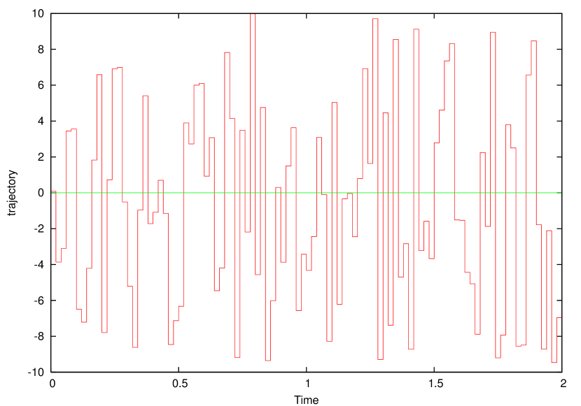
Figure 1: Example of a trajectory of a coarse grain independent process

Theorem 5

Given the system equations , $\dot{\bf x}_{t}={\bf f}({\bf x}_{t},t,{\bf\mbox{\boldmath$\xi$}}_{t}(\omega))$ note $\lambda_{f}({\bf x},t,\mbox{\boldmath$\xi$}_{t})$ the largest eigenvalue of the generalized Jacobian of ${\bf f}$ at time t according to some metric $M$.

A sufficient condition for the system to be coarse-grain contracting is that

• the random process $\lambda_{f}({\bf x},t,\mbox{\boldmath$\xi$}_{t})$ can be bounded independently from ${\bf x}$, ie there exists a stochastic process $\eta_{t}$ such that

  $$\forall{\bf x}\quad\lambda_{f}({\bf x}_{t},t,\mbox{\boldmath$\xi$}_{t})\leq\eta_{t}\qquad\mbox{a.s.}$$

• the process $\eta_{t}$ is a coarse-grain independent stochastic process with respect to a partition $(P_{n})$.

• We can uniformly bound the expectation of the $e^{\int_{P_{n}}\eta_{t}}$ with some $0\leq\eta<1$

  $$\forall n\quad\mathbb{E}((e^{\int_{P_{n}}\eta_{t}})^{2})\leq\eta$$

Proof 4

Proof.

$$\frac{1}{2}\ \frac{d}{dt}({\bf\delta{\bf z}}^{T}{\bf\delta{\bf z}})\leq\lambda_{f}({\bf x}_{t},t,\mbox{\boldmath$\xi$}_{t})\ {\bf\delta{\bf z}}^{T}{\bf\delta{\bf z}}\leq\eta_{t}\ \delta{\bf z}^{T}\delta{\bf z}\qquad\mbox{a.s.}$$

Which leads to

$$\|\delta{\bf z}\|\leq\|\delta{\bf z}_{0}\|\ e^{\int_{0}^{t}\eta_{t}dt}\qquad\mbox{a.s.}$$

Thus, we can define the system $Z_{n+1}=e^{\int_{t_{n}}^{t_{n+1}}\eta_{t}dt}Z_{n}$ and $Z_{0}=\|\delta{\bf z}_{0}\|$, which satisfies

$$\|\delta{\bf z}_{t_{n}}\|\leq Z_{n}$$

By definition of coarse-grain stochastic process and as $\mathbb{E}((e^{\int_{P_{n}}\eta_{t}})^{2})\leq\eta$, we can applied theorem 2 to conclude on the contraction in mean square of $Z_{n}$ with rate $\eta$

$$\mathbb{E}(\|{\bf\delta{\bf z}}_{t_{i}}\|^{2})\leq\mathbb{E}(Z_{i}^{2})\leq\|\delta{\bf z}_{0}\|^{2}\eta^{i}$$

$\square$

Remark 4

The condition imposed on the process $\eta_{t}$, namely $\mathbb{E}((e^{\int_{P_{n}}\eta_{t}})^{2})\leq\eta<1$, is really different from the condition we have seen for the almost sure contraction $\mathbb{E}(\eta_{t})\leq\eta<0$.

3 Part 2 : Noise’s dependency

Let us now turn on a very special case of perturbed systems, namely when the impact of the noise does not depend on the state space.

Proposition 1

Consider a contracting system $\dot{\bf\widehat{x}}={\bf f}({\bf\widehat{x}},t)$ and take a perturbed version of it $\dot{\bf x}_{t}={\bf f}({\bf x}_{t},t)+{\bf\mbox{\boldmath$\xi$}}_{t}(\omega)$. The system is automatically both contracting on average and almost surely contracting.

The proof is obvious as it is the case mention above of a system which is contracting for every $\omega$. Let us now study the mean and the variance of the unique solution.

3.1 Study of the average trajectory

Consider a contracting system $\dot{\bf\widehat{x}}={\bf f}({\bf\widehat{x}},t)$ in the metric $M=\mathnormal{I}$, take a perturbed version of it $\dot{\bf x}_{t}={\bf f}({\bf x}_{t},t)+{\bf\mbox{\boldmath$\xi$}}_{t}(\omega)$. Then, assuming that

• $\mathbb{E}(\mbox{\boldmath$\xi$}_{t})=0$

• $\forall t\ \|\mbox{\boldmath$\xi$}_{t}\|<\alpha$ almost surely with $\mathbb{E}(\alpha)<\infty$

we have that

$$\forall t\quad\mathbb{E}({\bf x}_{t})={\bf\widehat{x}}_{t}$$

Proof 5

Proof. Let ${\bf x_{\Delta}}={\bf\widehat{x}}-\mathbb{E}({\bf x}_{t})$ and consider

$${\bf x}_{\Delta}^{T}\frac{d}{dt}({\bf x}_{\Delta}) = {\bf x}_{\Delta}^{T}({\bf f}({\bf\widehat{x}},t)-\mathbb{E}({\bf f}({\bf x}_{t},t)))\quad\mbox{by dominated convergence theorem}$$

$$= {\bf x}_{\Delta}^{T}\mathbb{E}({\bf f}({\bf\widehat{x}},t)-{\bf f}({\bf x}_{t},t))$$

$$= {\bf x}_{\Delta}^{T}\mathbb{E}(\int_{0}^{1}\frac{\partial f}{\partial{\bf x}}({\bf\widehat{x}}+c{\bf x}_{\Delta},t)dc\ {\bf x_{\Delta}})$$

$$\leq \mathbb{E}(\int_{0}^{1}\lambda_{f}^{max}{\bf x}_{\Delta}^{T}{\bf x_{\Delta}})$$

$$= \lambda_{f}^{max}\|{\bf x}_{\Delta}\|^{2}$$

So we have that $\|{\bf x}_{\Delta}\|\leq\|{\bf x}_{\Delta_{0}}\|e^{2\lambda_{f}^{max}t}$. But $\|{\bf x}_{\Delta_{0}}\|=0$. $\square$

3.2 Study of deviation

Theorem 6

Take random system $\dot{\bf x}_{t}={\bf f}({\bf x}_{t},t)+{\mbox{\boldmath$\xi$}_{t}(\omega)}$ satisfying the conditions of the subsection 3.1. Suppose now that the deviations of the $\mbox{\boldmath$\xi$}_{t}$ are uniformly bounded

$$\mathbb{E}(\|\mbox{\boldmath$\xi$}_{t}\|)\leq\sigma$$

The deviation of ${\bf x}_{t}$ is then majored by the maximum deviation $\sigma$ in the following way:

$$\mathbb{E}(\|{\bf x_{1}}-{\bf x_{2}}\|)-\mathbb{E}(\|{\bf{\bf x_{1}}-{\bf x_{2}}}\|_{0})e^{\lambda_{f}^{max}\ t}\leq\frac{2\sigma}{|\lambda_{f}^{max}|}(1-e^{\lambda_{f}^{max}\ t}))$$

Proof 6

Proof. Let ${\bf\widetilde{x}}={\bf x_{1}}-{\bf x_{2}}$ Let us look at $\|{\bf\widetilde{x}}\|$

$$\left.\begin{array}[]{l}\dot{\bf x_{1}}={\bf f}({\bf x_{1}},t)+{\mbox{\boldmath$\xi$}_{1}}\\ \dot{\bf x_{2}}={\bf f}({\bf x_{2}},t)+{\mbox{\boldmath$\xi$}_{2}}\\ \end{array}\right\}\Rightarrow\frac{d}{dt}{\bf\widetilde{x}}=\int_{0}^{1}\frac{\partial f}{\partial{\bf x}}({\bf x_{2}}+c{\bf\widetilde{x}},t)dc\ {\bf\widetilde{x}}+{\mbox{\boldmath$\xi$}_{1}}-\mbox{\boldmath$\xi$}_{2}$$

Multiply by ${\bf\widetilde{x}^{T}}$, it becomes:

$${\bf\widetilde{x}^{T}}\frac{d}{dt}{\bf\widetilde{x}}={\bf\widetilde{x}^{T}}\int_{0}^{1}\frac{\partial f}{\partial{\bf x}}({\bf x_{2}}+c{\bf\widetilde{x}},t)dc\ {\bf\widetilde{x}}+{\bf\widetilde{x}^{T}}(\mbox{\boldmath$\xi$}_{1}-\mbox{\boldmath$\xi$}_{2})$$

$$\frac{1}{2}\frac{d}{dt}{\|\bf\widetilde{x}\|^{2}}\leq\lambda_{f}^{max}\|{\bf\widetilde{x}}\|^{2}+\|{\bf\widetilde{x}}\|\ \|\mbox{\boldmath$\xi$}_{1}-\mbox{\boldmath$\xi$}_{2}\|$$

So, by dominated convergence theorem again

$$\frac{d}{dt}\mathbb{E}(\|{\bf\widetilde{x}}\|)\leq\lambda_{f}^{max}\mathbb{E}(\|{\bf\widetilde{x}}\|)+\mathbb{E}(\|\mbox{\boldmath$\xi$}_{1}-\mbox{\boldmath$\xi$}_{2}\|)\leq\lambda_{f}^{max}\mathbb{E}(\|{\bf\widetilde{x}}\|)+2\sigma$$

Solving $\frac{d}{dt}\mathbb{E}(\|{\bf\widetilde{x}}\|)=\lambda_{f}^{max}\mathbb{E}(\|{\bf\widetilde{x}}\|)+2\sigma$ and using the positiveness of all terms in the equation (which means that replacing $=$ by $\leq$ just make the slope of increasement smaller), we have :

$$\mathbb{E}(\|{\bf\widetilde{x}}\|)-\mathbb{E}(\|{\bf\widetilde{x}}\|_{0})e^{\lambda_{f}^{max}\ t}\leq\frac{2\sigma}{|\lambda_{f}^{max}|}(1-e^{\lambda_{f}^{max}\ t}))$$

$\square$

3.3 Oscillator Synchronization

Consider two identical Van der Pol oscillators couples as

$$\ddot{\bf x}_{1}+\alpha({\bf x}_{1}^{2}-1)\dot{\bf x}_{1}+w^{2}{\bf x}_{1}=\alpha{\epsilon_{1}}(\dot{\bf x}_{2}-\dot{\bf x}_{1})$$

$$\ddot{\bf x}_{2}+\alpha({\bf x}_{2}^{2}-1)\dot{\bf x}_{2}+w^{2}{\bf x}_{2}=\alpha{\epsilon_{2}}(\dot{\bf x}_{1}-\dot{\bf x}_{2})$$

where

• $\alpha>0$, $w>0$

• $\epsilon_{1}$, $\epsilon_{2}$ are stationary processes

Using (Combescot, Slotine 2000), we can show that $x_{1}\xrightarrow[t\rightarrow\infty]{}x_{2}$ when

$$\mathbb{E}(\epsilon_{1})+\mathbb{E}(\epsilon_{2})>1$$

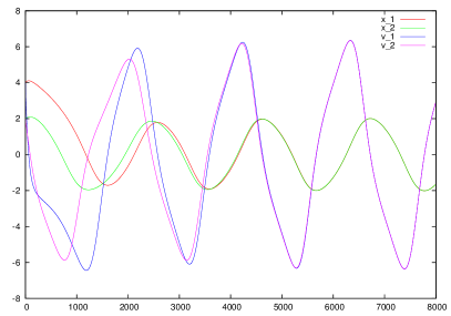
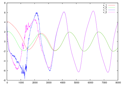
Figure 2: A comparison between stochastic synchronization of two Van der Pol oscillator with and without noise ($\epsilon_{1},\epsilon_{2}\in[-40,40]$)

Remark that we can add noise in the input of both oscillators, the synchronization still occurs on average (fig. 3).

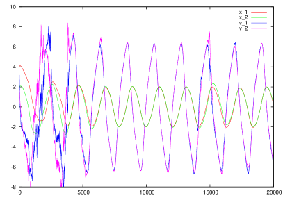
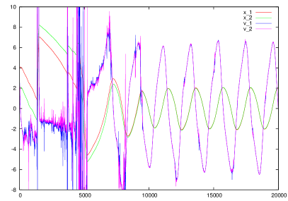
Figure 3: Stochastic synchronization with noise in input. Left part obtained with $\epsilon_{1},\epsilon_{2}\in[-80,80]$, right part with $\epsilon_{1},\epsilon_{2}\in[-400,400]$

References

• [Arnold, 1998] Arnold, L. (1998). Random Dynamical Systems. Springer-Verlag.
• [Jaswinski, 1970] Jaswinski, A. (1970). Stochastic Processes and Filterig Theory. Academic Press, New York.
• [Lohmiller and Slotine, 1998] Lohmiller, W. and Slotine, J. (1998). Contraction analysis for nonlinear systems. Automatica, 34(6):683–696.