A modeling approach to design a software sensor and analyze agronomical features - Application to sap flow and grape quality relationship

Abstract

This work proposes a framework using temporal data and domain knowledge in order to analyze complex agronomical features. The expertise is first formalized in an ontology, under the form of concepts and relationships between them, and then used in conjunction with raw data and mathematical models to design a software sensor. Next the software sensor outputs are put in relation to product quality, assessed by quantitative measurements. This requires the use of advanced data analysis methods, such as functional regression. The methodology is applied to a case study involving an experimental design in French vineyards. The temporal data consist of sap flow measurements, and the goal is to explain fruit quality (sugar concentration and weight), using vine’s water courses through the various vine phenological stages. The results are discussed, as well as the method genericity and robustness.

ampmtime

1 Introduction

In modern Agronomy, the recent progress of sensors provides a lot of data, among them many temporal data. This opens new challenges, such as the proper calibration of these sensors, and the use of temporal data to establish relationships with product characteristics and quality. These relationships are not easy to determine because of the high variability of biological material. This can be compensated by the integration of expertise, as Agronomy is a domain that has always relied as much on experience than on science. Nevertheless, for domain knowledge to be effectively used in collaboration with mathematical models and data, an expertise formalization step is required.

Our objective in this paper is to show the interest of a formalized data and knowledge-based approach to study a complex agronomical phenomenon, namely the influence of vine water deficit on grape quality.

Any index of vine water deficit aims at evaluating the amount of water effectively used by the vine in order to determine if if this amount falls short of some reference amount. Typically, the reference amount is the maximal amount of water a vine can use.

Various methods exist to characterize the level of water deficit experienced by the plant as reviewed by Jones (2004). Tissue water status can be assessed visually or by measurements of vine water potential. However, both methods have serious drawbacks. The lack of precision of visual observations often leads to yield reduction before visible symptoms occurs. The pressure chamber method used to measure water potential is slow and labour intensive, especially for predawn measurement, and is unsuitable for automation. In addition, measurements done with pressure chambers are very dependent on atmospheric conditions and vine phenological stage Olivo et al. (2009); Williams and Baeza (2007); Rodrigues et al. (2012); Santesteban et al. (2009).

Sap flow sensors, that indirectly measure changes in conductance, have recently become available. This sensitive measurement method requires a complex instrumentation and technical expertise for the definition of irrigation control thresholds Ginestar et al. (1998). The main advantages of sap flow method is to allow automatic and continuous measurement of water flowing through the plant, which is directly related to transpiration Escalona et al. (2002); Jones (2004); Cifre et al. (2005); Zhang et al. (2011).

However, sap flow is a complex phenomenon and expert knowledge is necessary to convert raw data into useful transformed data, i.e. water courses, by designing a software sensor. Once these data transformations are validated, it opens the way to a range of new studies, based on vine’s water courses.

In this paper, we will first show how a formalized data and knowledge-based approach can be useful to design a software sensor. Knowledge formalization will be done by using ontologies, which take increasing importance in the field of Life Sciences Villanueva-Rosales and Dumontier (2008); Thomopoulos et al. (2013), for their ability to model and structure qualitative domain knowledge.

In a second step, water use trajectories will be put in relation to grape quality indicators such as Berry Weight or Sugar Concentration, using recent data analysis tools and formalized knowledge. Innovative data analysis tools include functional data analysis that offers the possibility to use curve (functional) data instead of scalar data. Functional data analysis has not been much used in life sciences yet Ullah and Finch (2013), though it could be of particular interest in the Vine and Wine Industry, and more generally for modern Agronomy.

The modeling task is divided into two independent parts: software sensor design and temporal data analysis. If the sensor design procedure were different, this would not affect the validity of the data analysis methodology.

The methodological work is illustrated by a case study, involving an experimental design on several vineyards in the Languedoc region (France).

The paper is organized as follows: Section 2 presents the material and methods. It is divided into four parts. The first part gives some elements about data and the second one presents ontology-based formalization. The software sensor design, that relies on the use of mathematical models, data and formalized knowledge, is described in the third part. The selected example shows how it is possible to transform raw sap flow data into vine water deficit courses. The fourth part describes the methods used for analysing the sofware sensor output in relation to product quality. Section 3 presents and discusses the results and their relationship with grape composition (Sugar Concentration, Berry Weight). Some concluding remarks are given in Section 4.

2 Material and methods

In this section, we propose to follow four steps:

• to describe the experimental design with its input and output variables

• to formalize eco-physiological knowledge using an ontology

• to design a software sensor using formalised knowledge, a mathematical model, and data

• to relate software sensor output to product quality using decision trees and functional analysis.

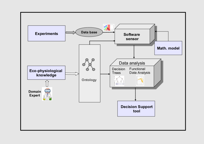
Figure 1: Outline of the proposed modeling approach.

Expert knowledge plays an essential part in the modeling process, and we focus on providing an efficient way to separate the data-based statistical procedures from the qualitative knowledge-based assumptions.

The outline of the approach is given in Fig.1. Experiments feed a data base. The software sensor integrates data from the data base, an ontology and a mathematical model. Its outputs can be analyzed using data analysis. This analysis also calls for eco-physiological knowledge, essentially about the phenological stages. Therefore, the ontology is used at two different levels: software sensor design and data analysis supervision. Data analysis is performed on the basis of two complementary perspectives for determining relations between software sensor temporal output and product quality. The first line of work is to design scalar explanatory variables, by summarizing a period of interest in compliance with the eco-physiological knowledge. These variables can then be used as input to decision trees. The second line of work is to use recent advances in functional data analysis, so that the inputs to the statistical model are the temporal data as a whole.

In the following, the approach is illustrated with a software sensor to estimate vine water courses and their relation to grape quality. Nevertheless, the proposed methodology is generic in many aspects, and could be useful in the development of other decision support tools in Agronomy, provided that expertise and temporal data are available.

2.1 Experimental design

Data used in this paper come from a multi-site experiment located in the south of France. The same experimental design was set up in seven sites across the Languedoc Roussillon region in order to test for the effects of vine stress status on grape potential and wine quality in contrasted environmental conditions. In total, vine water stress status was followed over 16 vine plots, each planted with one of the following varieties: Merlot, Cabernet-Sauvignon, Grenache or Chardonnay.

To get a wider range of vine water statuses during the season, an irrigation treatment was applied for two years on each of the eight site-variety combinations. The irrigation treatment consisted of two modalities, replicated twice, yielding 32 experimental subplots. In the non irrigated subplots, vines only received natural precipitations during the growing season while in the irrigated subplots, vines received regular extra-amounts of water through drippers line (emission rate from 2 to 4 $\mathrm{l}\ \reciprocal\mathrm{h}$, 1 to 2 drippers per plant).

Several kinds of data, collected according to an experimental design are available: local meteorological data, vine water stress related measurements, phenological state assessments, as well as grape quality analyses.

2.1.1 Meteorological data

Hourly meteorological data on windspeed ($\mathrm{k}\mathrm{m}\ \reciprocal\mathrm{h}$), minimal, maximal and mean air temperature ($\mathrm{\SIUnitSymbolCelsius}$), air humidity (%), solar radiation ($\mathrm{W}\ \mathrm{m}\rpsquared$) and amounts of precipitations ($\mathrm{m}\mathrm{m}$) were extracted from local meteorological stations for each site.

Transformed data

Hourly vapor pressure deficit ($\mathit{VPD}$) and reference atmospheric evaporative demand (potential evapotranspiration, $\mathit{ET}_{ref}$) were calculated according to methodologies referred to as FAO-56 Allen et al. (1998). Calculation of reference atmospheric evaporative demand ($\mathit{ET}_{ref}$ in $\mathrm{m}\mathrm{m}\ \reciprocal\dday$) is based on Penman-Monteith formula.

Daily meteorological data were obtained from hourly data after a trapeze integration. Thermal time, i.e. the accumulation of growing degree days (GDD) from April 1^st was calculated by daily integration of mean air temperature minus a base temperature of 10 $\mathrm{\SIUnitSymbolCelsius}$ which is considered as the simplest model to estimate vine phenology Parker et al. (2011).

2.1.2 Phenological data

The main phenological phases (budbreak, bloom, nouaison, veraison) were estimated visually in each experimental plot when 50% of the plants reached the stage. Bloom was observed when 50% of the clusters had the cap off. Nouaison was defined using the bloom stage, according to local expert knowledge (see Section 2.2.1).Veraison dates were recorded when 50% of the fruit had turned red.

2.1.3 Vine water status data

Vine water status was monitored by two kinds of measurements: discrete measurements of leaf water potential at predawn ($\Psi_{b}$, or predawn LWP) and continuous measurements of sap flow.

Leaf water potential at predawn

LWP measurements were conducted every week from the end of June to the end of August with a pressure chamber at predawn (between $\approx$ 3.00 am and $\approx$ 5.00 am).

Sap flow

The energy balance method (Sakuratani, 1981) was used to measure sap flow with Sap IP system (Dynamax, Houston, TX, USA). There is one variety per vineyard site. The vineyard site is divided into 2 irrigation treatments. Two vineyard rows were selected. One row represents one irrigation treatment. In each selected row, 2 vines were equipped with one sensor. Each sensor measured vine sap flow rate every 15 minutes. The 2 selected vines were within 25 meters of each other within the same row.

Sap flow rates measured on each vine were averaged on an hourly basis within each row. Total sap flow of each vine was calculated as the product of sap flux density and cross sectional sap wood area at the point of measurement. Various expert methods were applied to filter out nighttime, weak and erroneous signals. Sap flow measurements were scaled at the plant level according to plant leaf area estimates corresponding to each sensor. The daily sap flow assumed to measure daily vine transpiration was computed by adding all hourly sap flow rates measured during the day. The volumetric flux per vine ($\mathrm{g}.\reciprocal\mathrm{h}$) was converted into $\mathrm{m}\mathrm{m}.\reciprocal\mathrm{h}$ taking into account the respective area of ground per vine. Daily vine transpiration will be noted $T(t)$.

2.1.4 Fruit composition quality data

Starting two weeks before harvest, fruit was sampled for each irrigation treatment in each vineyard. Fruit data was collected at three different dates. Fruit composition analysis focused on berry weight ($\mathrm{g}$), sugar concentration ($\mathrm{g}\ \reciprocal\mathrm{l}$), acidity ($\mathrm{g}$H2SO4$\ \reciprocal\mathrm{l}$), anthocyanes and assimilable nitrogen ($\mathrm{m}\mathrm{g}\ \reciprocal\mathrm{l}$).

2.2 Formalizing knowledge

In this section, our aim is to show how ontologies can be used to formalize domain knowledge and to design a software sensor.

In information science, an ontology formally represents knowledge as a set of concepts within a domain, and the relationships between pairs of concepts.

Ontologies are becoming increasingly popular, due to the great amount of available (complex) data and to the need for modeling (qualitative) knowledge and structural information. This need first arose out of the development of the World Wide Web. However, there are still very few attempts to combine ontologies and statistical or data-driven models. This could be particularly useful in Life Sciences and Agronomy Villanueva-Rosales and Dumontier (2008); Thomopoulos et al. (2013); Destercke et al. (2013).

The main incentives for using ontologies Guarino et al. (2009) are the following ones:

1. To share a common understanding of structured information Musen (1992);

2. To explicit the specificities of domain knowledge;

3. To identify ambiguous or inappropriate model choices.

For the present work, a specfic ontology has been built, in order to formalize the concepts and relations required to design a vine water deficit indicator and to analyze its impact on grape quality.

The general class diagram of the ontology, called Ontology of Vine Water Stress (OVWS), is shown on Figure 2 as a Unified Model Language (UML) diagram. It is composed of concepts, represented as rectangular boxes, and of relations, represented by arrows. Formally, the ontology $\Omega$ is defined as a tuple $\Omega=\{\mathcal{C},\mathcal{R}\}$ where $\mathcal{C}$ is a set of concepts and $\mathcal{R}$ is a set of relations.

Let us comment the main concepts and relations.

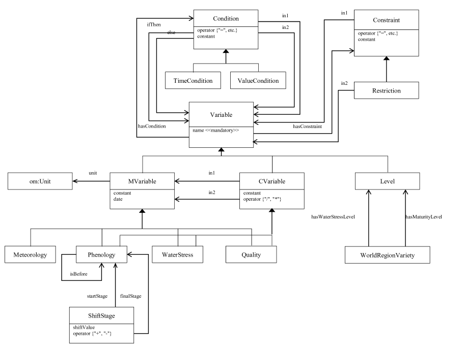
Figure 2: Class diagram of the ontology of Vine Water Stress

2.2.1 Concepts

In this ontology, four kinds of primary concepts were defined: Variable, Condition, Constraint and ShiftStage. All other concepts are subconcepts of these primary ones and linked to them by a subsumption relation, as explained in Section 2.2.2. For instance, in Figure 2, $Meteorology$, $Phenology$, WaterStress and $Quality$ are subconcepts of Variable.

• All variables must have a name, they can have a date, a unit and a default value. The units are taken from $\mathit{OM}$, an ontology of units of measures and related concepts Rijgersberg et al. (2013). .

• The Condition concept is defined with a comparison operator and two operands. It will be used together with the hasCondition (${\mathcal{HCO}}_{c}$) relation, defined in Section 2.2.2.

• The Constraint concept is defined with a comparison operator and one operand. It will be used together with the hasConstraint (${\mathcal{HCS}}_{c}$) relation, defined in Section 2.2.2. The Restriction concept is a subconcept of Constraint, and is a specific two-fold constraint.

• The ShiftStage concept is proposed in order to determine a phenological stage from another one. This is the case for the $Nouaison$ stage, which is not generally observed. Its date can be estimated by shifting the $Bloom$ date by $k$ $GDD$, where $k$ can be variety-dependent. $Nouaison$ and $Bloom$ are instances of the $Phenology$ concept.

2.2.2 Relations

On Fig. 2, there are two kinds of arrows: regular arrows and thick-headed ones. The former correspond to the subsumption relation, and the latter to the other relations. In that last case, the arrow label gives the relation name, for instance hasCondition.

• The subsumption relation, also called the ‘kind of’ relation and denoted by ${\preceq}$, defines a partial order over $\mathcal{C}$. Given a concept $c\in{\mathcal{C}}$, we denote by ${\mathcal{C}}_{c}$ the set of sub-concepts of $c$, such that:

  $${\mathcal{C}}_{c}={\{c^{\prime}\in{\mathcal{C}}|c^{\prime}{\preceq}c\}}.$$ (1)

  For example, in Figure 2, let us consider the concept $c=\textit{Variable}$. We have ${\mathcal{C}}_{\text{Variable}}=\{\textit{MVariable},\textit{CVariable},\textit{Level}\}$, where MVariable represents a measurement available in a data base, CVariable a variable calculated following a given method, and Level a constant value depending on some other concepts.

• The subsumption relation can be multiple. For instance a $Phenological$ $concept$ can be such as $c{\preceq}CVariable$ or $c{\preceq}MVariable$.

• The $\mathit{isBefore}$ relation allows to represent temporal precedency. It is very important for checking the consistency of the phenological stage dates, where $bloom$ has to occur before $veraison$, and so on.

• The HasCondition (${\mathcal{HCO}}_{c}$) relation, where $c$ represents the concept on which the condition is to be applied, is used together with a condition.

• Similarly, the HasConstraint (${\mathcal{HCS}}_{c}$) relation allows the application of a $constraint$ on the $c$ concept.

Examples of use will be given in Section 2.3.2.

The ontology is modelled using the Web Ontology Language (OWL). OWL is a semantic markup language for publishing and sharing ontologies on the World Wide Web, which is specified using W3C recommendations. The use of OWL allows reusing ontologies developed elsewhere, such as OM.

Note that each modeling component: data base, ontology and mathematical modelling or data analysis, can be modelled independently, using its favorite language (sql, R, OWL). The communication between the various components can be implemented by a high level interface, written in Python, PHP or Java.

2.3 Design of the software sensor for vine water stress estimation

Based on the knowledge formalized in the ontology given in Fig.2 and on a mathematical model Ferreira et al. (2012), the software sensor is designed to transform the calibrated transpiration measurements from sap flow sensors into a vine water deficit estimator, denoted by $\mathit{Ks(t)}$.

The different steps of the methodology used to design $\mathit{Ks}$ are summarized in Fig.3 and detailed in the following subsections.

2.3.1 Sap flow under limiting soil water condition : computation of $\mathit{Ks}$

$\mathit{Ks}$ is the ratio between actual and maximum crop transpiration, defined as:

$$\mathit{Ks(t)}=\frac{T(t)}{\mathit{T_{max}(t)}}$$ (2)

It accounts for the decline in vine water use due to soil moisture deficit. Even if some authors Allen et al. (1998) present a general proposal for estimating $\mathit{Ks}$, specific $\mathit{Ks}$ functions for vineyards, from field experiments, are not generally available.

In the vine context, in Eq.2, $T$ is the daily measured transpiration from sap flow and $\mathit{T_{max}}$ is the daily maximal vine transpiration obtained under dry soil condition (meaning no cover crop) when soil moisture is non limiting, defined as in Allen et al. (1998).

$$T_{max}(t)={Kc_{B}}(t)\ {ET}_{ref}(t)$$ (3)

$\mathit{ET_{ref}}$ is the reference evapotranspiration and $\mathit{Kc_{B}}$ a coefficient linearly related to the leaf area index (LAI) or to the fraction of ground coverage Williams and Ayars (2005); Picón-Toro et al. (2012). As $\mathit{Kc_{B}}$ is dependent upon crop type and management practices, which will influence the rate of canopy development and the ultimate canopy size, i.e. amount of ground cover (Allen et al. (1998)), a site-specific determination of $\mathit{Kc_{B}}$ is necessary for each vineyard.

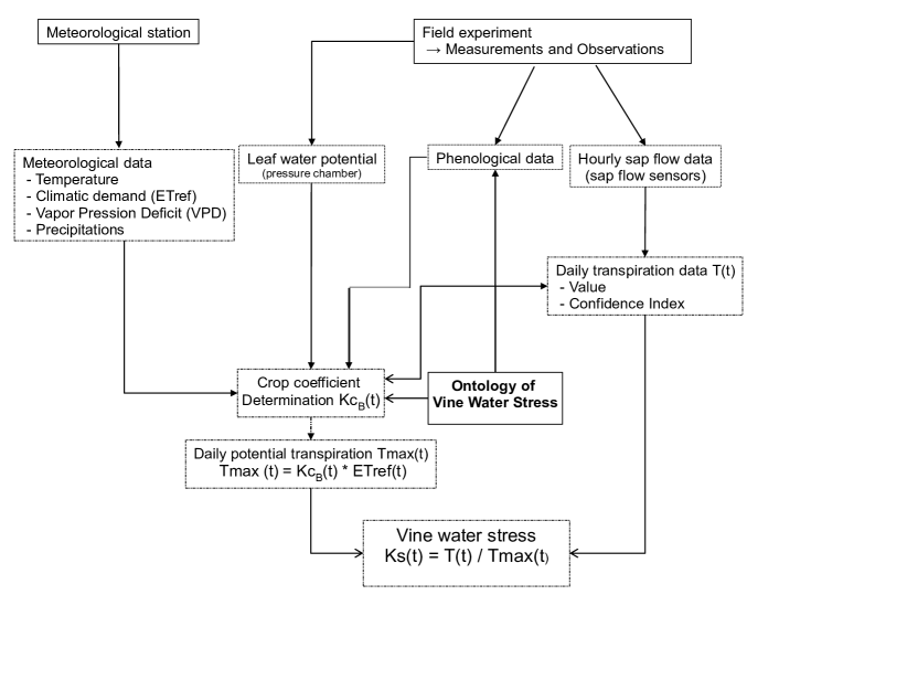
Figure 3: Methodological steps for the vine water deficit ($\mathit{Ks}$) estimation.

2.3.2 Sap flow under non limiting soil water condition : computation of dry soil $Kc_{B}$

No direct measurements are available to determine $\mathit{Kc_{B}}(t)$ (see Eq.3), which is vine specific and varies with leaf area. We propose to use formalized concepts and relations based on expertise, all of them implemented in the OVWS ontology. $\mathit{Kc_{B}}$ profile is divided into two growth stages : $\mathit{L_{dev}}$ and $\mathit{L_{mid}}$ as presented in Fig.4. To determine $Kc_{B}(t)$, two hypotheses on the curve shape are assumed:

$$\mathit{Kc_{B}}(t)=f(t)\mbox{ for }t<t_{K^{*}}$$ (4)

$$\mathit{Kc_{B}}(t)=K^{*}\mbox{ for }t\geq t_{K^{*}}$$ (5)

where $f(t)$ is assumed to be linear in $t$, and $t_{K^{*}}$ is the breakpoint for which $Kc_{B}$ reaches the plateau $K^{*}$.

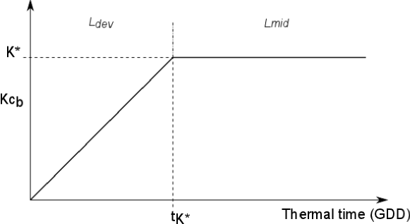
Figure 4: Theoretical curve of $Kc_{B}$ evolution during the season.

The key point is to set $t_{K^{*}}$, or indifferently $\mathit{K^{*}}$. According to Eq.3, we make the hypothesis that, in the absence of water deficit, $\mathit{K^{*}}$ is defined as:

$$\mathit{K^{*}}=\frac{\mathit{T}(t_{K^{*}})}{\mathit{ET}_{ref}(t_{K^{*}})}$$ (6)

Using the OVWS ontology defined in Section 2.2, the following rules are set up to automatically define a limited number of potential options for $t_{K^{*}}$. The interest of having the rules and concepts defined in an ontology is two-fold: $i)$they have to be completely explicit, $ii)$they can evolve independently of the numerical procedures.

1. Selection based on phenology

   A linear relationship exists between $\mathit{Kc_{B}}$ variations and leaf area index (LAI) or the fraction of ground covered by the vine Ferreira et al. (2012). We thus assume that peak $\mathit{Kc_{B}}$ (i.e. $\mathit{K^{*}}$) is reached when LAI stops increasing. Consequently, the search period for $\mathit{K^{*}}$ has been limited to the period between budbreak and veraison.

   These two concepts are defined as subconcepts of the Phenology concept, itself being a subconcept of MVariable. The period limitation is intanciated by two TimeConditions, applied onto the $\mathit{Kc_{B}}{\preceq}CVariable$ concept, the ${\mathcal{HCO}}_{c}$ relation where the $Condition$ is characterized by a comparison operator $\leq$ (resp. $\geq$) and the Veraison (resp. Budbreak) concept.

2. Selection based on predawn leaf water potential

   Conditions of maximal soil moisture availability could be inferred from predawn leaf water potential measurements, associated with a confidence interval derived from VPD. A rule was set so that $\mathit{K^{*}}$ has to be reached before the first day at which predawn LWP measurement reveals a water stress. The levels to which predawn LWP characterises water stress can be defined by the stakeholder, or else set in agreement with a standard level, based on a region or/and variety.
   This is implemented in the ontology by the WorldregionVariety and level ${\preceq}Variable$ concepts.

3. Selection based on meteorology

   Transpiration measurement through sap flow is sensitive to climatic conditions, mainly light and $\mathit{VPD}$. To account for sensitivity of transpiration measurements to $\mathit{VPD}(t)$, a filtering rule was set to remove computed $Kc_{B}(t)$ obtained in situations of heat spikes, defined as period with $\mathit{VPD}$ greater than a given level, set to 3.5 $\mathrm{k}\mathrm{Pa}$ in the present case study.
   The rule is implemented using a ${\mathcal{HCS}}_{c}$ relation, applied onto the
   $\mathit{Kc_{B}}{\preceq}CVariable$ concept, where the $Constraint$ is characterized by a comparison operator $\leq$ and the $\mathit{VPD}{\preceq}Meteorology{\preceq}MVariable$ concept.

4. Selection based on curve shape

   By definition, $\mathit{K^{*}}$ is reached when the ratio $\displaystyle\frac{\mathit{T}(t)}{\mathit{ET_{ref}(t)}}$ reaches a maximum during a few days (as $T(t)$=$T_{max}(t)$ and $Kc_{B}(t)$=$K^{*}$) and then decreases (as $T(t)$<$T_{max}(t)$ due to limiting soil water conditions while $Kc_{B}(t)$=$K^{*}$). As such, potential options for $t_{K^{*}}$ have been defined at points with a null first derivative and a negative second derivative.
   This selection is implemented using two concepts: $\dot{\mathit{K^{*}}}$ and $\ddot{\mathit{K^{*}}}$, both such as ${\preceq}WaterStress{\preceq}CVariable$ , and a ${\mathcal{HCS}}_{c}$ relation with a
   $Constraint$ characterized by a comparison operator $\leq\epsilon$ or $\leq 0$.

User selection based on expert knowledge

The analysis of $\displaystyle\frac{\mathit{T}(t)}{\mathit{ET}_{ref}(t)}$ curve shape, associated with all previous rules based on phenology, meteorology and predawn leaf water potential leads to the proposal of a small finite set of $\mathit{t_{K^{*}}}$ candidates.

The final choice is left to the stakeholder who is the best aware of the management practices or particular uncontrolled events that could have interfered with vine growth (irrigation, leaf removal, treillis system, …) and therefore $\mathit{Kc_{B}}$ curve.

2.4 Relating software sensor output to product quality

The software sensor output consists of temporal data, and various methods can be used to study the relationships between these data and product quality. Two complementary lines of work, based on statistical methods, are explored in the present work. The first one consists of extracting significant scalar parameters from the temporal data and using them as input to decision trees, in order to provide the most discriminant features. The second one uses functional data analysis, that gives the possibility to model the temporal data impact on product quality as a whole. However, curve analysis is a recent research topic, with relatively few methods available, in comparison with classical data analyses.

This section is divided into three parts. The first part describes how to use the formalized knowledge for extracting significant scalar parameters from the temporal data. The other two parts give some elements necessary to understand the statistical methods that will be used: decision trees and functional analysis.

2.4.1 Extracting scalar parameters from software sensor output

Meaningful scalar parameters can be extracted from temporal courses determined by the software sensor outputs. In many cases, expert knowledge can be the support of such extraction procedures. In the case of vine water courses, this can be achieved by taking into account important phenological periods, which are defined as concepts in the ontology (see Fig.2).

Three periods were first defined according to phenological stages: the whole season, the pre-veraison period, which goes from the nouaison stage to the veraison stage, and the post-veraison period which ranges from the veraison stage to the harvest date. In a second step, the post-veraison period was divided by taking into account the maturity stage of berries (see Section 2.1.2), which allowed to a add a fourth period ranging from veraison to maturity. Maturity stage is reached when the ratio between Sugar Concentration and acidity in grapes yields a given threshold, defined according to variety

Using trapeze integration under $\mathit{Ks}$ curves over these four periods, the continuous $\mathit{Ks(t)}$ curve was summarized into four new variables corresponding to the cumulative amount of stress encountered by the vine over these periods: NouHarv, NouVer, VerHarv and VerMat. Table 1 gives the summary of these four aggregated variables for each plot. Since all these aggregated variables are based on the area under the curve, the lower their value, the stronger the water stress over the considered period.

Site	Variety	Irrigation	NouHarv	NouVer	VerHarv	VerMat
LB-CS	Cabernet-S.	$i_{0}$	1165.6	704.6	432.6	432.6
		$i_{1}$	1117.8	713.8	375.0	347.6
OUV-Mer	Merlot	$i_{0}$	742.1	457.2	278.3	163.9
		$i_{1}$	1233.8	814.7	403.4	247.9
StGER-Mer	Merlot	$i_{0}$	608.9	470.9	131.6	129.4
		$i_{1}$	808.3	473.4	327.0	214.5
PR-Mer	Merlot	$i_{0}$	655.4	381.8	250.2	199.5
		$i_{1}$	722.7	398.3	313.4	266.2
StSAU-Char	Chardonnay	$i_{0}$	695.3	442.6	241.9	213.6
		$i_{1}$	693.8	414.0	265.3	253.7
RIE-Gre-Chm	Grenache	$i_{0}$	651.1	465.2	169.9	169.9
		$i_{1}$	620.0	390.9	209.5	209.5
RIE-Gre-Chp	Grenache	$i_{0}$	512.3	380.0	123.0	NA
		$i_{1}$	963.9	580.2	362.0	362.0
PIO-Gre	Grenache	$i_{0}$	677.2	458.4	212.0	152.3
		$i_{1}$	887.4	514.4	363.8	180.8

Table 1: Values of aggregated variables for each site-variety-irrigation treatment combination (i) over the entire season NouHarv, (ii) before veraison NouVer, (iii) after veraison VerHarv and (iv) from veraison to maturity VerMat.

2.4.2 Decision trees as interpretable models

Decision tree algorithms are well established learning methods in supervised data mining and statistical multivariate analysis. They allow to display non linear relationships between features and their impact on a response variable, in a compact way. A low complexity Ben-David and Sterling (2006) is essential for the model to be interpretable, as confirmed by Miller’s conclusions Miller (1956) relative to the magical number seven.

Decision trees can handle classification problems or regression cases, depending on the nature of the response variable. We present here the regression case, where the response variable is numerical.

Input to regression decision trees consists of a collection of $N$ training cases, each having a tuple of values for a set of $P$ input variables, and one output variable $(\mathbf{x_{i},y_{i}})=(x_{1,i},x_{2,i}\ldots x_{P,i},y_{i}).$ An input $X_{p}$ ($p=1...P$) is continuous or discrete and takes its values $(x_{p,i})_{i=1\dots N}$ on a domain $\mathcal{X}_{p}$. The goal is to learn from the training cases a recursive structure (taking the shape of a rooted tree) consisting of (i) leaf nodes labeled with a mean value and a standard deviation, and (ii) test nodes (each one associated to a given variable) that can have two or more outcomes, each of these linked to a subtree.

Decision trees are easily interpretable for a non-expert in statistical or learning methods, and facilitate exchanges with the domain expert.

Well-known drawbacks of decision trees are the sensitivity to outliers and the risk of overfitting. To avoid overfitting, cross-validation is included in the procedure and to gain in robustness, a pruning step usually follows the tree growing step (see Quinlan (1986); Breiman et al. (1984); Quinlan (1993)).

Note that the CART family Breiman et al. (1984), based on binary splits. is mostly used by statisticians. There is another tree family Quinlan (1986), called ID3 Quinlan (1993), allowing non binary splits and mostly used by artificial intelligence researchers.

In this work, we used CART-based trees. In that case, the splitting criterion is based on finding the one predictor variable (and a given threshold of that variable) that results in the greatest change in explained deviance (for Gaussian error, this is equivalent to maximizing the between-group sum of squares, as in an ANOVA). This is done using an exhaustive search of all possible threshold values for each predictor. The implementation used for decision trees is the R Development Core Team (2009) software with the rpart package. Specifying variety, NouVer, VerHarv and VerMat as explanatory variables, we computed decision trees on maximum values of grape quality features over the season.

2.4.3 Functional data analysis

Functional linear regression is an approach to model the relationship between a scalar dependent variable $Y$ and a functional predictor $X(t)$, a function of a real variable $t$ (time for example). The model is written as

$$Y_{i}=\beta_{0}+\int X_{i}(t)\beta(t)dt+\varepsilon_{i}\,,\quad i=1,\dots,n$$ (7)

where $\varepsilon_{i}$ is a random error, $\beta_{0}$ is the intercept of the model and $\beta(t)$ is the coefficient function, both unknown and to be estimated from independent observations $(X_{i}(t),Y_{i})_{i=1,\dots,n}$. In this model, $\beta(t)$ determines the effect of $X_{i}(t)$ on $Y_{i}$. For example, $X_{i}(t)$ has a greater effect on $Y_{i}$ over regions of $t$ where $|\beta(t)|$ is large. On the opposite, $X_{i}(t)$ has no effect on $Y_{i}$ over regions of $t$ where $\beta(t)$ is zero. Estimating $\beta(t)$ in model (7) has given rise to an increasing litterature during this last decade, see for example Ramsay and Silverman (2005). A common approach involves projecting $\beta$ and the $X_{i}$’s in a $p$-dimensional basis function where $p$ is large enough to capture the unknown variations of $\beta$, but small enough to regularize the fit.

Interpretation of such estimators is not that easy. Recently, James et al. (2009) introduced new estimators that are both interpretable, flexible and accurate. The method, called “Functional Linear Regression That’s Interpretable” (FLRTI), is based on a particular basis function and model selection principles. The $\beta$ function is either assumed to be zero or to have a simple linear form. The reason behind the first assumption is that the $X_{i}(t)$ observations are not of equal importance to explain the response $Y_{i}$. As said above, $X_{i}(t)$ has no effect on $Y_{i}$ when $\beta(t)=0$. The second assumption is made for technical reasons to simplify the model. All together, this model will have a high explanatory capability, contrary to a pure predictive model. These assumptions will constraint the estimation of the regression model (7), which corresponds to a penalized regression in sparse models. Two tuning parameters have to be fixed, a penalty term $\sigma$ and a weight $\omega$. The penalty term is part of the model selection process (by lasso or Dantzig selector). The largest the $\sigma$, the more the form-related constraint is enforced. The weight $\omega$ impacts the relative number of zeros of the $\beta$ function. A weight of 0 indicates that only the linear form constraint is respected.

The FLRTI method is implemented in an R function available on J. Gareths’s web page. A cross-validation algorithm is also proposed to optimize the choice of $\sigma$ and $\omega$.

Using the FLRTI method, we analysed the effects of water stress curve over the season ($\mathit{Ks(t)}$) on Berry Weight and Berry Sugar Concentration at harvest.

3 Results

In this section, we first present the results of the $\mathit{Ks(t)}$ estimation using the software sensor. In a second step, we study the relationship between $\mathit{Ks(t)}$ and grape quality features, using the methods described in Section 2. In the following, we will refer to irrigated treatments with $i_{1}$, and to non irrigated ones with $i_{0}$.

3.1 Vine water stress course $\mathit{Ks(t)}$ estimation

Sap flow data require a pre-treatment, including sensor selection and signal smoothing. Sap flow sensors have only been used recently in European vineyards. Thus, calibration protocols are not established yet and therefore sensors can still be unreliable. Consequently, a selection step is required.

Sensor reliability has been assessed on the basis of the number of incorrect hourly measurements resulting from expert filtering methods. A sensor was considered reliable when less than 5% of the hourly data were filtered out. For each variety-irrigation combination, the mean daily vine transpiration was calculated as the mean of daily measures from reliable sensors, which helped limiting the variability in plant transpiration measurements. However, one of the major drawback of sensor selection was the potential lack of reliable measurements on a daily basis.

To capture important patterns in daily sap flow data, while leaving out noise and extreme variations (daily peak), sap flow courses were smoothed with the central moving average method with a five day window. This smoothing allowed the removal of missing values and extreme peaks.

3.1.1 $K^{*}$ determination

Regarding all site-variety combinations, the knowledge-based algorithm for $t_{K^{*}}$ determination proposed from 5 to 9 candidates (resp. from 4 to 8 candidates) in the non-irrigated $i_{0}$ (resp. irrigated $i_{1}$) treatments. Most of the dates proposed by the mathematical algorithm were in accordance with expert knowledge, so allowing the expert to choose $t_{K^{*}}$ within the algorithm suggestions (Fig.5). The results are given in Table 2.

Site	Variety	Irrigation	$K^{*}$	$t_{K^{*}}$ (GDD)	First irrigation(GDD)
La Baume	CS	i0	20.3	677.9
		i1	32	698.6	1268.3
Pech Rouge	Merlot	i0	19.4	614.5
		i1	26,6	614.5	610.4
St Gervasy	Merlot	i0	69.3	625.3
		i1	85.1	669.4	844
Ouveillan	Merlot	i0	37.1	829.2
		i1	21	1005.1	939.7
Piolenc	Grenache	i0	44.3	530.1
		i1	58.1	530.1	864.4
Rieux	Grenache+	i0	43.4	600.5
		i1	29.1	594.5	789.5
Rieux	Grenache-	i0	29.2	580
		i1	46.1	580	789.5
St Sauveur	Chardonnay	i0	43.3	642
		i1	54.4	749.7	777.2

Table 2: Values of basal crop coefficients $K^{*}$ and dates ($t_{K^{*}}$ in GDD) at which they were estimated in the site-variety-irrigation treatment combinations during season 2012.

Fig.5 illustrates the results for the Grenache variety at the Piolenc site.

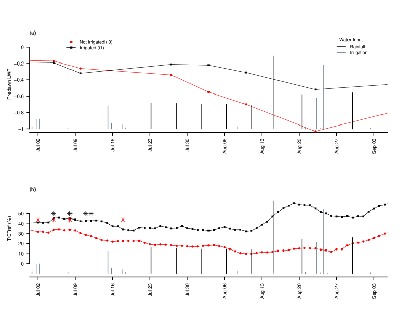
Figure 5: (a) Vine water status as indicated by leaf water potential and (b) determination of $K^{*}$ and $t_{K^{*}}$ (stars) based on expert knowledge following the mathematical algorithm suggestions for non irrigated (red bullets) and irrigated (black squares) treatments on the Grenache variey at Piolenc site.

The validity of the $K^{*}$ determination procedure can be assessed according to different points. First, the results regarding $K^{*}$ determination based on the coupling of mathematical algorithms and expert knowledge were consistent with existing literature. Indeed, most of $t_{K^{*}}$ occurred between 600 and 700 GDD after budbreak (Table 2), which is in accordance with $t_{K^{*}}$ reported in Picón-Toro et al. (2012) from a 3 year study in western Spain on Tempranillo, and in FAO-56 Allen et al. (1998), that respectively reported $t_{K^{*}}$ around 650 GDD and 555-592 GDD after budbreak.

3.1.2 Maximal transpiration and $\mathit{Ks}$ estimation

Following determination of $K^{*}$ and $t_{K^{*}}$, $Kc_{B}(t)$ was calculated over all $t$ values (Eq.4). Its evolution for a Grenache variety is plotted on Fig.6, both in calendar time (a) and thermal time since budbreak (b).

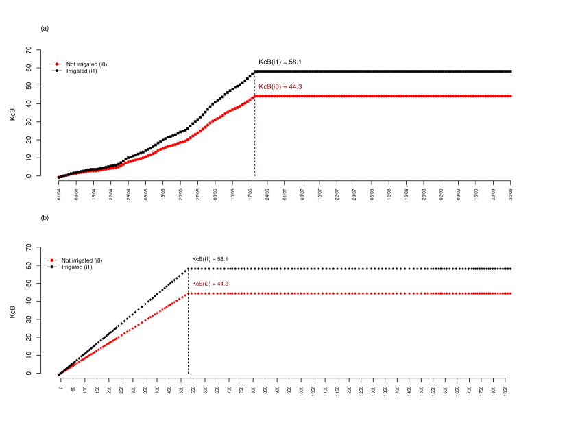
Figure 6: Evolution of vine basal crop coefficient ($Kc_{B}$) during the season at Piolenc site with Grenache variety, from budbreak to harvest. (a) x-scale in Julian days - (b) x-scale in GDD since budbreak.

$Kc_{B}(t)$ was then used to calculate the daily vine maximal transpiration ($\mathit{T_{max}}$), according to Eq.3. Finally, $\mathit{Ks(t)}$ was calculated as the daily ratio of measured transpiration by reliable sensors over potential transpiration (Eq.2).

Figure 7 shows vine water status according to both indicators: (a) Predawn LWP and (b) $\mathit{Ks}$ during the season 2012 in a Grenache variety of the Languedoc-Roussillon region.

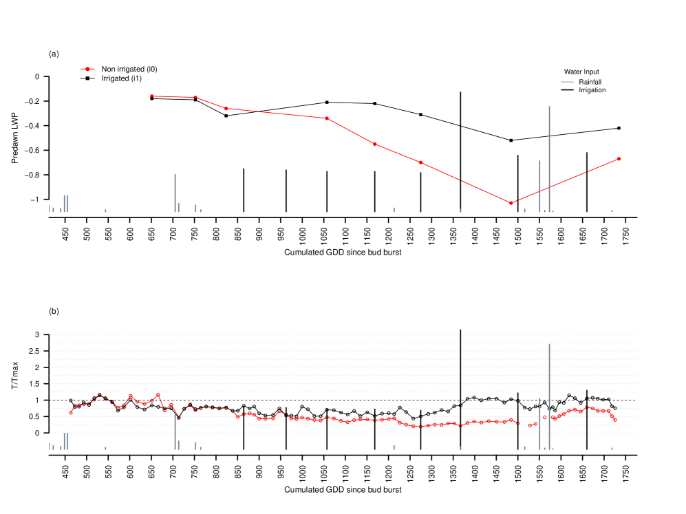
Figure 7: Water stress during 2012 millesim in Grenache variety at Piolenc site assessed by (a) Predawn LWP and (b) vine water stress indicator $\mathit{Ks}$.

3.2 Relationships between vine water stress $\mathit{Ks(t)}$ and grape quality

As explained in Section 2.4, $\mathit{Ks(t)}$ can be used in two different ways, either summarized as a series of scalar values, or as a whole. The way to summarize $\mathit{Ks(t)}$ is detailed in Section 2.4.1. Scalar values and $\mathit{Ks(t)}$ will be put in relation to grape quality, by the respective use of (i) regression trees and (ii) functional data analysis. The studied grape quality features include i) Berry Weight and ii) Sugar Concentration in berries.

3.2.1 Regression trees

Aggregated variables over periods can be used as explanatory variables in regression trees to detect and prioritize the periods critical to changes in grape quality. We studied the effects of NouVer, VerHarv, VerMat and variety on the two components of grape quality cited above.

According to Fig.8, Berry Weight seems to be mostly affected by the variety (Fig.8). Grenache variety significantly yields heavier berries. The second split for all varieties is done on the post-veraison water stress only (either VerHarv or VerMat). The higher the post-veraison water stress, the smaller the Berry Weight.

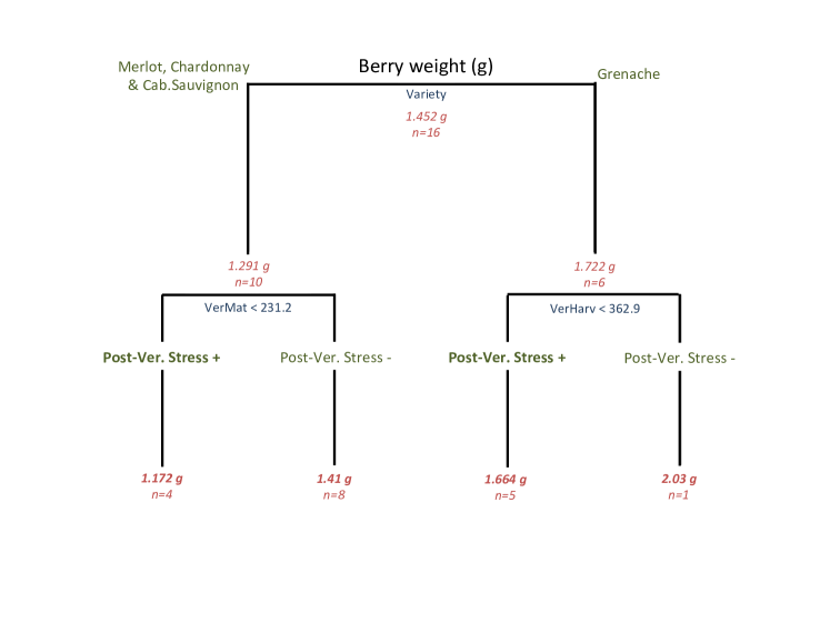
Figure 8: Regression tree explaining Berry Weight ($\mathrm{g}$) using scalars summarizing the three periods, i.e. pre-veraison (NouVer), and post-veraison either until maturity (VerMat) or harvest (VerHarv).

Regarding Sugar Concentration, regression trees show that it is affected by water stress in both pre-veraison NouVer and post-veraison VerHarv periods (Fig.9). The first discriminant variable on Sugar Concentration is the post-veraison water stress (VerHarv, Fig.9). The first split shows that a higher post-veraison water stress leads to a lower Sugar Concentration.

The left branch resulting from the first split shows that the next discriminant variable is again the post-veraison stress VerHarv, so enhancing the effect of the previous split. Lastly, pre-veraison water stress (NouVer) can exacerbate the decrease in Sugar Concentration (as shown in the tree bottom).

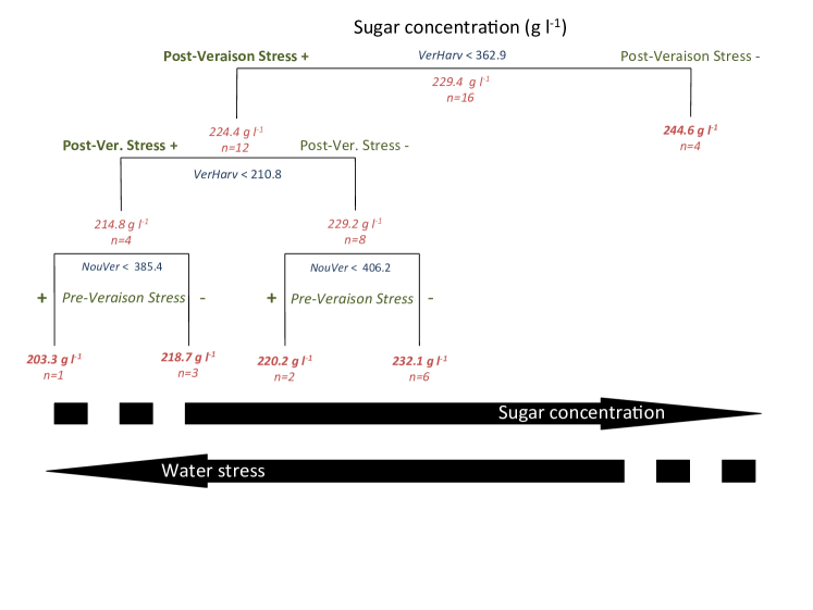
Figure 9: Regression tree explaining Sugar Concentration in berries ($\mathrm{g}\ \reciprocal\mathrm{l}$) using scalars summarizing the three periods, i.e. pre-veraison (NouVer), and post-veraison either until maturity (VerMat) or harvest (VerHarv).

3.2.2 Functional data analysis

Using a continuous indicator of water deficit enables the use of the whole season water stress curve to explain berry composition. This in turn will promote a more precise monitoring of vine water needs according to the targeted fruit composition. Using the FLRTI method James et al. (2009), we analyzed the effects of water stress curve over the season on Berry Weight and Sugar Concentration in berry at harvest.

Regarding Berry Weight, the results showed no significant effect of $\mathit{Ks(t)}$. This was confirmed by applying a specific testing procedure designed for functional linear models, see Hilgert et al. (2013).

Results of the functional data analysis on the effect of $\mathit{Ks(t)}$ on Sugar Concentration are displayed on Fig.10. The tuning parameters are indicated in the legend. Parameters were obtained following a ten-fold cross validation. A sensitivity analysis to small $\sigma$ and $\omega$ variations showed a good robustness of the model, with three main peaks always located in the same time periods across the different varietals. These three main peaks are labeled (1), (2) and (3). Each of them corresponds to a significant effect of $\mathit{Ks}$ on Sugar Concentration which can be positive (peaks (1) and (3)) or negative (peak (2)).

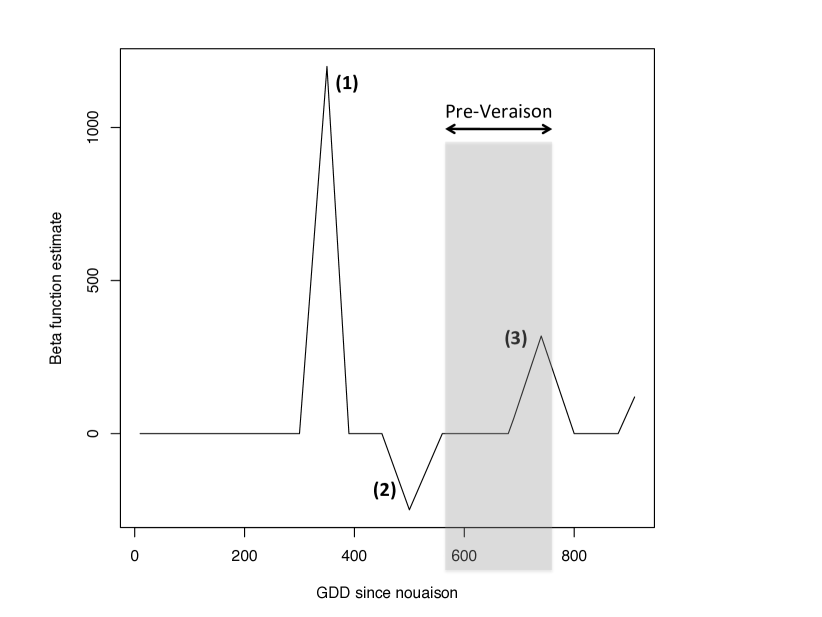
Figure 10: Beta Coefficient evolution over time (see Eq. 7), for explaining Sugar Concentration at harvest. Abscissa are in GDD. The values of $\sigma=0.05$ and $\omega=0.95$ have been found by cross-validation.

Peaks (1) and (3) are positive, which implies a rise in Sugar Concentration. During these periods, the stronger the $\mathit{Ks}$ value, the higher the rise. As $\mathit{Ks}$ varies inversely with water stress, it means that the lower the water stress during these periods, the higher the rise in Sugar Concentration. The effect is twice as strong for the peak (1) than for the peak (3).

Regarding the time period, peak (1) appears to be located before pre-veraison whereas peak (3) occurred during pre-veraison. By contrast, peak (2) has a negative effect on Sugar Concentration. During this period located just before pre-veraison, a low water stress decreases the Sugar Concentration. This can be reformulated as follows: the higher the stress during that period, the lower the decrease in Sugar Concentration.

4 Conclusion

The work presented in this paper used formalized knowledge and mathematical models to design a software sensor from raw data and relate its temporal output to product quality. The proposed approach has been applied to the case of a vine water stress indicator, and its relation to two grape quality variables: Berry Weight and Sugar Concentration.

Results provide a number of meaningful insights.

First of all, the software sensor key point, which is the determination of $K^{*}$, seems reasonably consistent with the literature. From an agronomical point of view, this allows to effectively work at plot scale, and to offer decision support for irrigation, as a function of each plot characteristics.

The use of an ontology allows to separate expert knowledge and numerical models. It makes it much easier to build a generic model, that is both evolutive and adaptable over time as knowledge progresses or climate changes.

Contrary to a data base, an ontology schema adds semantics to the data structure, allowing automatic reasoning, using logical properties, such as reflexivity or transivity.

The ontology presented here has a moderate complexity level: only four kinds of primary concepts, and five types of relations. This is still sufficient to express many mathematical conditions and dependencies, going well beyond the scope of the present case study. There may however be cases where new concepts and relations are necessary, and the ontology can easily be enriched when needed.

Second, the two-fold proposal for data analysis appears to be a good means of exploiting such temporal data as provided by the water stress indicator $\mathit{Ks(t)}$. The results show that the water stress has an effect on grape quality. The analysis confirmed known results on the vine physiological response according to the variety and the irrigation effect. Thus our results are comforting the validity of the $\mathit{Ks}$ indicator, and therefore the level of confidence and reliability in the software sensor design procedure. Functional data analysis highlighted critical periods for vine and berry development, regarding final quality features.

On one hand, the knowledge-based extraction of meaningful summary features over phenological periods of interest allowed to feed these features as input to decision trees. This confirmed the primordial effect played by the variety on Berry Weight determination. On the other hand, functional data analysis made it possible to use the water stress curve ($\mathit{Ks(t)}$), as a whole, to explain Sugar Concentration. This allows more precise monitoring of vine water needs according to a targeted product.

Note that we did not take account of the variety factor in functional data analysis. This would require a covariance analysis model adapted to functional data, which was not possible in this study as the number of data per variety is not sufficient.

These results show the complementarity of both approaches: the first one performs dimensional reduction by summarizing features which requires expert assumptions, the second one handles the continuous temporal data, without any reduction, but it needs more numerous data to be efficient.

Applied perspectives of this work include the study of the relationship between vine water stress and other more complex quality features. In particular new chemical analyses make it possible to follow the aroma development in berries over time, which is assumed to be very sensitive to the grape water status.

Our approach is innovative in more than one aspect. Even if the software sensor had a different design, the same advanced methodology could still be applied to analyze the temporal data. Beyond the present case study, the proposed methodology has a high genericity level, for the applied fields of Agronomy and Environment. It could be used in many cases when raw data have to be transformed by software sensors to be meaningful, or when temporal data have to be analyzed in depth.

References

- Allen et al. (1998) Allen, R. G., Pereira, L. S., Raes, D., Smith, M., 1998. Crop evapotranspiration: Guidelines for computing crop water requirements. Irrigation and Drainage Paper No. 56. FAO, Rome, Italy.
- Ben-David and Sterling (2006) Ben-David, A., Sterling, L., 2006. Generating rules from examples of human multiattribute decision making should be simple. Expert Syst. Appl. 31 (2), 390–396.
- Breiman et al. (1984) Breiman, L., Friedman, J., Olshen, R., Stone, C., 1984. Classification and regression trees. Wadsworth, Belmont, CA 1.
-
Cifre et al. (2005)
Cifre, J., Bota, J., Escalona, J., Medrano, H., Flexas, J., Apr. 2005.
Physiological tools for irrigation scheduling in grapevine (Vitis vinifera
L.)An open gate to improve water-use efficiency? Agriculture, Ecosystems &
Environment 106 (2-3), 159–170.
URL http://linkinghub.elsevier.com/retrieve/pii/S0167880904%002956 - Destercke et al. (2013) Destercke, S., Buche, P., Charnomordic, B., jan. 2013. Evaluating data reliability: An evidential answer with application to a web-enabled data warehouse. Knowledge and Data Engineering, IEEE Transactions on 25 (1), 92 –105.
- Escalona et al. (2002) Escalona, J., Flexas, J., Medrano, H., 2002. Drought effects on water flow, photosynthesis and growth of potted grapevines. Vitis 41, 57–62.
-
Ferreira et al. (2012)
Ferreira, M. I., Silvestre, J., Conceição, N., Malheiro, A. C., Jun.
2012. Crop and stress coefficients in rainfed and deficit irrigation
vineyards using sap flow techniques. Irrigation Science 30 (5), 433–447.
URL http://www.springerlink.com/index/10.1007/s00271-012-03%52-2 - Ginestar et al. (1998) Ginestar, C., Eastham, J., Gray, S., Iland, P., 1998. Use of sap flow sensors to shedule vineyard irrigation. 1. effects of post-veraison water deficit on water relation, vine growth, and yield of shiraz grapevines. Am. J. Enol. Vitic. 49, 413–420.
- Guarino et al. (2009) Guarino, N., Oberle, D., Staab, S., 2009. Handbook on Ontologies, 2nd Edition. Springer, Ch. What is an Ontology?
- Hilgert et al. (2013) Hilgert, N., Mas, A., Verzelen, N., 2013. Minimax adaptive tests for the functional linear model. The Annals of Statistics 41 (2), 838–869.
- James et al. (2009) James, G. M., Wang, J., Zhu, J., 2009. Functional linear regression that’s interpretable. The Annals of Statistics 37, 2083–2108.
-
Jones (2004)
Jones, H. G., Nov. 2004. Irrigation scheduling: advantages and pitfalls of
plant-based methods. Journal of experimental botany 55 (407), 2427–36.
URL http://www.ncbi.nlm.nih.gov/pubmed/15286143 - Miller (1956) Miller, G. A., 1956. The magical number seven, plus or minus two: Some limits on our capacity for processing information. Psychological Review 63, 81–97.
- Musen (1992) Musen, M., 1992. Dimensions of knowledge sharing and reuse. Computers and Biomedical Research 25 (5), 435–467.
- Olivo et al. (2009) Olivo, N., Girona, J., Marsal, J., 2009. Seasonal sensitivity of stem water potential to vapour pressure deficit in grapevine. Irrigation Science 27, 175–182.
- Parker et al. (2011) Parker, A., De Cortázar-Atauri, I., Van Leeuwen, C., Chuine, I., 2011. General phenological model to characterize the timing of flowering and veraison of vitis vinifera l. Australian Journal of Grape and Wine Research 17, 206–216.
-
Picón-Toro et al. (2012)
Picón-Toro, J., González-Dugo, V., Uriarte, D., Mancha, L. a., Testi,
L., Jun. 2012. Effects of canopy size and water stress over the crop
coefficient of a Tempranillo vineyard in south-western Spain. Irrigation
Science 30 (5), 419–432.
URL http://www.springerlink.com/index/10.1007/s00271-012-03%51-3 - Quinlan (1986) Quinlan, J., 1986. Induction of decision trees. Machine learning 1 (1), 81–106.
- Quinlan (1993) Quinlan, J., 1993. C4. 5: programs for machine learning. Morgan Kaufmann.
-
R Development Core Team (2009)
R Development Core Team, 2009. R: A Language and Environment for Statistical
Computing. R Foundation for Statistical Computing, Vienna, Austria, ISBN
3-900051-07-0.
URL http://www.R-project.org - Ramsay and Silverman (2005) Ramsay, J. O., Silverman, B. W., 2005. Functional data analysis, 2nd Edition. Springer Series in Statistics. Springer, New York.
- Rijgersberg et al. (2013) Rijgersberg, H., van Assem, M., Top, J. L., 2013. Ontology of units of measure and related concepts. Semantic Web 4 (1), 3–13.
- Rodrigues et al. (2012) Rodrigues, P., Pedroso, V., Gouveia, J. P., Martins, S., Lopes, C., Alves, I., 2012. Influence of soil water content and atmospheric conditions on leaf water potential in cv. touriga nacional deep-rooted vineyards. Irrigation Science 30, 407–417.
- Santesteban et al. (2009) Santesteban, L. G., Miranda, C., Royo, J. B., 2009. Suitability of pre-dawn and stem water potential as indicators of vineyard water status in cv . Tempranillo. Society.
- Thomopoulos et al. (2013) Thomopoulos, R., Destercke, S., Charnomordic, B., Iyan, J., Abécassis, J., Feb. 2013. An iterative approach to build relevant ontology-aware data-driven models. Information Sciences 221, 452–472.
-
Ullah and Finch (2013)
Ullah, S., Finch, C. F., 2013. Applications of functional data analysis: A
systematic review. BMC Medical Research Methodology 13 (1), 43.
URL http://www.biomedcentral.com/1471-2288/13/43 - Villanueva-Rosales and Dumontier (2008) Villanueva-Rosales, N., Dumontier, M., 2008. Modeling life science knowledge with owl 1.1. In: Proceedings of OWL’08.
- Williams and Baeza (2007) Williams, L., Baeza, P., 2007. Relationships among ambient temperature and vapor pressure deficit and leaf and stem water potentials of fully irrigated , field-grown grapevines. Am. J. Enol. Vitic. 58, 2.
-
Williams and Ayars (2005)
Williams, L. E., Ayars, J. E., Oct. 2005. Grapevine water use and the crop
coefficient are linear functions of the shaded area measured beneath the
canopy. Agricultural and Forest Meteorology 132 (3-4), 201–211.
URL http://dx.doi.org/10.1016/j.agrformet.2005.07.010 -
Zhang et al. (2011)
Zhang, Y., Kang, S., Ward, E. J., Ding, R., Zhang, X., Zheng, R., 2011.
Evapotranspiration components determined by sap flow and microlysimetry
techniques of a vineyard in northwest China: Dynamics and influential
factors. Agricultural Water Management.
URL http://dx.doi.org/10.1016/j.agwat.2011.03.006