Singularities, boundary conditions and gauge link in the light cone gauge

Abstract

In this work, we first review the issues on the singularities and the boundary conditions in light cone gauge and how to regularize them properly. Then we will further review how these singularities and the boundary conditions can result in the gauge link at the infinity in the light cone direction in the Drell-Yan process. Except for reviewing, we also have verified that the gauge link at the light cone infinity has no dependence on the path not only for the Abelian field but also for non-Abelian gauge field.

I introduction

The light cone gauge was widely used as an approach to remove the redundant freedom in quantum gauge theories. The Yang-Mills theories were studied on the quantization in light cone gauge by several authors Bassetto:1984dq ; Leibbrandt:1983pj . In perturbative QCD, the collinear factorization theorems of hard processes can be proved more conveniently and simply in light cone gauge than in other gauges Amati:1978by ; Ellis:1978ty ; Efremov:1978cu ; Libby:1978qf ; Libby:1978bx . Actually only in light cone gauge, the parton distribution functions defined in QCD hold the probability interpretation in the naive parton modelFey71 . However in light cone gauge, when we calculate the Feynman diagrams with the gauge propagator in the perturbative theory, we have to deal with the light cone singularity $1/q^{+}$,

$$D_{\mu\nu}(q)=\frac{1}{q^{2}+i\epsilon}\left(g_{\mu\nu}-\frac{n_{\mu}q_{\nu}+n_{\nu}q_{\mu}}{q^{+}}\right).$$ (1)

There have been a variety of prescriptions suggested to handle such singularities Bassetto:1983bz ; Lepage:1980fj ; Leibbrandt:1987qv ; Slavnov:1987yh ; Kovchegov:1997pc from a practical point of view. Afterwards, it was clarified Bassetto:1981gp that the gauge potential cannot be arbitrarily set to vanish at the infinity in the light cone gauge, the spurious singularities are physically related to the boundary conditions that one can impose on the potentials at the infinity. Different pole structures for regularization mean different boundary conditions. It should be emphasized that the above conclusion does not restrict to the light cone gauge, it holds for any axial gauges.

The non-trivial boundary conditions at the infinity in the light cone gauge also clarifies another puzzle in the transverse momentum dependent structure functions of nucleons. In the covariant gauge, in which the gauge potential vanishes at the space-time infinity, the transverse-momentum parton distribution can be given by operator matrix elements Collins:1981uw ; Collins:1989bt ; Collins:2003fm

$$q(x,\vec{k}_{\perp}) = \frac{1}{2}\int\frac{dy^{-}}{2\pi}\frac{d^{2}{\bf{y}}_{\perp}}{(2\pi)^{2}}{\rm e}^{-ixp^{+}y^{-}+i{\bf{k}}_{\perp}\cdot{\bf{y}}_{\perp}}$$ (2)

$$\times\langle P|\bar{\psi}(y^{-},{\bf{y}}_{\perp})n\!\!\!/\mathcal{L}^{\dagger}[\infty,{\bf{y}}_{\perp};y^{-},{\bf{y}}_{\perp}]$$

$$\times\mathcal{L}[\infty,{\bf{0}}_{\perp};0,{\bf{0}}_{\perp}]\psi(0,{\bf{0}}_{\perp})|P\rangle\,,$$

where

$$\mathcal{L}[\infty,{\bf{y}}_{\perp};y^{-},{\bf{y}}_{\perp}]\equiv P\exp\left(-ig\int_{y^{-}}^{\infty}d\xi^{-}A^{+}(\xi^{-},{\bf{y}}_{\perp})\right)\,,$$ (3)

is the gauge link or wilson line to ensure the gauge invariance of the matrix elements. Such gauge link is produced from final state interactions between the struck quark and the target spectators. It has been verified in Ref.Collins:1992kk that the presence of the gauge link is essential for the non-vanishing Sivers function, which is the main mechanism of single spin asymmetry at low transverse momentum in high energy collisions. However if we naively choose the light cone gauge $A^{+}=0$ in the above definition, it seems as if the gauge link in Eq. (3) would disappear, which would result in the final interaction or Siver’s function vanishing. It seems as if different gauges lead to contradictory results. Since physics should not depend on the gauge we choose, there must be something we missed in the above. Such contradiction was solved by Ji and Yuan in Ji:2002aa where they found that the final state interaction effects can be recovered properly in the light cone gauge by introducing a transverse gauge link at the light cone infinity. Then in Belitsky:2002sm , Belitsky, Ji, and Yuan demonstrated how the transverse gauge link can be produced from the transverse components of the gauge potential at the light cone infinity at the leading twist level. Further in Gao:2010sd , we derived such transverse gauge link within a more regular and general method. It was found that the gauge link at light cone infinity naturally arises from the contribution of the pinched poles: one is from the quark propagator and the other is hidden in the gauge vector field in the light cone gauge. It is just the pinched poles that pick out the contribution of the gauge potential at the light cone infinity. Actually in Gao:2010sd , a more general gauge link over the hypersurface at the light cone infinity was derived, which is beyond the transverse direction. Besides, there are also other relevant works on the transverse gauge link in the literature Boer:2003cm ; Idilbi:2008vm ; Cherednikov:2011ku .

In this paper, we will devote ourselves to reviewing the above works and putting them together with the emphasis on mathematical rigor. However, through the reviewing, we will try to discuss them in a different way or point of view, which can be also regarded as the complementary to the previous work. Except for reviewing, we also have verified that the gauge link at the light cone infinity has no dependence on the path not only for the Abelian field but also for non-Abelian gauge field, which has not been discussed in the previous works.

We will organize the paper as follows: in Sec. II, we present some definitions and notations which will be used in our paper. In Sec. III, we discuss how the singularity can arise in the light cone gauge, how different singularities correspond to different boundary conditions and how we regularize them properly. In Sec. IV, we derive the transverse gauge link or more general gauge link in light cone gauge in Drell-Yan process. In Sec. V, we verify that the gauge link at the light cone infinity has no dependence on the path for non-Abelian gauge field. In Sec. VI, we give a brief summary.

II definitions and notations

In our work, we will choose the light cone coordinate system by introducing two lightlike vectors $n^{\mu}$ and $\bar{n}^{\mu}$ and two transverse spacelike vectors $n_{\perp 1}^{\mu}$ and ${n}_{\perp 2}^{\mu}$

$$n^{\mu} = \frac{1}{\sqrt{2}}\left(1,0,0,1\right)\equiv[0,1,{\bf{0}}_{\perp}],\$$ (4)

$$\bar{n}^{\mu} = \frac{1}{\sqrt{2}}\left(1,0,0,-1\right)\equiv[1,0,{\bf{0}}_{\perp}]$$ (5)

$$n_{\perp 1}^{\mu} = (0,0,1,0)\equiv[0,0,1,0],$$ (6)

$$n_{\perp 2}^{\mu} = (0,0,0,1)\equiv[0,0,0,1]$$ (7)

where we have used square brackets ‘[ ]’ to denote the components in the light-cone coordinate, compared with the usual Cartesian coordinate denoted by the parentheses ‘( )’. In such coordinate system, we can write any vector $k^{\mu}$ as $[k^{+},k^{-},{\bf{k}}_{\perp}]$ or $[k^{+},k^{-},{k}_{\perp 1},{k}_{\perp 2}]$, where $k^{+}=k\cdot n,\ k^{-}=k\cdot\bar{n},\ k_{\perp 1}=n_{\perp 1}\cdot k,\ k_{\perp 2}=n_{\perp 2}\cdot k$.

Since we will consider the non-Abelian gauge field all through our paper, we will use the usual compact notations for the non-Abelian field potential and strength, respectively,

$${A}_{\mu}\equiv{A}^{a}_{\mu}t^{a},\ \ F_{\mu\nu}\equiv F^{a}_{\mu\nu}t^{a},$$ (8)

where $t^{a}$ is the fundamental representation of the generators of the gauge symmetry group.

For the sake of conciseness, we would like to introduce some further notations. We will decompose any momentum vector $k^{\mu}$ and the gauge potential vector $A^{\mu}$, as the following

$$k^{\mu} = {\tilde{k}}^{\mu}+xp^{\mu},\ \ A^{\mu}={\tilde{A}}^{\mu}+A^{+}\bar{n}^{\mu}$$ (9)

where ${\tilde{k}}^{\mu}=[0,k^{-},{\bf{k}}_{\perp}]$, $x=k^{+}/p^{+}$, and $\tilde{A}^{\mu}=[0,A^{-},{\bf{A}}_{\perp}]$. Meanwhile, for any coordinate vector $y^{\mu}$ , we will make the following decomposition,

$$y^{\mu} = {\dot{y}}^{\mu}+y^{-}n^{\mu}$$ (10)

where $\dot{y}^{\mu}=[y^{+},0,{\bf{y}}_{\perp}]$. With these notations, it is very easy to show $k\cdot y=\tilde{k}\cdot\dot{y}+xp^{+}y^{-}$. In the light cone gauge $A^{+}=0$, the gauge vector $A^{\mu}={\tilde{A}}^{\mu}$. When no confusion could arise, we will write $y^{\mu}$ as $[y^{-},\dot{y}]$ for simplicity.

III singularities and boundary conditions in the light cone gauge

In this section, we will review how the singularities appear in the light cone gauge, how they are related to the boundary conditions of the gauge potential at the light cone infinity and how we can regularize them in a proper way consistent with the boundary conditions. Although this section is mainly based on the literature Bassetto:1981gp and Belitsky:2002sm , there are also a few differences from them. For example, we will discuss the non-Abelian gauge field from the beginning to the end, while in the original works, only the Abelian gauge field was emphasized. Besides we will make the maximal gauge fixing from the point of view of linear differential equation.

With the light cone gauge condition $n_{\mu}A^{\mu}=0$, let us consider the non-Abelian counterpart of Maxwell equations,

$$D_{\mu}F^{\mu\nu}=-j^{\nu}$$ (11)

where $F_{\mu\nu}=\partial_{\mu}A_{\nu}-\partial_{\nu}A_{\mu}-ig\left[A_{\mu},A_{\nu}\right],\ \ j^{\nu}=\bar{\psi}t^{a}\gamma^{\nu}\psi t^{a}$. We can rewrite the above equations in another form

$$\partial_{\mu}\partial^{\mu}A^{\nu}-\partial^{\nu}\partial_{\mu}A^{\mu}=-J^{\nu}$$ (12)

where we have defined $J^{\nu}\equiv j^{\nu}+ig[A_{\mu},F^{\mu\nu}]+ig\partial_{\mu}[A^{\mu},A^{\nu}]$. Contracting both sides of Eq.(12) with $n_{\nu}$ and taking the light cone gauge condition into account yields

$$n_{\nu}\partial^{\nu}\partial_{\mu}\tilde{A}^{\mu}=n_{\nu}J^{\nu}.$$ (13)

Integrating the above equation gives rise to

$$\tilde{\partial}_{\mu}\tilde{A}^{\mu}(+\infty,\tilde{x})-\tilde{\partial}_{\mu}\tilde{A}^{\mu}(-\infty,\tilde{x})=\int_{-\infty}^{+\infty}dx^{-}n_{\nu}J^{\nu}$$ (14)

Since $\int_{-\infty}^{+\infty}dx^{-}n_{\nu}J^{\nu}=0$, in general, need not be true, we can not arbitrarily choose both $A^{\mu}(+\infty,\tilde{x})=0$ and $A^{\mu}(-\infty,\tilde{x})=0$ at the same time. One of these boundary conditions can be arbitrarily chosen while the other one must be subjected to satisfy the constraint (14). This is just why we can not choose the boundary conditions arbitrarily in light cone gauge. In fact, this conclusion holds for any axial gauges. From the Fourier transforms of Eq.(12),

$$k^{2}\mathcal{A}^{\nu}-k^{\nu}(k\cdot\mathcal{A})=-\mathcal{J}$$ (15)

and together with the light cone gauge condition, it is easy to obtain the formal solutions

$$\tilde{A}^{\mu}=\int d^{4}k\frac{e^{ik\cdot x}}{k^{2}}\left(-\mathcal{\tilde{J}}^{\mu}+\frac{\tilde{k}^{\mu}}{k^{+}}{\mathcal{J}}^{+}\right)$$ (16)

where $\mathcal{A}^{\mu}$ and $\mathcal{J}^{\mu}$ are the Fourier transforms of $A^{\mu}$ and $J^{\mu}$,respectively. It is obvious that there is an extra singularity at $k^{+}=0$ in the solution (16). If we assume that the currents are regular at $k=0$, it is easy to verify that the different pole prescriptions correspond to different boundary conditions. In our paper, we will consider three different boundary conditions,

Advanced $$: \ \tilde{A}(+\infty,\dot{y})=0$$

Retarded $$: \ \tilde{A}(-\infty,\dot{y})=0$$

Antisymmetric $$: \ \tilde{A}(-\infty,\dot{y})+\tilde{A}(\infty,\dot{y})=0$$ (17)

which correspond to three different pole structures, respectively,

$$\ \frac{1}{k^{+}-i\epsilon},\ \ \ \ \ \frac{1}{k^{+}+i\epsilon},\ \ \ \ \frac{1}{2}\left(\frac{1}{k^{+}+i\epsilon}+\frac{1}{k^{+}-i\epsilon}\right).$$ (18)

where the last prescription is just the conventional principal value regularization. In the next section, we will deal with the Fourier transform of the gauge potential,

$$\tilde{\cal{A}}_{\mu}(k^{+},\dot{y})\equiv\int_{-\infty}^{\infty}dy^{-}\textrm{e}^{ik^{+}y^{-}}\tilde{A}_{\mu}(y^{-},\dot{y})$$ (19)

In order to pick out the contribution of the gauge potential at the infinity, we need a mathematical trick by manipulating this integration by parts,

$$\int_{-\infty}^{\infty}dy^{-}\textrm{e}^{ik^{+}y^{-}}\tilde{A}_{\mu}(y^{-},\dot{y})$$ (20)

$$= \frac{i}{k^{+}}\int_{-\infty}^{\infty}dy^{-}\textrm{e}^{ik^{+}y^{-}}\partial^{+}\tilde{A}_{\mu}(y^{-},\dot{y})$$

where $\partial^{+}=\partial_{-}={\partial}/{\partial y^{-}}$. We will see that once we choose the prescriptions (18) according to the boundary conditions (III), we will obtain the gauge link at the light cone infinity.

We have seen that we cannot choose the boundary conditions arbitrarily, now we will discuss how to fix the gauge freedom as maximally as possible. These have been also discussed in the appendix in Ref.Belitsky:2002sm , we will take them into account from the point of view of differential equations. Under a general gauge transformation, the gauge potential transforms as,

$$A_{\mu}\rightarrow S^{-1}A_{\mu}S+\frac{i}{g}S^{-1}\partial_{\mu}S$$ (21)

In order to eliminate the light cone component $n\cdot A=0$, we obtain the gauge transformation by solving the equation,

$$n^{\mu}\partial_{\mu}S=ign^{\mu}A_{\mu}S$$ (22)

This equation is an ordinary linear differential equation, whose solution is well known,

$$S = {P}\left\{\textrm{exp}\left[ig\int_{x_{0}^{+}}^{x^{+}}n^{\mu}A_{\mu}\left(\xi,x^{-},x_{\perp 1},x_{\perp 2}\right)d\xi\right]\right\}$$ (23)

$$\times\tilde{S}(x^{-},x_{\perp 1},x_{\perp 2})$$

where $S(x^{-},x_{\perp 1},x_{\perp 2})$ is an arbitrary unitary matrix which does not depend on $x^{+}$. This freedom allows us to set one of the residual three components of $A_{\mu}$ zero on the three dimensional hyperplane at $x^{+}=x_{0}^{+}$. Without loss of generality, we can set $A^{-}(x_{0}^{+},x^{-},x_{\perp})=0$ by solving the following equation

$$\bar{n}^{\mu}\partial_{\mu}\tilde{S}=ig\bar{n}^{\mu}A_{\mu}\tilde{S}.$$ (24)

The solution is given by

$$\tilde{S} = {P}\left\{\textrm{exp}\left[ig\int_{x_{0}^{-}}^{x^{-}}d\xi\bar{n}^{\mu}A_{\mu}\left(x_{0}^{+},\xi,x_{\perp 1},x_{\perp 2}\right)\right]\right\}$$ (25)

$$\times S_{\perp}(x_{\perp 1},x_{\perp 2}).$$

There is still an arbitrary unitary matrix which depends only on $x_{\perp}$. We can use this freedom to further set one of the residual transverse components of the gauge potential zero, e,g, $A_{\perp 1}$=0, at the two dimensional hyperplane ($x^{+}=x_{0}^{+}$, $x^{-}=x_{0}^{-}$) by solving

$$n_{\perp 1}^{\mu}\partial_{\mu}S_{\perp}=ign_{\perp 1}^{\mu}A_{\mu}S_{\perp}(x_{\perp 1},x_{\perp 2})$$ (26)

The solution is given by

$$S_{\perp} = {P}\left\{\textrm{exp}\left[ig\int_{x_{0\perp 1}}^{x_{\perp 1}}d\xi n_{\perp 1}^{\mu}A_{\mu}\left(x_{0}^{+},x_{0}^{-},\xi,x_{\perp 2}\right)\right]\right\}$$ (27)

$$\times S_{1\perp}(x_{\perp 2}).$$

We can continue to set the only left transverse components $A_{\perp 2}=0$ at the straight line [$x^{+}=x_{0}^{+}$, $x^{-}=x_{0}^{-}$, $x_{\perp 1}=x_{0\perp 1}$] by solving

$$n_{\perp 2}^{\mu}\partial_{\mu}S_{1\perp}=ign_{\perp 2}^{\mu}A_{\mu}S_{1\perp}(x_{\perp 2})$$ (28)

The solution is given by

$$S_{1\perp} = {P}\left\{\textrm{exp}\left[ig\int_{x_{0\perp 1}}^{x_{\perp 1}}d\xi n_{\perp 2}^{\mu}A_{\mu}\left(x_{0}^{+},x_{0}^{-},x_{0\perp 2},\xi\right)\right]\right\}$$ (29)

$$\times S_{2\perp}$$

With only a trivial global gauge transformation left, we have maximally fixed our gauge freedom. Although we cannot choose the boundary conditions of the gauge potential arbitrarily in the light cone gauge, the constraint that the field strengths should vanish at the infinity requires that the gauge potential must be a pure gauge,

$${A}_{\mu}=\frac{1}{ig}\omega^{-1}{\partial}_{\mu}\omega$$ (30)

where $\omega=\textrm{exp}(i\phi)$ with $\phi\equiv\phi^{a}t^{a}$. We can expand the above pure gauge as

$$A_{\mu} = \frac{1}{ig}\omega^{-1}{\partial}_{\mu}\omega$$ (31)

$$= \partial_{\mu}\phi+\frac{i}{2!}\left[\partial_{\mu}\phi,\phi\right]+\frac{i^{2}}{3!}\left[\left[\partial_{\mu}\phi,\phi\right],\phi\right]+\cdot\cdot\cdot\ \ \$$

IV Gauge link in the light cone gauge in Drell-Yan process

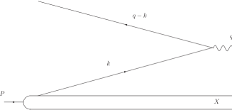
Figure 1: The tree diagram in Drell-Yan process

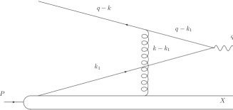
Figure 2: The one-gluon exchange diagram in Drell-Yan process

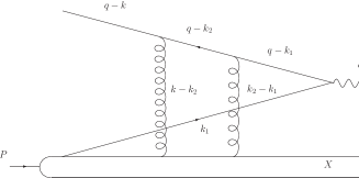
Figure 3: The two-gluon exchange diagram in Drell-Yan process

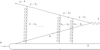
Figure 4: The $n$-gluon exchange diagram in Drell-Yan process

In this section, we will review how the singularities and boundary conditions in the light cone gauge can result in the gauge link at the light cone infinity. Since the detailed derivation of transverse gauge link had been made for semi-inclusive deeply inelastic scattering Belitsky:2002sm ; Gao:2010sd , we will discuss the Drell-Yan process in details in order to avoid total repeating. For simplicity, we will set the target to be a nucleon and the projectile be just an antiquark.

The tree scattering amplitude of Drell-Yan process corresponding to Fig. 1 reads

$$M_{0}^{\mu}=\bar{u}(q-k)\gamma^{\mu}\langle X|\psi(0)|P\rangle\,,$$ (32)

where $k$ denotes the momentum of initial quark from the proton $P$ with the momentum $p$, and $q-k$ and $q$ are the momenta of the anti-quark and virtual photon, respectively.

The one-gluon amplitude in the light cone gauge corresponding to Fig. 2 reads,

$$M_{1}^{\mu} = \int\frac{d^{4}k_{1}}{(2\pi)^{4}}d^{4}y_{1}\ e^{i(k-k_{1})\cdot y_{1}}\bar{u}(q-k)\gamma^{\rho_{1}}\frac{{q\!\!\!/-k\!\!\!/}_{1}\!\!}{(q-k_{1})^{2}+i\epsilon}$$ (33)

$$\times\langle X|\tilde{A}_{\rho_{1}}(y_{1})\gamma^{\mu}\psi(0)|P\rangle\,.$$

In order to obtain the leading twist contribution, we only need the pole contribution in the quark propagator,

$$\hat{M}_{1}^{\mu} = \int\frac{d^{3}\tilde{k}_{1}}{(2\pi)^{4}}d^{3}\dot{y}_{1}\frac{p^{+}dx_{1}}{2\pi}dy_{1}^{-}\ e^{i(\tilde{k}-\tilde{k}_{1})\cdot\dot{y}_{1}+i({x}-{x}_{1})p^{+}y^{-}}$$ (34)

$$\times\bar{u}(q-\hat{k})\gamma^{\rho_{1}}\frac{q\!\!\!/\!\!-{\hat{k}\!\!\!/}_{1}}{2p\cdot(\hat{k}_{1}-q)}\frac{1}{(x_{1}-\hat{x}_{1}-i\epsilon)}$$

$$\times\langle X|\tilde{A}_{\rho_{1}}(y_{1})\gamma^{\mu}\psi(0)|P\rangle$$

where $\hat{M}_{1}^{\mu}$ with an extra $\hat{\ }$ denotes that only the pole contribution is kept and $\hat{k}_{1}\equiv[\hat{x}_{1}p^{+},k_{1}^{-},k_{1\perp}]$ with $\ \hat{x}_{1}=\hat{k}^{+}/p^{+}=x_{B}+k_{\perp}^{2}/2p\cdot(k_{1}-q)\$, which is determined by the on-shell condition $\ (q-\hat{k}_{1})^{2}=0\$. In Eq.(34), we have separated the integral over $x_{1}$ and $y^{-}_{1}$ from the others in order to finish integrating them out first. Now we need to choose a specific boundary condition for the gauge potential $\tilde{A}_{\rho}$ at the infinity. Let us start with the advanced boundary condition $\tilde{A}(+\infty,\dot{y})=0$. Using Eq. (20) for the advanced boundary condition, we have

$$\hat{M}_{1}^{\mu} = \int\frac{d^{3}\tilde{k}_{1}}{(2\pi)^{4}}\int d^{3}\dot{y}_{1}\ \int\frac{dx_{1}}{2\pi}\int dy_{1}^{-}$$ (35)

$$\times e^{i(\tilde{k}-\tilde{k}_{1})\cdot\dot{y}_{1}}e^{i({x}-{x}_{1})p^{+}y^{-}}\bar{u}(q-k)\gamma^{\rho_{1}}$$

$$\times\frac{{q\!\!\!/-\hat{k}\!\!\!/}_{1}\!\!}{2p\cdot(\hat{k}_{1}-q)}\frac{1}{(x_{1}-\hat{x}_{1}-i\epsilon)}\frac{i}{({x}-{x}_{1}-i\epsilon)}$$

$$\times\langle X|\partial^{+}\tilde{A}_{\rho_{1}}(y_{1})\gamma^{\mu}\psi(0)|P\rangle\hskip 14.22636pt$$

Finish integrating over $x_{1}$ and $y_{1}^{-}$:

$$\int\frac{dx_{1}}{2\pi}dy_{1}^{-}e^{i({x}-{x}_{1})p^{+}y^{-}}\frac{1}{(x_{1}-\hat{x}_{1}-i\epsilon)}$$ (36)

$$\times\frac{i}{(x-{x}_{1}-i\epsilon)}\partial^{+}\tilde{A}_{\rho_{1}}(y_{1})$$

$$= -\int dy_{1}^{-}\left(\theta(-y^{-})e^{i({x}-\hat{x}_{1})p^{+}y^{-}}+\theta(y^{-})\right)$$

$$\times\frac{1}{{x}-\hat{x}_{1}}\partial^{+}\tilde{A}_{\rho_{1}}(y_{1})$$

$$= \frac{1}{{x}-\hat{x}_{1}}\tilde{A}_{\rho_{1}}(-\infty,\dot{y}_{1})+\textrm{higher twist}\,.$$

where only the leading term in the Tailor expansion of the phase factor $e^{i({x}-\hat{x}_{1})p^{+}y^{-}}$ is kept, because the other terms are proportional to $({x}-\hat{x}_{1})^{n}=\left[k_{\perp}^{2}/2p\cdot(k+q)-k_{1\perp}^{2}/2p\cdot(k_{1}+q)\right]^{n}$ $(n\geq 1)$, which will contribute at higher twist level.

However if we choose the retarded boundary conditions, we can have

$$\hat{M}_{1}^{\mu} = \int\frac{d^{3}\tilde{k}_{1}}{(2\pi)^{4}}\int d^{3}\dot{y}_{1}\ \int\frac{dx_{1}}{2\pi}\int dy_{1}^{-}$$ (37)

$$\times e^{i(\tilde{k}-\tilde{k}_{1})\cdot\dot{y}_{1}}e^{i({x}-{x}_{1})p^{+}y^{-}}\bar{u}(q-k)\gamma^{\rho_{1}}$$

$$\frac{{q\!\!\!/-\hat{k}\!\!\!/}_{1}\!\!}{2p\cdot(\hat{k}_{1}-q)}\frac{1}{(x_{1}-\hat{x}_{1}-i\epsilon)}\frac{i}{({x}-{x}_{1}+i\epsilon)}$$

$$\times\langle X|\partial^{+}\tilde{A}_{\rho_{1}}(y_{1})\gamma^{\mu}\psi(0)|P\rangle.\hskip 14.22636pt$$

Integrating out $x_{1}$ and $y_{1}^{-}$ first yields

$$\int\frac{dx_{1}}{2\pi}\int dy_{1}^{-}e^{i({x}-{x}_{1})p^{+}y^{-}}\frac{1}{(x_{1}-\hat{x}_{1}-i\epsilon)}$$ (38)

$$\times\frac{i}{(x-{x}_{1}+i\epsilon)}\partial^{+}\tilde{A}_{\rho_{1}}(y_{1})$$

$$= -\int dy_{1}^{-}\left(\theta(-y^{-})e^{i({x}-\hat{x}_{1})p^{+}y^{-}}-\theta(-y^{-})\right)$$

$$\times\frac{1}{{x}-\hat{x}_{1}}\partial^{+}\tilde{A}_{\rho_{1}}(y_{1})$$

$$= \textrm{higher twist}\,.$$

We can see the retarded boundary condition does not result in leading twist contribution in the Drell-Yan process. If we choose the antisymmetric boundary condition, which corresponds to the principal value regularization, we obtain

$$\int\frac{dx_{1}}{2\pi}\int dy_{1}^{-}e^{i({x}-{x}_{1})p^{+}y^{-}}\frac{1}{(x_{1}-\hat{x}_{1}+i\epsilon)}$$ (39)

$$\times\textrm{PV}\frac{i}{(x-{x}_{1})}\partial^{+}\tilde{A}_{\rho_{1}}(y_{1})$$

$$= \int dy_{1}^{-}\frac{1}{2}\left(2\theta(y^{-})e^{i({x}-\hat{x}_{1})p^{+}y^{-}}-\theta(y^{-})+\theta(-y^{-})\right)$$

$$\times\frac{1}{{x}-\hat{x}_{1}}\partial^{+}\tilde{A}_{\rho_{1}}(y_{1})$$

$$= \frac{1}{{x}-\hat{x}_{1}}\tilde{A}_{\rho_{1}}(+\infty,\dot{y}_{1})+\textrm{higher twist}\,,$$

where PV denotes principal value. In the above derivation, we notice that the presence of the pinched poles are necessary to pick up the gauge potential at the light cone infinity. Actually these pinched poles have selected the so-called Glauber modes of the gauge fieldIdilbi:2008vm . Although there is no leading twist contribution in the retarded boundary condition, it was shown in Belitsky:2002sm , that all the final state interactions have been encoded into the initial state light cone wave functions. In principal value regularization, the final state scattering effects appear only through the gauge link , while in advanced regularization, it appear through both the gauge link and initial light cone wave functions. In the following, we will only concentrate on the advanced boundary condition. Only keep leading twist contribution and inserting Eq. (36) into Eq. (35), we have

$$\hat{M}_{1} = \int\frac{d^{3}\tilde{k}_{1}}{(2\pi)^{4}}d^{3}\dot{y}_{1}\ e^{i(\tilde{k}-\tilde{k}_{1})\cdot\dot{y}_{1}}\bar{u}(q-{k})\gamma^{\rho_{1}}\frac{q\!\!\!/-{\hat{k}\!\!\!/}_{1}}{2p\cdot(\hat{k}_{1}-q)}$$ (40)

$$\times\frac{1}{{x}-\hat{x}_{1}}\langle X|\tilde{A}_{\rho_{1}}(-\infty,\dot{y}_{1})\psi(0)|P\rangle\,.\hskip 8.5359pt$$

Using Eq. (31), only keeping the first Abelian term and performing the integration by parts over $\dot{y}_{1}$, we obtain

$$\hat{M}_{1} = \int\frac{d^{3}\tilde{k}_{1}}{(2\pi)^{4}}d^{3}\dot{y}_{1}\ e^{i(\tilde{k}-\tilde{k}_{1})\cdot\dot{y}_{1}}\bar{u}(q-{k})(\tilde{k}\!\!\!/-\tilde{k}\!\!\!/_{1})$$ (41)

$$\times\frac{q\!\!\!/-{\hat{k}\!\!\!/}_{1}}{2p\cdot(\hat{k}_{1}-q)}\frac{-i}{{x}-\hat{x}_{1}}\langle X|\phi(-\infty,\dot{y}_{1})\psi(0)|P\rangle.\hskip 19.91684pt$$

We can calculate these Dirac algebras and finally obtain,

$$\hat{M}_{1} = \bar{u}(q-k)\langle X|i\phi(-\infty,{0})\psi(0)|P\rangle\,.$$ (42)

where we have dropped all the higher twist contributions. Now let us further consider the two-gluon exchange scattering amplitude plotted in Fig. 3,

$$M_{2}^{\mu} = \int\frac{d^{4}k_{2}}{(2\pi)^{4}}\frac{d^{4}k_{1}}{(2\pi)^{4}}d^{4}y_{2}d^{4}y_{1}\ e^{i(k-k_{2})\cdot y_{2}+i(k_{2}-k_{1})\cdot y_{1}}$$ (43)

$$\times\bar{u}(q-k)\gamma^{\rho_{2}}\frac{q\!\!\!/-{k\!\!\!/}_{2}}{(q-k_{2})^{2}+i\epsilon}\gamma^{\rho_{1}}\frac{q\!\!\!/-{k\!\!\!/}_{1}}{(q-k_{1})^{2}+i\epsilon}$$

$$\times\langle X|\tilde{A}_{\rho_{2}}(y_{2})\tilde{A}_{\rho_{1}}(y_{1})\gamma^{\mu}\psi(0)|P\rangle\,.$$

Analogously to the case of $M_{1}^{\mu}$, we will only keep the pole contribution,

$$\hat{M}_{2}^{\mu} = \int\frac{d^{3}\tilde{k}_{2}}{(2\pi)^{3}}\frac{d^{3}\tilde{k}_{1}}{(2\pi)^{3}}d^{3}\dot{y}_{2}d^{3}\dot{y}_{1}\frac{p^{+}dx_{2}}{2\pi}\frac{p^{+}dx_{1}}{2\pi}dy_{2}^{-}dy_{1}^{-}$$ (44)

$$\times e^{i(\tilde{k}-\tilde{k}_{2})\cdot\dot{y}_{2}+i(\tilde{k}_{2}-\tilde{k}_{1})\cdot\dot{y}_{1}+i({x}-{x}_{2})p^{+}y_{2}^{-}+i({x}_{2}-{x}_{1})p^{+}y_{1}^{-}}$$

$$\times\bar{u}(q-k)\gamma^{\rho_{2}}\frac{q\!\!\!/-{\hat{k}\!\!\!/}_{2}}{2p\cdot(\hat{k}_{2}-q)}\gamma^{\rho_{1}}\frac{q\!\!\!/-{\hat{k}\!\!\!/}_{1}}{2p\cdot(\hat{k}_{1}-q)}$$

$$\times\frac{1}{(x_{2}-\hat{x}_{2}-i\epsilon)}\frac{1}{(x_{1}-\hat{x}_{1}-i\epsilon)}$$

$$\times\langle X|\tilde{A}_{\rho_{2}}(y_{2})\tilde{A}_{\rho_{1}}(y_{1})\gamma^{\mu}\psi(0)|P\rangle\,.$$

With the regularization (20) and (18), we can integrate out $x_{2}$ and $y^{-}_{2}$ first,

$$\hat{M}_{2}^{\mu} = \int\frac{d^{3}\tilde{k}_{2}}{(2\pi)^{3}}\frac{d^{3}\tilde{k}_{1}}{(2\pi)^{3}}d^{3}\dot{y}_{2}d^{3}\dot{y}_{1}\frac{p^{+}dx_{1}}{2\pi}dy_{1}^{-}$$ (45)

$$\times e^{i(\tilde{k}-\tilde{k}_{2})\cdot\dot{y}_{2}+i(\tilde{k}_{2}-\tilde{k}_{1})\cdot\dot{y}_{1}+i({x}-{x}_{1})p^{+}y_{1}^{-}}$$

$$\times\bar{u}(q-k)\gamma^{\rho_{2}}\frac{q\!\!\!/-{\hat{k}\!\!\!/}_{2}}{2p\cdot(\hat{k}_{2}-q)}\gamma^{\rho_{1}}\frac{q\!\!\!/-{\hat{k}\!\!\!/}_{1}}{2p\cdot(\hat{k}_{1}-q)}$$

$$\times\frac{1}{(x-\hat{x}_{2}-i\epsilon)}\frac{1}{(x_{1}-\hat{x}_{1}-i\epsilon)}$$

$$\times\langle X|\tilde{A}_{\rho_{2}}(-\infty,\dot{y}_{2})\tilde{A}_{\rho_{1}}(y_{1})\gamma^{\mu}\psi(0)|P\rangle\,.$$

Further integrating out $x_{1}$ and $y^{-}_{1}$ gives rise to

$$\hat{M}_{2}^{\mu} = \int\frac{d^{3}\tilde{k}_{2}}{(2\pi)^{3}}\frac{d^{3}\tilde{k}_{1}}{(2\pi)^{3}}d^{3}\dot{y}_{2}d^{3}\dot{y}_{1}\ e^{i(\tilde{k}-\tilde{k}_{2})\cdot\dot{y}_{2}+i(\tilde{k}_{2}-\tilde{k}_{1})\cdot\dot{y}_{1}}$$ (46)

$$\times\bar{u}(q-k)\gamma^{\rho_{2}}\frac{q\!\!\!/-{\hat{k}\!\!\!/}_{2}}{2p\cdot(\hat{k}_{2}-q)}\gamma^{\rho_{1}}\frac{q\!\!\!/-{\hat{k}\!\!\!/}_{1}}{2p\cdot(\hat{k}_{1}-q)}$$

$$\times\frac{1}{(x-\hat{x}_{2}-i\epsilon)}\frac{1}{(x-\hat{x}_{1}-i\epsilon)}$$

$$\times\langle X|\tilde{A}_{\rho_{2}}(-\infty,\dot{y}_{2})\tilde{A}_{\rho_{1}}(-\infty,\dot{y}_{1})\gamma^{\mu}\psi(0)|P\rangle$$

Using Eq. (31), only keeping the first Abelian term, we have

$$\hat{M}_{2}^{\mu} = \int\frac{d^{3}\tilde{k}_{2}}{(2\pi)^{3}}\frac{d^{3}\tilde{k}_{1}}{(2\pi)^{3}}d^{3}\dot{y}_{2}d^{3}\dot{y}_{1}\ e^{i(\tilde{k}-\tilde{k}_{2})\cdot\dot{y}_{2}+i(\tilde{k}_{2}-\tilde{k}_{1})\cdot\dot{y}_{1}}$$ (47)

$$\times\bar{u}(q-k)\gamma^{\rho_{2}}\frac{q\!\!\!/-{\hat{k}\!\!\!/}_{2}}{2p\cdot(\hat{k}_{2}-q)}\gamma^{\rho_{1}}\frac{q\!\!\!/-{\hat{k}\!\!\!/}_{1}}{2p\cdot(\hat{k}_{1}-q)}$$

$$\times\frac{1}{(x-\hat{x}_{2}-i\epsilon)}\frac{1}{(x-\hat{x}_{1}-i\epsilon)}$$

$$\times\langle X|\tilde{\partial}_{\rho_{2}}\phi(-\infty,\dot{y}_{2})\tilde{\partial}_{\rho_{1}}\phi(-\infty,\dot{y}_{1})\gamma^{\mu}\psi(0)|P\rangle\,.$$

Using the integration by parts, we can integrate out $\tilde{k}_{2}$ and $\dot{y}_{2}$ and obtain

$$\hat{M}_{2}^{\mu} = \int\frac{d^{3}\tilde{k}_{1}}{(2\pi)^{3}}d^{3}\dot{y}_{1}\ e^{i(\tilde{k}_{2}-\tilde{k}_{1})\cdot\dot{y}_{1}}$$ (48)

$$\times\bar{u}(q-k)\gamma^{\rho_{1}}\frac{q\!\!\!/-{\hat{k}\!\!\!/}_{1}}{2p\cdot(\hat{k}_{1}-q)}\frac{1}{(x-\hat{x}_{1}-i\epsilon)}$$

$$\times\langle X|\frac{i}{2}\tilde{\partial}_{\rho_{1}}\phi^{2}(-\infty,\dot{y}_{1})\gamma^{\mu}\psi(0)|P\rangle$$

Further by integrating over $\tilde{k}_{1}$ and $\dot{y}_{1}$ and we finally obtain

$$\hat{M}_{2}^{\mu} = \bar{u}(q-k)\langle X|\frac{i^{2}}{2!}\phi^{2}(-\infty,{0})\gamma^{\mu}\psi(0)|P\rangle$$ (49)

It should be noted that we have neglected the higher twist contributions in the above derivation. It is obvious that the procedure from ${M}_{1}$ to ${M}_{2}$ can be easily generalized to higher order amplitudes. For example, the general $n$-gluon exchange amplitude $M_{n}$ in Fig. 4 reads

$$\hat{M}_{n} = \int\prod_{j=1}^{n}\frac{d^{3}{\tilde{k}_{j}}}{(2\pi)^{3}}d^{3}\dot{y}_{j}e^{i(\tilde{k}_{n}-\tilde{k}_{n-1})\cdot\dot{y}_{n}+\ ...\ +i(\tilde{k}_{2}-\tilde{k}_{1})\cdot\dot{y}_{2}}$$ (50)

$$\times\prod_{j=1}^{n}\frac{p^{+}d{x}_{j}}{2\pi}dy^{-}_{j}e^{i({x}_{n+1}-{x}_{n})p^{+}{y}_{n}^{-}+\ ...\ +i({x}_{2}-{x}_{1})p^{+}{y}_{1}^{-}}$$

$$\times\bar{u}(q-k)\gamma^{\rho_{n}}\frac{q\!\!\!/-{\hat{k}\!\!\!/}_{n}}{2p\cdot(\hat{k}_{n}-q)}\ \ ...\ \gamma^{\rho_{1}}\frac{q\!\!\!/-{\hat{k}\!\!\!/}_{1}}{2p\cdot(\hat{k}_{1}-q)}$$

$$\times\frac{1}{(x_{n}-\hat{x}_{n}-i\epsilon)}\ \ ...\ \frac{1}{(x_{1}-\hat{x}_{1}-i\epsilon)}$$

$$\times\langle X|\tilde{A}_{\rho_{n}}(y_{n})\ ...\ \tilde{A}_{\rho_{1}}(y_{1})\psi(0)|P\rangle\,.$$

We first finish integrating from $x_{n},y^{-}_{n}$ to $x_{1},y^{-}_{1}$ one by one. Keeping the leading twist contribution, we have,

$$\hat{M}_{n} = \int\prod_{j=1}^{n}\frac{d^{3}{\tilde{k}_{j}}}{(2\pi)^{3}}d^{3}\dot{y}_{j}e^{i(\tilde{k}_{n+1}-\tilde{k}_{n})\cdot\dot{y}_{n}+\ ...\ +i(\tilde{k}_{2}-\tilde{k}_{1})\cdot\dot{y}_{2}}$$ (51)

$$\times\bar{u}({k}+q)\gamma^{\rho_{n}}\frac{{\hat{k}\!\!\!/}_{n}\!\!+q\!\!\!/}{2p\cdot(\hat{k}_{n}+q)}\ \ ...\ \gamma^{\rho_{1}}\frac{{\hat{k}\!\!\!/}_{1}\!\!+q\!\!\!/}{2p\cdot(\hat{k}_{1}+q)}$$

$$\times\frac{1}{(\hat{x}_{n+1}-\hat{x}_{n})}\ \ ...\ \ \frac{1}{(\hat{x}_{2}-\hat{x}_{1})}$$

$$\times\langle X|\tilde{\partial}_{\rho_{n}}\phi(-\infty,\dot{y}_{n})\tilde{\partial}_{\rho_{n-1}}\phi(-\infty,\dot{y}_{n-1})$$

$$\times\ ...\ \tilde{\partial}_{\rho_{1}}\phi(-\infty,\dot{y}_{1})\psi(0)|P\rangle\,.$$

where we have used Eq. (31) again and only kept the first Abelian term. Integrating one by one over from momenta from $\tilde{k}_{n}$ and $\dot{y}_{n}$ to $\tilde{k}_{1}$ and $\dot{y}_{1}$ one by one, we finally have

$$\hat{M}_{n} = \bar{u}(q-{k})\langle X|\frac{i^{n}}{n!}\phi^{n}(-\infty,0)\psi(0)|P\rangle\,.$$ (52)

As final step, we resum to all orders and obtain

$$\sum_{n=0}^{\infty}\hat{M}_{n} = \bar{u}(q-k)\langle X|\textrm{exp}\left(i\phi(-\infty,0)\right)\psi(0)|P\rangle$$ (53)

$$= \bar{u}(q-k)\langle X|\omega\left(-\infty,0\right)\psi(0)|P\rangle$$

The light cone infinity $y^{-}=-\infty$ instead of $y^{-}=+\infty$ reflects that the phase factor arises from the initial interaction rather than from the final interaction. Now we need to express $\omega$ as the function of $A_{\mu}$ by solving Eq.(30) at the light cone infinity. We can rewrite Eq.(30) in the partial differential form,

$$\tilde{\partial}_{\mu}\omega(-\infty,\dot{x})=ig\tilde{A}_{\mu}(-\infty,\dot{x})\omega(-\infty,\dot{x})$$ (54)

This equation cannot be solved unless certain integrability conditions are satisfied. In Sec. V, we will show that $F_{\mu\nu}=0$ is the right integrability condition, which is assumed to be always satisfied for the gauge field at the infinity. The solution is exactly the gauge link that we want,

$$\omega(-\infty,\dot{x}) = P\exp\left(ig\int_{-\dot{\infty}}^{\dot{x}}d\dot{\xi}_{\mu}\tilde{A}^{\mu}(-\infty,\dot{\xi})\right)$$ (55)

$$= \mathcal{L}\left[-\infty,\dot{x};-\infty,-\dot{\infty}\right]\,,$$

where we have chosen $\omega(-\infty,-\dot{\infty})=1$ which can be always achieved by using the residual global gauge transformation $S_{2\perp}$ in (29). It follows that

$$\hat{M}_{n} = \bar{u}(q-{k})\langle X|\psi(0)\mathcal{L}\left[-\infty,\dot{0};-\infty,-\dot{\infty}\right]|P\rangle\,.$$ (56)

It should be emphasized that the gauge link we obtain here is over the hypersurface at the light cone infinity along any path integral, not restricted along the transverse direction. Let us verify this independence in the next section.

V Path independence of the gauge link

In this section, we will show that the gauge link (55) is the solution of Eq.(54) with the integrability condition $F_{\mu\nu}=0$. However we would like to prove a more general conclusion here. We will verify that the arbitrary gauge link connecting $x_{0}$ with $x$,

$$\omega(s;x_{0},x)$$ (57)

$$= {P}\left\{\textrm{exp}\left[ig\int_{0}^{s}ds_{1}\frac{dy^{\nu_{1}}}{ds_{1}}A_{\nu_{1}}\left(y(s_{1};x_{0},x)\right)\right]\right\},$$

where $s_{1}$ denotes the path parameter with the constraints

$$y(0;x_{0},x)=x_{0},\ \ \ y(s;x_{0},x)=x.$$ (58)

is the solution of the equation

$${\partial}_{\mu}\omega=ig{A}_{\mu}\omega$$ (59)

under the integrability condition $F_{\mu\nu}=0$.

For the sake of briefness, we introduce some compact notations,

$$\mathscr{A}(s_{1}) \equiv \frac{dy^{\nu_{1}}}{ds_{1}}A_{\nu_{1}}\left(y(s_{1};x_{0},x)\right),$$ (60)

$$\mathscr{A}_{\mu}(s_{i}) \equiv \partial_{\mu}y^{\nu_{i}}A_{\nu_{i}}\left(y(s_{i};x_{0},x)\right),$$ (61)

$$\mathscr{F}_{\mu}(s_{i}) \equiv \frac{dy^{\nu_{i}}}{ds_{1}}\partial_{\mu}y^{\rho}F_{\rho\nu_{i}}\left(y(s_{i};x_{0},x)\right)$$ (62)

We can expand $\omega(s)$ as

$$\omega(s)=\phi_{0}+ig\phi_{1}+(ig)^{2}\phi_{2}+(ig)^{3}\phi_{3}+\cdot\cdot\cdot$$ (63)

where we have defined

$$\phi_{0} = 1$$ (64)

$$\phi_{1} = \int_{0}^{s}ds_{1}\mathscr{A}(s_{1})$$ (65)

$$\phi_{2} = \int_{0}^{s}ds_{1}\int_{0}^{s_{1}}ds_{2}\mathscr{A}(s_{1})\mathscr{A}(s_{2})$$ (66)

$$\phi_{3} = \int_{0}^{s}ds_{1}\int_{0}^{s_{1}}ds_{2}\int_{0}^{s_{2}}ds_{3}\mathscr{A}(s_{1})\mathscr{A}(s_{2})\mathscr{A}(s_{3})$$ (67)

We have suppressed all the dependence on the $x_{0}$ and $x$. In the following, we devote ourselves to calculating $\partial_{\mu}\omega$ in details. In order to do that, we need to calculate the partial derivative of each term in the expansion (63). The partial derivative of the zeroth order is trivially zero. Let us calculate the first order,

$$\partial_{\mu}\phi_{1} = \int_{0}^{s}ds_{1}\frac{d(\partial_{\mu}y^{\nu_{1}})}{ds_{1}}A_{\nu_{1}}\left(y(s_{1})\right)$$ (68)

$$+\int_{0}^{s}ds_{1}\frac{dy^{\nu_{1}}}{ds_{1}}\partial_{\mu}y^{\rho}\frac{\partial}{\partial y^{\rho}}A_{\nu_{1}}\left(y(s_{1})\right)$$

where it should be noted that $\partial_{\mu}\equiv\partial/\partial x^{\mu}$ here and we must distinguish it from $\partial/\partial y^{\mu}$. Using the differential chain type rule and the definition $F_{\mu\nu}=\partial_{\mu}A_{\nu}-\partial_{\nu}A_{\mu}-ig\left[A_{\mu},A_{\nu}\right]$, we have

$$\partial_{\mu}\phi_{1} = \int_{0}^{s}ds_{1}\frac{d(\partial_{\mu}y^{\nu_{1}})}{ds_{1}}A_{\nu_{1}}\left(y(s_{1})\right)$$ (69)

$$+\int_{0}^{s}ds_{1}\partial_{\mu}y^{\rho}\frac{d}{ds_{1}}A_{\rho}\left(y(s_{1})\right)$$

$$+\int_{0}^{s}ds_{1}\frac{dy^{\nu}}{ds_{1}}\partial_{\mu}y^{\rho}\left\{F_{\rho\nu_{1}}\left(y(s_{1})\right)\right.$$

$$\left.\hskip 56.9055pt+ig\left[A_{\rho}\left(y(s_{1})\right),A_{\nu}\left(y(s_{1})\right)\right]\right\}$$

$$= \mathscr{A}_{\mu}(s)-\mathscr{A}_{\mu}(0)$$

$$+\int_{0}^{s}ds_{1}\left\{\frac{}{}\mathscr{F}_{\mu}(s_{1})+ig\left[\mathscr{A}_{\mu}\left(s_{1}\right),\mathscr{A}\left(s_{1}\right)\right]\right\}\hskip 28.45274pt$$

Now let us turn to the second order,

$$\partial_{\mu}\phi_{2} = \partial_{\mu}\left[\int_{0}^{s}ds_{1}\mathscr{A}u(s_{1})\phi_{1}(s_{1})\right]$$ (70)

$$= \int_{0}^{s}ds_{1}\partial_{\mu}\mathscr{A}(s_{1})\phi_{1}(s_{1})$$

$$+\int_{0}^{s}ds_{1}\mathscr{A}(s_{1})\partial_{\mu}\phi_{1}(s_{1})$$

Once more, using the differential chain type rule and the definition of $F_{\mu\nu}$, we obtain

$$\partial_{\mu}\phi_{2}$$ (71)

$$= \int_{0}^{s}ds_{1}\frac{d}{ds_{1}}\mathscr{A}_{\mu}(s_{1})\phi_{1}(s_{1})+\int_{0}^{s}ds_{1}\mathscr{A}(s_{1})\partial_{\mu}\phi_{1}(s_{1})$$

$$+\int_{0}^{s}ds_{1}\left\{\frac{}{}\mathscr{F}_{\mu}(s_{1})+ig\left[\mathscr{A}_{\mu}\left(s_{1}\right),\mathscr{A}\left(s_{1}\right)\right]\right\}\phi_{1}(s_{1})$$

$$= \mathscr{A}_{\mu}\left(s\right)\phi_{1}(s)-\int_{0}^{s}ds_{1}\mathscr{A}_{\mu}\left(s_{1}\right)\frac{d\phi_{1}(s_{1})}{ds_{1}}$$

$$+\int_{0}^{s}ds_{1}\mathscr{A}\left(s_{1}\right)\partial_{\mu}\phi_{1}(s_{1})$$

$$+\int_{0}^{s}ds_{1}\left\{\frac{}{}\mathscr{F}_{\mu}(s_{1})+ig\left[\mathscr{A}_{\mu}\left(s_{1}\right),\mathscr{A}\left(s_{1}\right)\right]\right\}\phi_{1}(s_{1})\hskip 22.76228pt$$

Using the result of the first order (69) and the relation

$$\frac{d\phi_{1}(s_{1})}{ds_{1}}=\mathscr{A}(s_{1})$$ (72)

we have

$$\partial_{\mu}\phi_{2}$$ (73)

$$= -\int_{0}^{s}ds_{1}\left[\mathscr{A}_{\mu}\left(s_{1}\right),\mathscr{A}\left(s_{1}\right)\right]$$

$$+\mathscr{A}\left(s_{1}\right)\phi_{1}(s)-\phi_{1}(s)\mathscr{A}\left(0\right)$$

$$+\int_{0}^{s}ds_{1}\int_{0}^{s_{1}}ds_{2}\mathscr{A}\left(s_{1}\right)$$

$$\times\left\{\frac{}{}\mathscr{F}_{\mu}(s_{2})+ig\left[\mathscr{A}_{\mu}\left(s_{2}\right),\mathscr{A}\left(s_{2}\right)\right]\right\}$$

$$+\int_{0}^{s}ds_{1}\int_{0}^{s_{1}}ds_{2}$$

$$\times\left\{\frac{}{}\mathscr{F}_{\mu}(s_{1})+ig\left[\mathscr{A}_{\mu}\left(s_{1}\right),\mathscr{A}\left(s_{1}\right)\right]\right\}\mathscr{A}\left(s_{2}\right)$$

Hence it is shown that we can obtain $\partial_{\mu}\phi_{2}$ by using the result of $\partial_{\mu}\phi_{1}$ in an iterative way. Such process can be generalized to higher order case. For example,

$$\partial_{\mu}\phi_{n+1}$$

$$= \mathscr{A}_{\mu}\left(s\right)\phi_{n}(s)-\int_{0}^{s}ds_{1}\mathscr{A}_{\mu}\left(s_{1}\right)\frac{d\phi_{n}(s_{1})}{ds_{1}}$$

$$+\int_{0}^{s}ds_{1}\mathscr{A}\left(s_{1}\right)\partial_{\mu}\phi_{n}(s_{1})$$

$$+\int_{0}^{s}ds_{1}\left\{\frac{}{}\mathscr{F}_{\mu}(s_{1})+ig\left[\mathscr{A}_{\mu}\left(s_{1}\right),\mathscr{A}\left(s_{1}\right)\right]\right\}\phi_{n}(s_{1})$$

Using the general relation

$$\frac{d\phi_{n+1}(s_{1})}{ds_{1}}=\mathscr{A}(s_{1})\phi_{n}(s_{1})$$ (75)

yields

$$\partial_{\mu}\phi_{n+1}$$

$$= \mathscr{A}_{\mu}\left(s\right)\phi_{n}(s)-\int_{0}^{s}ds_{1}\mathscr{A}_{\mu}\left(s_{1}\right)\mathscr{A}\left(s_{1}\right)\phi_{n-1}(s_{1})$$

$$+\int_{0}^{s}ds_{1}\mathscr{A}\left(s_{1}\right)\partial_{\mu}\phi_{n}(s_{1})$$

$$+\int_{0}^{s}ds_{1}\left\{\frac{}{}\mathscr{F}_{\mu}(s_{1})+ig\left[\mathscr{A}_{\mu}\left(s_{1}\right),\mathscr{A}\left(s_{1}\right)\right]\right\}\phi_{n}(s_{1}).$$

We can express $\partial_{\mu}\phi_{n}(s_{1})$ in terms of the lower order terms $\phi_{n-1}$ and $\phi_{n-2}$.

$$\partial_{\mu}\phi_{n+1}$$ (77)

$$= \mathscr{A}_{\mu}\left(s\right)\phi_{n}(s)+\int_{0}^{s}ds_{1}\mathscr{F}_{\mu}(s_{1})\phi_{n}(s_{1})$$

$$+\int_{0}^{s}ds_{1}\left[\mathscr{A}_{\mu}\left(s_{1}\right),\mathscr{A}\left(s_{1}\right)\right]\left(ig\phi_{n}(s_{1})-\phi_{n-1}(s_{1})\right)$$

$$-\int_{0}^{s}ds_{1}\int_{0}^{s_{1}}ds_{2}\mathscr{A}\left(s_{1}\right)\mathscr{A}_{\mu}\left(s_{2}\right)\mathscr{A}\left(s_{2}\right)\phi_{n-2}(s_{1})$$

$$+\int_{0}^{s}ds_{1}\mathscr{A}\left(s_{1}\right)\left\{\frac{}{}\mathscr{F}_{\mu}(s_{1})+ig\left[\mathscr{A}_{\mu}\left(s_{1}\right),\mathscr{A}\left(s_{1}\right)\right]\right\}\phi_{n-1}(s_{1})$$

$$+\int_{0}^{s}ds_{1}\int_{0}^{s_{1}}ds_{2}\mathscr{A}\left(s_{1}\right)\mathscr{A}\left(s_{2}\right)\partial_{\mu}\phi_{n-1}(s_{2})$$

Continuing this iterative process we finally have

$$\partial_{\mu}\phi_{n+1}$$ (78)

$$= \mathscr{A}_{\mu}\left(s\right)\phi_{n}(s)-\phi_{n}(s)\mathscr{A}_{\mu}\left(s\right)$$

$$+\int_{0}^{s}ds_{1}\mathscr{F}_{\mu}\left(s_{1}\right)+\int_{0}^{s}ds_{1}\int_{0}^{s_{1}}ds_{2}\mathscr{A}\left(s_{1}\right)\mathscr{F}_{\mu}\left(s_{2}\right)+\cdot\cdot\cdot$$

$$+\int_{0}^{s}ds_{1}\cdot\cdot\cdot\int_{0}^{s_{n}}ds_{n+1}\mathscr{A}\left(s_{1}\right)\cdot\cdot\cdot\mathscr{A}\left(s_{n}\right)\mathscr{F}_{\mu}\left(s_{n+1}\right)$$

$$+\int_{0}^{s}ds_{1}\left[\mathscr{A}_{\mu}\left(s_{1}\right),\mathscr{A}\left(s_{1}\right)\right]\left(ig\phi_{n}(s_{1})-\phi_{n-1}(s_{1})\right)$$

$$+\int_{0}^{s}ds_{1}\int_{0}^{s_{1}}ds_{2}\mathscr{A}\left(s_{1}\right)\left[\mathscr{A}_{\mu}\left(s_{2}\right),\mathscr{A}\left(s_{2}\right)\right]$$

$$\times\left(ig\phi_{n-1}(s_{2})-\phi_{n-2}(s_{2})\right)$$

$$+\cdot\cdot\cdot$$

$$+\int_{0}^{s}ds_{1}\int_{0}^{s_{1}}ds_{2}\cdot\cdot\cdot\int_{0}^{s_{n}}ds_{n+1}\mathscr{A}\left(s_{1}\right)\cdot\cdot\cdot\mathscr{A}\left(s_{n-1}\right)$$

$$\left[\mathscr{A}_{\mu}\left(s_{n}\right),\mathscr{A}\left(s_{n}\right)\right]\left(ig\phi_{1}(s_{n})-\phi_{0}(s_{n})\right)$$

$$+\int_{0}^{s}ds_{1}\int_{0}^{s_{1}}ds_{2}\cdot\cdot\cdot\int_{0}^{s_{n}}ds_{n+1}\mathscr{A}\left(s_{1}\right)\cdot\cdot\cdot\mathscr{A}\left(s_{n}\right)$$

$$\times\left[\mathscr{A}_{\mu}\left(s_{n+1}\right),\mathscr{A}\left(s_{n+1}\right)\right]ig\phi_{0}(s_{n+1})$$

Summing all of them gives rise to the partial derivative of $\omega(s)$

$$\partial_{\mu}\omega(s)=\sum_{n=0}^{\infty}\frac{(ig)^{n}}{n!}\partial_{\mu}\phi_{n}$$ (79)

It is found that all the commutation terms cancel each other and the final result reads

$$\partial_{\mu}\omega(s) = \mathscr{A}_{\mu}\left(s\right)\omega(s)-\omega(s)\mathscr{A}_{\mu}\left(0\right)$$ (80)

$$+\int_{0}^{s}ds_{1}\omega^{-1}(s_{1})\mathscr{F}_{\mu}\left(s_{1}\right)\omega(s_{1})$$

Using the constraints (58) and considering the assumption $F^{\mu\nu}=0$, we have

$$\partial_{\mu}\omega=ig{A}_{\mu}\omega$$ (81)

Thus, we have verified that the expression (57) is the solution of differential equation (59) and the integrability condition if $F_{\mu\nu}=0$. According to the theory of linear differential equation, this solution must be unique with some specific initial condition which means that the solution (57) does not depend on the path we choose. This conclusion of path independence can also be obtained from the non-Abelian Stokes Theorem Fishbane:1980eq ; Hirayama:1999ar ; Chen:2000aa .

VI summary

In the present work, we have reviewed some issues which are very important when we deal with the calculation in the light cone gauge. First, we discussed why we can not arbitrarily choose the boundary conditions of the gauge potential at the light cone infinity. Then we showed how the singularities appear in the light cone gauge, how they are related to the boundary conditions. and how we can regularize them in a proper way corresponding to the different boundary conditions. Later on, we showed how to derive the gauge link at the light cone infinity from these singularities in Drell-Yan process. Finally we verified that the gauge link at the light cone infinity has no dependence on the path not only for the Abelian field but also for non-Abelian gauge field.

References

(1)Bassetto A., Dalbosco M., Lazzizzera I., Soldati R.,
Yang-Mills Theories In The Light Cone Gauge//
Phys. Rev. D 31, 1985. P. 2012.
(2)Leibbrandt G.,
The Light Cone Gauge In Yang-Mills Theory//
Phys. Rev. D 29, 1984. P. 1699.
(3)Amati D., Petronzio R., Veneziano G.,
Relating Hard QCD Processes Through Universality of Mass Singularities. 2//
Nucl. Phys. B 146, 1978. P. 29.
(4)Ellis R. K., Georgi H., Machacek M., Politzer H. D., Ross G. G.,
Perturbation Theory and the Parton Model in QCD//
Nucl. Phys. B 152, 1979. P. 285.
(5)Efremov A. V., Radyushkin A. V.,
Field Theoretic Treatment Of High Momentum Transfer Processes. 1. Deep Inelastic Scattering//
Theor. Math. Phys. 44, 1980. P. 573
[Teor. Mat. Fiz. 44, 1980. P. 17].
(6)Libby S. B., Sterman G. F.,
Jet and Lepton Pair Production in High-Energy Lepton-Hadron and Hadron-Hadron Scattering//
Phys. Rev. D 18, 1978. P. 3252.
(7)Libby S. B., Sterman G. F.,
Mass Divergences In Two Particle Inelastic Scattering//
Phys. Rev. D 18, 1978. P. 4737.
(8)Feynman R.P.,
Photon Hadron Interactions//
W.A. Benjamin, (New York, 1971).
(9)Bassetto A., Lazzizzera I., Soldati R.,
Canonical Quantization Of Yang-Mills Theories In Space - Like Axial And
Nucl. Phys. B 236, 1984. P. 319.
(10)Lepage G. P., Brodsky S. J.,
Exclusive Processes In Perturbative Quantum Chromodynamics//
Phys. Rev. D 22, 1980. P. 2157.
(11)Leibbrandt G.,
Introduction to Noncovariant Gauges//
Rev. Mod. Phys. 59, 1987. P. 1067.
(12)Slavnov A. A., Frolov S. A.,
PROPAGATOR OF YANG-MILLS FIELD IN LIGHT CONE GAUGE//
Theor. Math. Phys. 73, 1987. P. 1158
[Teor. Mat. Fiz. 73, 1987. P. 199].
(13)Kovchegov Y. V.,
Quantum structure of the non-Abelian Weizsaecker-Williams field for a very
large nucleus//
Phys. Rev. D 55, 1997. P. 5445.
(14)Bassetto A., Lazzizzera I., Soldati R.,
Boundary Conditions And Spurious Singularities In Classical Gauge
Theories//
Phys. Lett. B 107, 1981. P. 278.
(15)Collins J. C., Soper D. E.,
Parton Distribution and Decay Functions//
Nucl. Phys. B 194, 1982. P. 445.
(16)Collins J. C.,
Sudakov form factors//
Adv. Ser. Direct. High Energy Phys. 5, 1989. P. 573.
(17)Collins J. C.,
What exactly is a parton density?//
Acta Phys. Polon. B 34, 2003. P. 3103.
(18)Collins J. C.,
Fragmentation of transversely polarized quarks probed in transverse
momentum distributions//
Nucl. Phys. B 396, 1993. P. 161.
(19)Ji X. d., Yuan F.
Parton distributions in light-cone gauge: Where are the final-state
interactions?//
Phys. Lett. B 543, 2002. P. 66.
(20)Belitsky A. V., Ji X., Yuan F.,
Final state interactions and gauge invariant parton distributions//
Nucl. Phys. B 656, 2003. P. 165.
(21)Gao J. H.,
A Derivation of the Gauge Link in Light Cone Gauge//
Phys. Rev. D 82, 2010. P. 014018.
(22)Boer D., Mulders P. J., Pijlman F.,
Universality of T-odd effects in single spin and azimuthal asymmetries//
Nucl. Phys. B 667, 2003. P. 201.
(23)Idilbi A., Majumder A.,
Extending Soft-Collinear-Effective-Theory to describe hard jets in dense
QCD media//
Phys. Rev. D 80, 2009. P. 054022.
(24)Cherednikov I. O., Stefanis N. G.,
Transverse-momentum-dependent parton distributions at the edge of the lightcone//
Int. J. Mod. Phys. Conf. Ser. 4, 2011. P. 135.
(25)Fishbane P. M., Gasiorowicz S., Kaus P.
Stokes’ Theorems For Nonabelian Fields//
Phys. Rev. D 24, 1981. P. 2324.
(26)Hirayama M., Ueno M.,
NonAbelian Stokes theorem for Wilson loops associated with general gauge groups//
Prog. Theor. Phys. 103, 2000. P. 151.
(27)Chen Y., He B., Lin H., Wu J. -M.,
NonAbelian Stokes theorem and computation of Wilson loop//
Mod. Phys. Lett. A 15, 2000. P. 1127.