On multiplicities of maximal weights of $\widehat{sl}(n)$-modules

Abstract.

We determine explicitly the maximal dominant weights for the integrable highest weight $\widehat{sl}(n)$-modules $V((k-1)\Lambda_{0}+\Lambda_{s})$, $0\leq s\leq n-1$, $k\geq 2$. We give a conjecture for the number of maximal dominant weights of $V(k\Lambda_{0})$ and prove it in some low rank cases. We give an explicit formula in terms of lattice paths for the multiplicities of a family of maximal dominant weights of $V(k\Lambda_{0})$. We conjecture that these multiplicities are equal to the number of certain pattern avoiding permutations. We prove that the conjecture holds for $k=2$ and give computational evidence for the validity of this conjecture for $k>2$.

1. Introduction

We consider the affine Kac-Moody algebra $\widehat{sl}(n)$. Let $P^{+}$ denote the set of dominant integral weights and for $\Lambda\in P^{+}$, let $V(\Lambda)$ denote the integrable highest weight $\widehat{sl}(n)$-module. Let $P(\Lambda)$ denote the set of weights of $V(\Lambda)$ and $\delta$ denote the null root. A weight $\mu\in P(\Lambda)$ is maximal if $\mu+\delta\not\in P(\Lambda)$. Let max$(\Lambda)$ denote the set of maximal weights in $P(\Lambda)$. It is known (see [5]) that the weights in $P(\Lambda)$ are $\delta$ shifts of maximal weights. Furthermore, any weight in $P(\Lambda)$ is Weyl group conjugate to a dominant weight in $P(\Lambda)\cap P^{+}$. Hence to determine the set of weights $P(\Lambda)$ it is sufficient to obtain explicitly the set of maximal dominant weights max$(\Lambda)\cap P^{+}$. It is known that this is a finite set (see [5]). However, neither the explicit descriptions nor the multiplicities of these weights are known in general.

In [1] a non-recursive criterion is given to decide whether a weight is in $P(\Lambda)$. Also, a combinatorial algorithm is given to obtain these weights. However, obtaining the set of weights max$(\Lambda)\cap P^{+}$ explicitly for arbitrary rank and arbitrary level using the algorithm given in [1] is difficult. In [7], Tsuchioka determined explicitly the maximal dominant weights of the $\widehat{sl}(p)$-modules $V(\Lambda_{0}+\Lambda_{s})$ for any prime $p$. One of the goals in this paper is to give explicit descriptions of the maximal dominant weights of the $\widehat{sl}(n)$-modules $V((k-1)\Lambda_{0}+\Lambda_{s})$, $0\leq s\leq n-1$, $k\geq 2$ (Theorem 3.5). Our approach is rather simple and different from [1]. We also conjecture a closed form formula for the number of maximal dominant weights of $V(k\Lambda_{0})$ and prove this conjecture for $k\leq 3$.

Determining the multiplicities of the weights of $V(\Lambda)$ is an important problem. In [7], Tsuchioka showed that the multiplicities of the maximal dominant weights of $V(2\Lambda_{0})$ are given by the Catalan numbers. The second goal of this paper is to study the multiplicities of the maximal dominant weights of $V(k\Lambda_{0})$ using the extended Young diagram realizations of the crystal bases for $V(k\Lambda_{0})$, given in [4]. In particular, we give an explicit formula in terms of lattice paths to determine the multiplicities of a large family of maximal dominant weights of $V(k\Lambda_{0})$ (Theorem 4.6). We conjecture that these multiplicities can be given by certain pattern avoiding permutations. Using the bijection given in [2], we show that this conjecture holds for $k=2$, recovering the result in [7] from a different viewpoint. We also give multiplicity tables as evidence for the validity of our conjecture when $k>2$.

2. Preliminary

Let $\mathfrak{g}=\widehat{sl}(n)$ be the affine Kac-Moody Lie algebra with Cartan datum $\{A,\Pi,\Pi^{\vee},P,P^{\vee}\}$ and index set $I=\{0,1,\ldots n-1\}$. Here $A=(a_{ij})^{n-1}_{i,j=0}$ is the generalized Cartan matrix where $a_{ii}=2,a_{ij}=-1$ for $|i-j|=1,a_{0,n-1}=a_{n-1,0}=-1,$ and $a_{ij}=0$ otherwise. The sets $\Pi=\{\alpha_{0},\alpha_{1},\ldots,\alpha_{n-1}\}$ and $\Pi^{\vee}=\{h_{0},h_{1},\ldots,h_{n-1}\}$ are the simple roots and simple coroots, respectively. Note that $\alpha_{j}(h_{i})=a_{ij}$ and that $Q=\mathbb{Z}\alpha_{0}\oplus\mathbb{Z}\alpha_{1}\oplus\ldots\mathbb{Z}\alpha_{n-1}$ is the root lattice. The weight lattice and coweight lattice are $P=\mathbb{Z}\Lambda_{0}\oplus\mathbb{Z}\Lambda_{1}\oplus\ldots\oplus\mathbb{Z}\Lambda_{n-1}\oplus\mathbb{Z}\delta$ and $P^{\vee}=\mathbb{Z}h_{0}\oplus\mathbb{Z}h_{1}\oplus\ldots\oplus\mathbb{Z}h_{n-1}\oplus\mathbb{Z}d,$ respectively, where $\Lambda_{i}$, $i\in I$, defined by $\Lambda_{i}(h_{j})=\delta_{ij},\Lambda_{i}(d)=0$ for all $j\in I$, are the fundamental weights, $\delta=\alpha_{0}+\alpha_{1}+\cdots\alpha_{n-1}$ is the null root, and $d$ is a degree derivation. The Cartan subalgebra of $\mathfrak{g}$ is $\mathfrak{h}=\text{span}_{\mathbb{C}}\{h_{0},h_{1},\ldots,h_{n-1},d\}$. Note that $P\subset\mathfrak{h}^{*}$ and $P^{\vee}\subset\mathfrak{h}$. Let $(\ |\ )\colon\mathfrak{g}\otimes\mathfrak{g}\longrightarrow\mathbb{C}$ denote the nondegenerate symmetric bilinear form (see [5]) on $\mathfrak{g}$. We denote the induced form on $\mathfrak{h}^{*}$ by the same notation $(\ |\ )$. It is known that $\mathfrak{g}\cong\mathring{\mathfrak{g}}\otimes\mathbb{C}[t,t^{-1}]\oplus\mathbb{C}c\oplus\mathbb{C}d,$ where $\mathring{\mathfrak{g}}=sl(n)$ is the simple Lie algebra of $n\times n$ trace zero matrices, $c=h_{0}+h_{1}+\ldots+h_{n-1}$ is the canonical central element, and $d=1\otimes t\frac{d}{dt}$ is the degree derivation. The Cartan subalgebra of $\mathring{\mathfrak{g}}$ is $\mathring{\mathfrak{h}}=\text{span}_{\mathbb{C}}\{h_{1},h_{2},\ldots,h_{n-1}\}$. The submatrix $\mathring{A}=(a_{ij})^{n-1}_{i,j=1}$ is the Cartan matrix for $\mathring{\mathfrak{g}}$. We define $\mathring{\mathfrak{h}}_{\mathbb{R}}=\text{span}_{\mathbb{R}}\{h_{1},h_{2},\ldots,h_{n-1}\}\subset\mathfrak{h}$ and hence $\mathring{\mathfrak{h}}_{\mathbb{R}}^{*}\subset\mathfrak{h}^{*}$.

A weight $\Lambda\in P$ is of level $k$ if $\Lambda(c)=k$. The set $P^{+}=\{\lambda\in P\mid\lambda({h_{i}})\geq 0\text{ for all }i\in I\}$ is the set of dominant integral weights. For any $\Lambda\in P^{+}$, we denote by $V(\Lambda)$ the integrable highest weight $\mathfrak{g}$-module of level $k=\Lambda(c)$. For $\mu\in\mathfrak{h}^{*}$ to be a weight of $V(\Lambda)$, we have $V(\Lambda)_{\mu}=\{v\in V(\Lambda)\mid h(v)=\mu(h)v,\text{ for all }h\in\mathfrak{h}\}\not=0$. Any weight $\mu$ of $V(\Lambda)$ is of the form $\mu=\Lambda-\sum_{i=0}^{n-1}m_{i}\alpha_{i}$, where $m_{i}$ is a nonnegative integer for all $i\in I$. The dimension of the $\mu$-weight space $V(\Lambda)_{\mu}$ is called the multiplicity of $\mu$ in $V(\Lambda)$, denoted by mult${}_{\Lambda}(\mu)$. A weight $\mu$ of $V(\Lambda)$ is a maximal weight if $\mu+\delta$ is not a weight of $V(\Lambda)$. We denote the set of all maximal weights of $V(\Lambda)$ by max$(\Lambda)$. Hence, max$(\Lambda)\cap P^{+}$ is the set of all maximal dominant weights of $V(\Lambda)$. We define the orthogonal projection $\ \bar{}:\mathfrak{h}^{*}\to\mathring{\mathfrak{h}}^{*}$ by $\lambda\mapsto\overline{\lambda}=\lambda-\lambda(c)\Lambda_{0}-(\lambda|\Lambda_{0})\delta$ ([5], Equation 6.2.7) and denote $\overline{Q}$ to be the orthogonal projection of $Q$ on $\mathring{\mathfrak{h}}^{*}$. Note that $\theta=\alpha_{1}+\alpha_{2}+\ldots+\alpha_{n-1}$ is the highest root of $\mathring{\mathfrak{g}}$. We define $kC_{af}=\{\lambda\in\mathring{\mathfrak{h}}^{*}_{\mathbb{R}}\mid\lambda(h_{i})\geq 0,(\lambda|\theta)\leq k\}$. Then we have the following proposition.

Proposition 2.1.

([5], Proposition 12.6) The map $\lambda\mapsto\overline{\lambda}$ is a bijection from $\max(\Lambda)\cap P^{+}$ to $kC_{af}\cap(\overline{\Lambda}+\overline{Q}),$ where $k$ is the level of $\Lambda$. In particular, the set $\max(\Lambda)\cap P^{+}$ is finite.

In the next section, we will give explicit descriptions for the maximal dominant weights of the integrable highest weight $\mathfrak{g}$-modules $V((k-1)\Lambda_{0}+\Lambda_{s})$, where $k\geq 2$ and $0\leq s\leq n-1$.

3. Maximal dominant weights of $V((k-1)\Lambda_{0}+\Lambda_{s})$

In order to explicitly determine the maximal dominant weights of $V((k-1)\Lambda_{0}+\Lambda_{s})$, where $k\geq 2$ and $0\leq s\leq n-1$, we need to introduce the following notations.

For fixed positive integers $p,q,i_{min},i_{max}$, $1\leq p,q\leq n-1$, $i_{min}\leq i_{max}$, we define $\mathcal{I}(p,i_{max}:q,i_{min})$ to be the set of all $(q-p+1)-$tuples $(x_{p},\ldots,x_{q})$ satisfying:

• $i_{max}\geq x_{i}-x_{i-1}\geq i_{min}$ for $p<i\leq q$, and

• $x_{i}-x_{i-1}\geq x_{i+1}-x_{i}$ for $p<i<q$.

Define the set $\mathcal{I}^{*}(p,i_{min}:q,i_{max})$ to be those $(q-p+1)$-tuples $(x_{p},x_{p+1},\ldots,x_{q})$ such that $(x_{q},x_{q-1},\ldots,x_{p})\in\mathcal{I}(q,i_{max}:p,i_{min})$. Notice that elements of $\mathcal{I}^{*}(p,i_{min}:q,i_{max})$ are strictly decreasing sequences of nonnegative integers.

For given $\Lambda=(k-1)\Lambda_{0}+\Lambda_{s}$, $k\geq 2$, $0\leq s\leq n-1$, we choose a pair of integers $(x_{1},x_{n-1})$ such that $x_{1},x_{n-1}\geq\delta_{s,0}$ and $x_{1}+x_{n-1}\leq k-1+\delta_{s,0}$.

We define sets of $(n-1)$-tuples of nonnegative integers $M_{1},M_{2},M_{3},M_{4},$ and $M_{5}$ as follows. First, we define $M_{1}=M_{1}(s,n:x_{1},x_{n-1})$ to be the set with elements of the form

$$(x_{1},x_{2},\ldots,x_{p}=x_{p+1}=\cdots=x_{q}=\ell_{1},x_{q+1},\ldots,x_{s},x_{s+1}=x_{s}-t_{1},\ldots,x_{n-1})$$

such that $(x_{1},x_{2},\ldots,x_{p})\in\mathcal{I}(1,x_{1}:p,1)$, $q\not=s$, $(x_{q},x_{q+1},\ldots,x_{s})\in\mathcal{I}^{*}(q,1:s,t_{1}+1)$, $(x_{s},x_{s+1},\ldots,x_{n-1})\in\mathcal{I}^{*}(s,t_{1}:n-1,x_{n-1})$, for all $x_{s},t_{1},\ell_{1}$ satisfying $x_{n-1}+n-s-1\leq x_{s}\leq\min\{x_{1}(s-1)-1,x_{n-1}(n-s)\}$, $\max\{1,x_{s}-x_{n-1}(n-s-1)\}\leq t_{1}\leq\left\lfloor\frac{x_{s}-x_{n-1}}{n-s-1}\right\rfloor$, and $\max\{x_{1},x_{s}+1\}\leq\ell_{1}\leq\max\left\{a,a+m_{1}-(t_{1}+1)\right\}$, where $m_{1}$ is such that $(s(t_{1}+1)+x_{s})\equiv m_{1}\pmod{t_{1}+x_{s}+1}$, and $a=\frac{x_{1}((t_{1}+1)s+x_{s}-m_{1})}{x_{1}+t_{1}+1}$. Note that when $s=n-1,$ $t_{1}=x_{n-1}=x_{s}$.

Similarly, we define $M_{2}=M_{2}(s,n:x_{1},x_{n-1})$ to be the set of $(n-1)$-tuples of nonnegative integers of the form

$$(x_{1},x_{2},\ldots,x_{p}=x_{p+1}=\cdots=x_{q}=\ell_{2},x_{q+1},\ldots,x_{s}=x_{s+1}=\cdots=x_{r},x_{r+1},\ldots,x_{n-1}),$$

where $s\not=r$, $q\not=s$, $(x_{1},x_{2},\ldots,x_{p})\in\mathcal{I}(1,x_{1}:p,1)$, $(x_{q},x_{q+1},\ldots,x_{s})\in\mathcal{I}^{*}(q,1:s,1)$, and $(x_{r},x_{r+1},\ldots,x_{n-1})\in\mathcal{I}^{*}(r,1:n-1,x_{n-1})$, for all $x_{s},\ell_{2}$ such that $\max\{x_{n-1},x_{1}-s+1\}\leq x_{s}\leq\min\{x_{n-1}(n-s-1),x_{1}(s-1)-1\}$ and $\max\{x_{1},x_{s}+1\}\leq\ell_{2}\leq\left\lfloor\frac{x_{1}}{x_{1}+1}(s+x_{s})\right\rfloor$.

We define $M_{3}=M_{3}(s,n:x_{1},x_{n-1})=M_{1}(n-s,n:x_{n-1},x_{1})$ and $M_{4}=M_{4}(s,n:x_{1},x_{n-1})=M_{2}(n-s,n:x_{n-1},x_{1})$.

Now, we define $M_{5}=M_{5}(s,n:x_{1},x_{n-1})$ to be the set of $(n-1)$-tuples of nonnegative integers of the form

$$(x_{1},x_{2},\ldots x_{q}=x_{q+1}=\cdots=x_{r}=\ell_{5},x_{r+1},\ldots,x_{n-1})$$

such that $(x_{1},x_{2},\ldots x_{q})\in\mathcal{I}(1,x_{1}:q,1)$, $(x_{r},x_{r+1},\ldots,x_{n-1})\in\mathcal{I}^{*}(r,1:n-1,x_{n-1})$, where $\ell_{5}$ satisfy
$\max\{x_{1},x_{n-1}\}\leq\ell_{5}\leq\min\{sx_{1},(n-s)x_{n-1}\}$ and $q\leq s\leq r$ if $s>0$ and $\ell_{5}$ satisfy $\max\{x_{1},x_{n-1}\}\leq\ell_{5}\leq$
$\max\left\{\frac{x_{1}(x_{n-1}n-m_{5})}{x_{1}+x_{n-1}},\frac{x_{1}(x_{n-1}n-m_{5})}{x_{1}+x_{n-1}}+m_{5}-x_{n-1}\right\}$ with $x_{1}n\equiv m_{5}\pmod{x_{1}+x_{n-1}}$ if $s=0$.

For $s>0$ we observe that $x_{s}\not=\ell_{j}$, $\min\{i\mid x_{i}=\ell_{j}\}<s$ in $M_{1},M_{2}$ and $\min\{i\mid x_{i}=\ell_{j}\}>s$ in $M_{3},M_{4}$. By definition, $M_{1}\cap M_{2}=\emptyset$ and hence $M_{3}\cap M_{4}=\emptyset$. Thus, by the above observation, $M_{1},M_{2},M_{3},M_{4},$ and $M_{5}$ are disjoint when $s>0$. Observe that when $s=0$, $M_{1}=M_{2}=M_{3}=M_{4}=\emptyset$ and we only have the set of $(n-1)$-tuples $M_{5}$ nonempty.

Before proving the main theorem of this section, we need the following lemmas.

Lemma 3.1.

Let $c,d,e,f$ be nonnegative integers $(c,d>0)$. The largest nonnegative integer value of $\ell$ satisfying

(3.1) $$\left\lceil\frac{\ell}{c}\right\rceil+\left\lceil\frac{\ell-e}{d}\right\rceil\leq f$$

is $\displaystyle\ell=\max\left\{\frac{c(df+e-m)}{c+d},\frac{c(df+e-m)}{c+d}+m-d\right\}$, where $df+e\equiv m\pmod{c+d}$.

Proof.

We show that the given value of $\ell$ satisfies the inequality (3.1) when $m>d$. The case for $m\leq d$ is similar.

$$\left\lceil\frac{\ell}{c}\right\rceil +\left\lceil\frac{\ell-e}{d}\right\rceil=\left\lceil\frac{\frac{c(df+e-m)}{c+d}+m-d}{c}\right\rceil+\left\lceil\frac{\frac{c(df+e-m)}{c+d}+m-d-e}{d}\right\rceil$$

$$=\frac{df+e-m}{c+d}+\left\lceil\frac{m-d}{c}\right\rceil+\left\lceil\frac{c(df+e-m)+(c+d)(m-e)}{d(c+d)}\right\rceil-1$$

$$=\frac{df+e-m}{c+d}+1+\left\lceil\frac{cf+m-e}{c+d}\right\rceil-1=\frac{df+e-m}{c+d}+\left\lceil\frac{(c+d)f-df+m-e}{c+d}\right\rceil$$

$$=\frac{df+e-m}{c+d}+f+\left\lceil\frac{-df+m-e}{c+d}\right\rceil=f$$

∎

Lemma 3.2.

Let $\boldsymbol{x}=(x_{1},x_{2},\ldots,x_{n-1})^{T}\in\mathbb{Z}^{n-1}_{\geq 0}$ and let $(\mathring{A}\boldsymbol{x})_{i}$ denote the $i^{th}$ row entry in $\mathring{A}\boldsymbol{x}$. For convenience, we assume $x_{0}=x_{n}=0$. The following statements are true.

1. Suppose $(\mathring{A}\boldsymbol{x})_{i}\geq 0$ for $1\leq i\leq n-1$. Then $x_{j+1}-x_{j}\leq x_{j}-x_{j-1}$ for all $1\leq j\leq n-1$.

2. Suppose for some $1\leq r\leq n-1$, $(\mathring{A}\boldsymbol{x})_{i}\geq 0$, $1\leq i\not=r\leq n-1$ and $(\mathring{A}\boldsymbol{x})_{r}\geq-1$. Then for all $1\leq j\leq n-1,$

   $\begin{cases}x_{j+1}-x_{j}\leq x_{j}-x_{j-1},&\text{ if }j\not=r\\ x_{j+1}-x_{j}\leq 1+x_{j}-x_{j-1},&\text{ if }j=r\\ \end{cases}$.

Proof.

We will prove the second statement. Suppose for some $1\leq r\leq n-1$, $(\mathring{A}\boldsymbol{x})_{i}\geq 0$, $1\leq i\not=r\leq n-1$ and $(\mathring{A}\boldsymbol{x})_{r}\geq-1$. For $j\not=r$, $0\leq-x_{j-1}+2x_{j}-x_{j+1}$, which implies $x_{j+1}-x_{j}\leq x_{j}-x_{j-1}$. For $j=r$, $0\leq 1-x_{r-1}+2x_{r}-x_{r+1}$ and so $x_{r+1}-x_{r}\leq 1+x_{r}-x_{r-1}.$ The proof of the first statement is similar.

∎

Lemma 3.3.

The $(q-p+1)$-tuples in $\mathcal{I}(p,i_{max}:q,i_{min})$, $\mathcal{I}^{*}(p,i_{min}:q,i_{max})$, as well as the $(q-p+1)$-tuple $(a,a,\ldots,a),$ satisfy the system of inequalities $-x_{j}+2x_{j+1}-x_{j+2}\geq 0$, for $p\leq j\leq q-2$.

Proof.

Let $j$ be such that $p\leq j\leq q-2$. Consider $(x_{p},x_{p+1},\ldots,x_{q})\in\mathcal{I}(p,i_{max}:q,i_{min})$. Then $x_{j+1}=x_{j}+\alpha$, for some $i_{min}\leq\alpha\leq i_{max}$ and $x_{j+2}=x_{j}+\alpha+(\alpha-\beta)$ for some $0\leq\beta\leq\alpha-i_{min}$. Then $-x_{j}+2x_{j+1}-x_{j+2}=\beta\geq 0$. Since the tuples in $\mathcal{I}^{*}(p,i_{min}:q,i_{max})$ can be obtained by reversing the order of the tuples in $\mathcal{I}(q,i_{max}:p,i_{min})$, the rest of the lemma follows. ∎

Lemma 3.4.

For $n\geq 2$, $0\leq s\leq n-1$, $x_{1},x_{n-1}\in\mathbb{Z}$ such that $x_{1},x_{n-1}\geq\delta_{s,0}$ and $x_{1}+x_{n-1}\leq k-1+\delta_{s,0}$, let $\mathcal{S}=\{\boldsymbol{x}=(x_{1},x_{2},\ldots,x_{n-1})^{T}\in\mathbb{Z}^{n-1}_{\geq 0}\mid(\mathring{A}\boldsymbol{x})_{i}\geq 0\text{ for }i\not=s,(\mathring{A}\boldsymbol{x})_{s}\geq-1\}$. Then $\mathcal{S}=M_{1}\cup M_{2}\cup M_{3}\cup M_{4}\cup M_{5}$, where $M_{j},1\leq j\leq 5$ are the tuples given above.

Proof.

First, let us show that $M_{1}\cup M_{2}\cup M_{3}\cup M_{4}\cup M_{5}\subseteq\mathcal{S}$. Let $\boldsymbol{x}=(x_{1},x_{2},\ldots x_{n-1})\in M_{1}\cup M_{2}\cup M_{3}\cup M_{4}\cup M_{5}$. Since the $M_{j}$’s are disjoint, $\boldsymbol{x}\in M_{j}$ for some $j$. Suppose $\boldsymbol{x}\in M_{1}$. Then $(x_{1},x_{2},\ldots,x_{p})\in\mathcal{I}(1,x_{1}:p,1)$, $(x_{p},x_{p+1},\ldots,x_{q})=(\ell_{1},\ell_{1},\ldots,\ell_{1})$, $(x_{q},x_{q+1},\ldots,x_{s})\in\mathcal{I}^{*}(q,1:s,t_{1}+1)$, and $(x_{s},x_{s+1},\ldots,x_{n-1})\in\mathcal{I}^{*}(s,t_{1}:n-1,x_{n-1})$. It follows from Lemma 3.3 that $(\mathring{A}\boldsymbol{x})_{i}\geq 0$ for all $i\not=1,p,q,s,n-1$, so we must check these values of $i$. Now, $(\mathring{A}\boldsymbol{x})_{1}=2x_{1}-x_{2}\geq 0$ since $(x_{1},x_{2},\ldots,x_{p})\in\mathcal{I}(1,x_{1}:p,1)$; similarly $(\mathring{A}\boldsymbol{x})_{n-1}=-x_{n-2}+2x_{n-1}\geq 0$. Additionally, $(\mathring{A}\boldsymbol{x})_{p}=-x_{p-1}+2x_{p}-x_{p+1}=(x_{p}-x_{p-1})+(x_{p}-x_{p+1})\geq 0$ since $(x_{1},x_{2},\ldots,x_{p})\in\mathcal{I}(1,x_{1}:p,1)$ and either $x_{p}=x_{p+1}$ or $(x_{p},x_{p+1},\ldots,x_{s})\in\mathcal{I}^{*}(p,1:s,t_{1}+1)$. Similarly, $(\mathring{A}\boldsymbol{x})_{q}\geq 0.$ Finally, $(\mathring{A}\boldsymbol{x})_{s}=-x_{s-1}+2x_{s}-x_{s+1}=(-x_{s-1}+x_{s})+(x_{s}-x_{s+1})\geq-(t_{1}+1)+t_{1}=-1$. Thus $\boldsymbol{x}\in\mathcal{S}$. Similarly, if $\boldsymbol{x}\in M_{j},j=2,3,4,5$, it can be shown that $\boldsymbol{x}\in\mathcal{S}$.

Now, we show that $\mathcal{S}\subseteq M_{1}\cup M_{2}\cup M_{3}\cup M_{4}\cup M_{5}$. Let $\boldsymbol{x}=(x_{1},x_{2},\ldots x_{n-1})\in\mathcal{S}$. We wish to show that $\boldsymbol{x}\in M_{j}$ for some $j=1,2,3,4,5$. Denote $\max\{x_{i}\mid i=1,2,\ldots,n-1\}$ by $\ell$. Note that $\ell\geq\max\{x_{1},x_{n-1}\}$.

Suppose $s=0$ and suppose further that $r$ is the smallest integer such that $x_{r}>x_{r+1}$. Then by Lemma 3.2, $(x_{r},x_{r+1},\ldots,x_{n-1})\in\mathcal{I}^{*}(r,1:{n-1},x_{n-1}).$ Then $x_{r-1}\leq x_{r}$. Suppose that $q$ is the largest integer such that $x_{q-1}<x_{q}$. Then $x_{q}=x_{q+1}=\cdots=x_{r}=\ell$. By Lemma 3.2, $(x_{1},x_{2},\ldots,x_{q})\in\mathcal{I}(1,x_{1}:q,1)$. Hence, $\boldsymbol{x}$ has the structure of an element in $M_{5}$. Observe that the largest value of $\ell$ occurs when we increase by $x_{1}$ and decrease by $x_{n-1}$ as many times as possible. Therefore, $\ell$ satisfies the inequality $\left\lceil\frac{\ell-x_{1}}{x_{1}}\right\rceil+1+\left\lceil\frac{\ell-x_{n-1}}{x_{n-1}}\right\rceil\leq n-1$, which is equivalent to $\left\lceil\frac{\ell}{x_{1}}\right\rceil+\left\lceil\frac{\ell}{x_{n-1}}\right\rceil\leq n$. So, by Lemma 3.1, we have $\ell\leq\max\left\{\frac{x_{1}(x_{n-1}n-m)}{x_{1}+x_{n-1}},\frac{x_{1}(x_{n-1}n-m)}{x_{1}+x_{n-1}}+m-x_{n-1}\right\}$, where $x_{1}n\equiv m\pmod{x_{1}+x_{n-1}}$. A similar argument can be made in the case in which $s>0$ and $x_{s}=\ell$.

Now consider the case in which $s>0$ and $x_{s}\not=\ell$. Note that either $\min\{i\mid x_{i}=\ell\}<s$ or $\min\{i\mid x_{i}=\ell\}>s$ and either the value of $x_{s}$ consecutively repeats or does not consecutively repeat.

First, consider the case in which $\min\{i\mid x_{i}=\ell\}<s$ and the value of $x_{s}$ does not consecutively repeat. Suppose $p$ is the smallest positive integer such that $x_{p}=\ell$. Then by Lemma 3.2, $(x_{1},x_{2},\ldots,x_{p})\in\mathcal{I}(1,x_{1}:p,1)$. Now let $q$ be the smallest positive integer such that $x_{q}>x_{q+1}$. Then $x_{p}=x_{p+1}=\cdots=x_{q}=\ell$. By Lemma 3.2, $(x_{q},x_{q+1},\ldots,x_{s})\in\mathcal{I}^{*}(q,1:s,t+1)$ and $(x_{s},x_{s+1},\ldots,x_{n-1})\in\mathcal{I}^{*}(s,t:{n-1},x_{n-1})$, where $t=x_{s}-x_{s+1}$. Hence, $\boldsymbol{x}$ has the structure of an element of $M_{1}$. Since $(x_{s},x_{s+1},\ldots,x_{n-1})\in\mathcal{I}^{*}(s,t:{n-1},x_{n-1})$ and since we could have $x_{s-1}=\ell$ and in this case $(x_{1},x_{2},\ldots,x_{s-1})\in\mathcal{I}(1,x_{1}:s-1,1)$, we obtain $x_{n-1}+n-s-1\leq x_{s}\leq\min\{x_{1}(s-1)-1,x_{n-1}(n-s)\}$. Now, we consider $t=x_{s}-x_{s+1}$. Because $(x_{s},x_{s+1},\ldots,x_{n-1})\in\mathcal{I}^{*}(s,t:{n-1},x_{n-1})$ and $x_{s}-t\leq x_{n-1}(n-s-1)$, $\max\{1,x_{s}-x_{n-1}(n-s-1)\}\leq t\leq\left\lfloor\frac{x_{s}-x_{n-1}}{n-s-1}\right\rfloor$. Notice that $\ell$ must satisfy $\left\lceil\frac{\ell-x_{1}}{x_{1}}\right\rceil+1+\left\lceil\frac{\ell-x_{s}-(t+1)}{t+1}\right\rceil\leq s-1$, which expresses increasing by $x_{1}$, the largest possible increase and decreasing by $t+1$, the largest possible decrease, as many times as possible, obtaining $x_{s}$. The equation simplifies to $\left\lceil\frac{\ell}{x_{1}}\right\rceil+\left\lceil\frac{\ell-x_{s}}{t+1}\right\rceil\leq s$ and by Lemma 3.1, we obtain $\max\{x_{1},x_{s}+1\}\leq\ell\leq\max\left\{\frac{x_{1}((t+1)s+x_{s}-m)}{x_{1}+t+1},\frac{x_{1}((t+1)s+x_{s}-m)}{x_{1}+t+1}+m-(t+1)\right\}$, where $m$ is such that $(s(t+1)+x_{s})\equiv m\pmod{t+x_{s}+1}$.

Now, consider the case in which $\min\{i\mid x_{i}=\ell\}<s$, the value of $x_{s}$ does consecutively repeat, and $x_{s}\not=\ell$. By a similar argument as above, it follows that $(x_{1},x_{2},\ldots,x_{p})\in\mathcal{I}(1,x_{1}:p,1)$, $x_{p}=x_{p+1}=\cdots=x_{q}=\ell$, and $(x_{q},x_{q+1},\ldots,x_{s})\in\mathcal{I}^{*}(q,1:s,1)$. Suppose $r$ is the smallest integer greater than $s$ such that $x_{r}>x_{r+1}$. Then by Lemma 3.2, $x_{s}=x_{s+1}=\cdots=x_{r}$ and $(x_{r},x_{r+1},\ldots,x_{n-1})\in\mathcal{I}^{*}(r,1:{n-1},x_{n-1})$. Therefore, $\boldsymbol{x}$ has the form of an element of $M_{2}$. Since $(x_{1},x_{2},\ldots,x_{p})\in\mathcal{I}(1,x_{1}:p,1)$, $\min\{i\mid x_{i}=\ell\}<s$, and $(x_{r},x_{r+1},\ldots,x_{n-1})\in\mathcal{I}^{*}(r,1:{n-1},x_{n-1})$, $\max\{x_{n-1},x_{1}-s+1\}\leq x_{s}\leq\min\{x_{n-1}(n-s-1),x_{1}(s-1)-1\}$. By similar reasoning as above, $\ell$ must satisfy $\left\lceil\frac{\ell-x_{1}}{x_{1}}\right\rceil+1+\ell-x_{s}\leq s$, giving the condition $\max\{x_{1},x_{s}+1\}\leq\ell\leq\left\lfloor\frac{x_{1}}{x_{1}+1}(s+x_{s})\right\rfloor$.

By similar reasoning, if we have an $\boldsymbol{x}$ such that $\min\{i\mid x_{i}=\ell\}>s$, $x_{s}\not=\ell$ and the value of $x_{s}$ does not consecutively repeat, we find that $\boldsymbol{x}\in M_{3}$. If instead, $\boldsymbol{x}$ is such that $\min\{i\mid x_{i}=\ell\}>s$, $x_{s}\not=\ell$ and the value of $x_{s}$ does consecutively repeat, $\boldsymbol{x}\in M_{4}$. ∎

Now, for $1\leq j\leq 5$, we define the sets of weights $W_{j}=\{\Lambda-\ell_{j}\alpha_{0}-\sum_{i=1}^{n-1}(\ell_{j}-x_{i})\alpha_{i}\}$, where $(x_{1},x_{2},\ldots,x_{n-1})\in\displaystyle\bigcup_{x_{1},x_{n-1}}M_{j}(s,n:x_{1},x_{n-1})$. Note that if $s=0$, then $W_{1}=W_{2}=W_{3}=W_{4}=\emptyset$.

Theorem 3.5.

Let $n\geq 2$, $\Lambda=(k-1)\Lambda_{0}+\Lambda_{s}$, $k\geq 2$, $0\leq s\leq n-1$. Then $\max(\Lambda)\cap P^{+}=\{\Lambda\}\cup W_{1}\cup W_{2}\cup W_{3}\cup W_{4}\cup W_{5}$.

Proof.

By Proposition 2.1, the map

$$\begin{array}[]{cccc}&\max(\Lambda)\cap P^{+}&\longrightarrow&kC_{af}\cap(\overline{\Lambda}+\overline{Q})\\ &\lambda&\mapsto&\overline{\lambda}\end{array}$$

is a bijection. We will first find all elements in $kC_{af}\cap(\overline{\Lambda}+\overline{Q})$ and then use the bijection to describe all elements of $\max(\Lambda)\cap P^{+}$. Since $\overline{\Lambda}_{0}=0$, by definition we have

$$kC_{af}\cap(\overline{\Lambda}_{s}+\overline{Q})=\left\{\overline{\lambda}=\overline{\Lambda}_{s}+\left.\sum_{j=1}^{n-1}x_{j}\alpha_{j}\right|\lambda(h_{j})\geq 0,\ 1\leq j<n,(\lambda|\theta)\leq k\right\}.$$

For $\overline{\lambda}\in kC_{af}\cap(\overline{\Lambda}_{s}+\overline{Q}),$ we denote $\boldsymbol{x}_{\overline{\lambda}}=(x_{1},x_{2},\ldots,x_{n-1})$. Then $\boldsymbol{x}_{\overline{\lambda}}$ satisfies $(\overline{\lambda}|\theta)=\min\{s,1\}+x_{1}+x_{n-1}\leq k$ and $\overline{\lambda}(h_{j})=\delta_{sj}-x_{j-1}+2x_{j}-x_{j+1}\geq 0$, for $1\leq j\leq n-2$, where we take $x_{0}=x_{n}=0$.

These conditions are equivalent to

(3.2) $$\begin{cases}(\mathring{A}\boldsymbol{x})_{i}\geq 0,\ 1\leq i\not=s\leq n-1,\\ (\mathring{A}\boldsymbol{x})_{s}\geq-1,\\ \min\{s,1\}+x_{1}+x_{n-1}\leq k.\end{cases}$$

Note that $(\mathring{A}\boldsymbol{x})_{s}\geq-1$ is vacuous when $s=0$. Since $\mathring{A}$ is a Cartan matrix of finite type and $\boldsymbol{x}_{\overline{\lambda}}$ satisfies (3.2), we have $x_{i}\in\mathbb{Z}_{\geq 0}$, $1\leq i\leq n-1$. (See proof of Theorem 1.4 in [7].) Consider $x_{1}$ and $x_{n-1}$. Observe that if $x_{1}=x_{n-1}=0$, then $\boldsymbol{x}_{\overline{\lambda}}=(0,0,\ldots,0)$. In this case, $\overline{\lambda}=\overline{\Lambda}_{s}$. Suppose $s=0$. If $x_{1}=0$ or $x_{n-1}=0$, then $x_{1}=0=x_{n-1}$; assume $x_{1}\geq 1,x_{n-1}\geq 1$. Since $\boldsymbol{x}_{\overline{\lambda}}$ satisfies the last inequality of (3.2), we also have $x_{1}+x_{n-1}\leq k$. When $s>0$ and either $x_{1}$ or $x_{n-1}$ is nonzero, by the last inequality of (3.2), we have $1\leq x_{1}+x_{n-1}\leq k-1$. Hence, by Lemma 3.4, $\boldsymbol{x}_{\overline{\lambda}}\in M_{1}\cup M_{2}\cup M_{3}\cup M_{4}\cup M_{5}$. Therefore, $kC_{af}\cap(\overline{\Lambda}_{s}+\overline{Q})=\{\overline{\Lambda}_{s},\overline{\Lambda}_{s}+\ \sum_{j=1}^{n-1}x_{j}\alpha_{j}\mid(x_{1},x_{2},\ldots,x_{n-1})\in M_{1}\cup M_{2}\cup M_{3}\cup M_{4}\cup M_{5}\}$.

By the bijection, $\lambda=\Lambda+\sum_{j=0}^{n-1}q_{j}\alpha_{j}\in\max(\Lambda)\cap P^{+}$ (with $q_{j}\in\mathbb{Z}_{\leq 0},1\leq j\leq n-1)$ maps to $\overline{\lambda}=\overline{\Lambda}_{s}+\sum_{j=1}^{n-1}x_{j}\alpha_{j}\in kC_{af}\cap(\overline{\Lambda}_{s}+\overline{Q})$, where $x_{j}=q_{j}-q_{0},\ 1\leq j\leq n-1$ (see [7]). Hence $(q_{1},q_{2},\ldots,q_{n-1})=(x_{1}+q_{0},x_{2}+q_{0},\ldots,x_{n-2}+q_{0},x_{n-1}+q_{0}).$ Let $\ell=\max\{x_{i}\mid 1\leq i\leq n-1\}$. Suppose $x_{t}=\ell$. Then $q_{0}=-\ell-r,$ where $r=-q_{t}\geq 0$. Suppose $r>0$. Then $\lambda+\delta=\Lambda+\sum_{j=0}^{n-1}(q_{j}+1)\alpha_{j}=\Lambda+(-\ell-(r-1))\alpha_{0}+\sum_{j=1}^{n-1}(x_{j}-\ell-(r-1))\alpha_{j}\leq\Lambda,$ since $x_{j}\leq\ell,1\leq j\leq n-1$. Notice that $\lambda+\delta\in P^{+}$. Hence, by ([5], Proposition 12.5), $\lambda+\delta$ is a weight of $V(\Lambda)$ which is a contradiction since $\lambda\in\max(\Lambda)$. Therefore $r=0$ and $\lambda=\Lambda-\ell\alpha_{0}-(\ell-x_{1})\alpha_{1}-(\ell-x_{2})\alpha_{2}-\ldots-(\ell-x_{n-1})\alpha_{n-1}.$ Thus, $\lambda\in\{\Lambda\}\cup W_{1}\cup W_{2}\cup W_{3}\cup W_{4}\cup W_{5}$. ∎

Remark 3.6.

Note that by the symmetry of the Dynkin diagram, we also have a description of $\max(\Lambda)\cap P^{+}$ for all $\Lambda=(k-1)\Lambda_{i}+\Lambda_{s+i}$, $0\leq i\leq n-1$, $0\leq s\leq n-1.$

Consider the case $k=2$. When $s=0$, we have $x_{1}=1$, $x_{n-1}=1$ and

$$M_{5}(0,n:1,1)=\left\{(1,2,\ldots,\ell_{5}-1,\left.\overbrace{\ell_{5},\ell_{5},\ldots,\ell_{5}}^{n-2\ell_{5}+1},\ell_{5}-1,\ldots,1)\right|1\leq\ell_{5}\leq\left\lfloor\frac{n}{2}\right\rfloor\right\}.$$

When $s>0$, we have the cases $x_{1}=0,x_{n-1}=1$ and $x_{1}=1,x_{n-1}=0$. If $x_{1}=0$ and $x_{n-1}=1$, $x_{1}=x_{2}=\ldots=x_{s}=0$. Thus, the maximum $x_{i}$ must occur to the right of position $s$ and the value $x_{s}$ is repeated. Thus $M_{3}(s,n:0,1)=M_{5}(s,n:0,1)=\emptyset$ and

$$M_{4}(s,n:0,1)= \{(0,0,\ldots,\overset{s}{0},1,2,\ldots,$$

$$\qquad\ell_{4}-1,\overbrace{\ell_{4},\ell_{4},\ldots,\ell_{4}}^{n-s-2\ell_{4}+1},\ell_{4}-1,\ldots,1)|1\leq\ell_{4}\leq\left\lfloor\frac{n-s}{2}\right\rfloor\}.$$

Similarly, when $x_{1}=1,x_{n-1}=0$, $M_{1}(s,n:1,0)=M_{5}(s,n:0,1)=\emptyset$ and

$$M_{2}(s,n:1,0)= \{(1,2,\ldots,\overbrace{\ell_{2},\ell_{2},\ldots,\ell_{2}}^{s-2\ell_{2}+1},$$

$$\qquad\ell_{2}-1,\ell_{2}-2,\ldots,2,1,\overset{s}{0},0\ldots 0)|1\leq\ell_{2}\leq\left\lfloor\frac{s}{2}\right\rfloor\}.$$

Hence, in this case, we have $W_{1}=\emptyset,W_{3}=\emptyset$, and

$$W_{2}= \{2\Lambda_{0}-\ell_{2}\alpha_{0}-((\ell_{2}-1)\alpha_{1}+(\ell_{2}-2)\alpha_{2}+\cdots+\alpha_{\ell_{2}-1}$$

$$\qquad\qquad+\alpha_{s-\ell_{2}+1}+2\alpha_{s-\ell_{2}+2}+\cdots+(\ell_{2}-2)\alpha_{s-2}+(\ell_{2}-1)\alpha_{s-1}$$

$$\qquad\qquad+\ell_{2}\alpha_{s}+\cdots+\ell_{2}\alpha_{n-1})\mid 1\leq\ell_{2}\leq\left\lfloor\frac{s}{2}\right\rfloor\},$$

$$W_{4}= \{2\Lambda_{0}-\ell_{4}\alpha_{0}-(\ell_{4}\alpha_{1}+\cdots+\ell_{4}\alpha_{s}$$

$$\qquad\qquad+(\ell_{4}-1)\alpha_{s+1}+(\ell_{4}-2)\alpha_{s+2}+\cdots+\alpha_{\ell_{4}+s-1}$$

$$\qquad\qquad+\alpha_{n-\ell_{4}+1}+\cdots+(\ell_{4}-2)\alpha_{n-2}+(\ell_{4}-1)\alpha_{n-1})\mid$$

$$\qquad\qquad 1\leq\ell_{4}\leq\left\lfloor\frac{n-s}{2}\right\rfloor\},\text{and}$$

$$W_{5}= \{2\Lambda_{0}-\ell_{5}\alpha_{0}-((\ell_{5}-1)\alpha_{1}+(\ell_{5}-2)\alpha_{2}+\cdots+\alpha_{\ell_{5}-1}$$

$$\qquad\qquad+\alpha_{n-\ell_{5}+1}+\cdots+(\ell_{5}-2)\alpha_{n-2}+(\ell_{5}-1)\alpha_{n-1})\mid 1\leq\ell_{5}\leq\left\lfloor\frac{n}{2}\right\rfloor\}.$$

Therefore, we have the following Corollary which agrees with the result in [7] when $n$ is prime.

Corollary 3.7.

Let $n\geq 2,0\leq s\leq n-1$, $\Lambda=\Lambda_{0}+\Lambda_{s}$. Then

$$\max(\Lambda)\cap P^{+}=\{\Lambda\}\cup\begin{cases}W_{2}\cup W_{4},&\text{if }s>0,\\ W_{5},&\text{if }s=0.\end{cases}$$

We have the following conjecture for the number of the maximal dominant weights of the $\widehat{sl}(n)$-module $V(k\Lambda_{0})$ for $k\geq 1$, $n\geq 2$.

Conjecture 3.8.

For fixed $n\geq 2$, the number of maximal dominant weights of the $\widehat{sl}(n)$-module $V(k\Lambda_{0})$ is

$$\frac{1}{n+k}\sum_{d|gcd(n,k)}\phi(d){\frac{n+k}{d}\choose\frac{k}{d}},$$

where $\phi$ is the Euler phi function.

Clearly the conjecture holds for $k=1$. We consider the $k=2$ case. The maximal dominant weights of the $\widehat{sl}(n)$-module $V(2\Lambda_{0})$ are described in Corollary 3.7. There is one maximal dominant weight for each value of $\ell_{5}$, $1\leq\ell_{5}\leq\left\lfloor\frac{n}{2}\right\rfloor$. Thus, counting $k\Lambda_{0}$, there are $\left\lfloor\frac{n}{2}\right\rfloor+1$ maximal dominant weights of $V(2\Lambda_{0})$, which agrees with the conjectured formula.

Now we consider the case $k=3$. The set of maximal dominant weights of the $\widehat{sl}(n)$-module $V(3\Lambda_{0})$ is $W_{5}$, which is in bijection with the set of $(n-1)$-tuples in $U_{n}=M_{5}(n:0,0)\cup M_{5}(n:1,1)\cup M_{5}(n:1,2)\cup M_{5}(n:2,1)$, where $M_{5}(n:x_{1},x_{n-1})=M_{5}(0,n:x_{1},x_{n-1})$. Let $u_{n}$ denote the number of maximal dominant weights of $V(3\Lambda_{0})$. Then $u_{n}=|U_{n}|$. Since $|M_{5}(n:0,0)|=1$ and $|M_{5}(n:1,2)|=|M_{5}(n:2,1)|$, we will focus on counting the tuples in $M_{5}(n:1,1)$ and $M_{5}(n:1,2)$. Any tuple in these sets is of the form $(1,2,3,\ldots,\ell,\ell,\ldots,\ell,\ldots,x_{n-2},x_{n-1})$, where $x_{n-1}=1$ or $2$ and $x_{n-1}\leq\ell\leq\left\lfloor\frac{x_{n-1}n}{x_{1}+x_{n-1}}\right\rfloor$. The decrease from $\ell$ to $x_{n-1}$ in the last part of the tuple can be first by steps of one, possibly followed by steps of $x_{n-1}$.

Lemma 3.9.

For $n\geq 6$, $u_{n}=\begin{cases}2u_{n-1}+u_{n-2}+1,&\text{ if }n\equiv 0\text{ or }2\pmod{3}\\ 2u_{n-1}+u_{n-2}-1,&\text{ if }n\equiv 1\pmod{3},\end{cases}$

Proof.

First, we observe that any tuple in $U_{n-1}$ corresponds to a tuple in $U_{n}$ with the only difference being that the number of $\ell$’s exceeds exactly by one. There are also new tuples in $U_{n}$ that do not correspond in this way to tuples in $U_{n-1}$; they arise in two different manners.

One way they arise in $U_{n}$ is when the upper bound for $\ell$ is increased by one. Such a tuple appears in $M_{5}(n:1,1)$ whenever $n$ is even. Similarly, such a tuple occurs in $M_{5}(n:1,2)$ when $n\equiv 0\text{ or }2\pmod{3}$. This is summarized in the first two rows of Table 1.

The other way new tuples arise in $U_{n}$ is when there is a tuple in $M_{5}(n-1:1,2)$ with at least one decrease by a step of two. Here, the tuple in $M_{5}(n-1:1,2)$ corresponds to the tuple in $M_{5}(n:1,2)$ in which the leftmost decrease by a step of two is replaced by two decreases of step one. A tuple in $M_{5}(n-2:1,2)$ with more than one decrease by two will correspond to a new tuple in $M_{5}(n-1:1,2)$ in this manner; this new tuple, in turn, will correspond to a new tuple in $M_{5}(n:1,2)$ in the same way. Thus, the number of new tuples in $U_{n-1}$, $u_{n-1}-u_{n-2}$, is close to the number of new tuples we obtain in this way, though we must make some adjustments. The value $u_{n-1}-u_{n-2}$ will count the new tuple in $M_{5}(n-1:1,1)$ when $n$ is odd; thus we must subtract one when $n$ is odd. Additionally, if a tuple in $M_{5}(n-2:1,2)$ has only one decrease by a step of two, we need to account for this. Recall that when $n\equiv 0\text{ or }2\pmod{3}$, a new tuple arises in $M_{5}(n:1,2)$ because the upper bound for $\ell$ has increased. This tuple has $\left\lfloor\frac{\ell}{2}\right\rfloor$ decreases by step two. Because $n$ and $\lfloor\frac{\ell}{2}\rfloor$ have odd/even parity when $n\equiv 0\text{ or }2\pmod{3}$, we see that there is a tuple in $M_{5}(n-2:1,2)$ with a single decrease by two only when $n$ is even. Therefore, using the data given in Table 1, we have $u_{n}=u_{n-1}+(u_{n-1}-u_{n-2})+a$, which proves the lemma.

Table 1. Recursive Definition of $u_{n}$, $n\geq 6$

	$n\pmod{6}$
	0	1	2	3	4	5
(1) number of new tuples in $M_{5}(n:1,1)$ that arise because the upper bound for $\ell$ increases	1	0	1	0	1	0
(2) twice the number of new tuples in $M_{5}(n:1,2)$ that arise because the upper bound for $\ell$ increases	2	0	2	2	0	2
(3) number of new tuples in $M_{5}(n-1:1,1)$	0	1	0	1	0	1
(4) twice the number of tuples in $M_{5}(n-2:1,2)$ with exactly one decrease by 2	2	0	2	0	2	0
$a=(1)+(2)-(3)-(4)$	1	-1	1	1	-1	1

∎

Table 2. $U_{n}$, $n=2,3,4,5,6$

$n$	$M_{5}(n:0,0)$	$M_{5}(n:1,1)$	$M_{5}(n:1,2)$	$M_{5}(n:2,1)$	$u_{n}$
2	(0)	(1)	-	-	2
3	(0,0)	(1,1)	(1,2)	(2,1)	4
4	(0,0,0)	(1,1,1)	(1,2,2)	(2,2,1)	5
		(1,2,1)
5	(0,0,0,0)	(1,1,1,1)	(1,2,2,2)	(2,2,2,1)	7
		(1,2,2,1)	(1,2,3,2)	(2,3,2,1)
6	(0,0,0,0,0)	(1,1,1,1,1)	(1,2,2,2,1)	(2,2,2,2,1)	10
		(1,2,2,2,1)	(1,2,3,3,2)	(2,3,3,2,1)
		(1,2,3,2,1)	(1,2,3,4,2)	(2,4,3,2,1)

Lemma 3.10.

For $n\geq 2$, $\displaystyle u_{n}=\frac{1}{n+3}\sum_{d|gcd(n,3)}\phi(d){\frac{n+3}{d}\choose\frac{3}{d}}$.

Proof.

From Table 2, we see that the statement is true for $n=2,3,4,5,6$. To prove the statement for $n\geq 6$, we will use induction on $n$. Assume that the statement holds for all $u_{m}$ with $m<n$. We will first prove the case $n\equiv 0\pmod{3}$. By induction, $u_{n}=2u_{n-1}-u_{n-2}+1=\frac{2}{n+2}{n+2\choose 3}-\frac{1}{n+1}{n+1\choose 3}+1=\frac{2(n+2)(n+1)n}{6(n+2)}-\frac{(n+1)n(n-1)}{6(n+1)}+1=\frac{n^{2}+3n+6}{6}$. In this case, $\displaystyle\frac{1}{n+3}\sum_{d|gcd(n,3)}\phi(d){\frac{n+3}{d}\choose\frac{3}{d}}$ = $\frac{1}{n+3}\left({n+3\choose 3}+2\left(\frac{n+3}{3}\right)\right)=\frac{1}{n+3}\left(\frac{(n+3)(n+2)(n+1)}{6}+2\left(\frac{n+3}{3}\right)\right)=\frac{n^{2}+3n+6}{6}.$ Hence the statement holds for all $n\geq 6$, $n\equiv 0\pmod{3}$. The proof for the cases $n\equiv 1,2\pmod{3}$, $n\geq 6$ are similar. ∎

Using MATLAB, we have verified that Conjecture 3.8 holds for $n\leq 20$ and $k\leq 10$. Observe that $\{k\Lambda_{0}-\gamma_{\ell}\mid 1\leq\ell\leq\left\lfloor\frac{n}{2}\right\rfloor\}\subseteq\max(k\Lambda_{0})\cup P^{+}$, where $\gamma_{\ell}=\ell\alpha_{0}+(\ell-1)\alpha_{1}+(\ell-2)\alpha_{2}+\cdots+\alpha_{\ell-1}+\alpha_{n-\ell+1}+\cdots+(\ell-2)\alpha_{n-2}+(\ell-1)\alpha_{n-1}$. In the next section we study the multiplicities of these maximal dominant weights of $V(k\Lambda_{0})$.

4. Multiplicity of weights $k\Lambda_{0}-\gamma_{\ell}$ in $V(k\Lambda_{0})$

In this section, we use the explicit realization of the crystal base of $V(k\Lambda_{0})$ in terms of extended Young diagrams, given in [4], to study the multiplicity of the maximal dominant weights $\{k\Lambda_{0}-\gamma_{\ell}\mid 1\leq\ell\leq\lfloor\frac{n}{2}\rfloor\}$.

An extended Young diagram $Y=(y_{i})_{i\geq 0}$ is a weakly increasing sequence with integer entries such that there exists some fixed $y_{\infty}$ such that $y_{i}=y_{\infty}$ for $i\gg 0$. $y_{\infty}$ is called the charge of $Y$. Associated with each sequence $Y=(y_{i})_{i\geq 0}$ is a unique diagram in the $\mathbb{Z}\times\mathbb{Z}$ right half lattice. For each element $y_{i}$ of the sequence, we draw a column with depth $y_{\infty}$ - $y_{i}$, aligned so the top of the column is on the line $y=y_{\infty}$. We fill in square boxes for all columns from the depth to the charge and obtain a diagram with a finite number of boxes. We color a box with lower right corner at $(a,b)$ by color $j$, where $(a+b)\equiv j\pmod{n}$. For simplicity, we refer to color $(n-j)$ by $-j$. The weight of an extended Young diagram of charge $i$ is $wt(Y)=\Lambda_{i}-\sum_{j=0}^{n-1}c_{j}\alpha_{j},$ where $c_{j}$ is the number of boxes of color $j$ in the diagram. We denote $Y[n]=(y_{i}+n)_{i\geq 0}$.

Example 4.1.

The extended young diagram $Y=(-4,-4,-3,-2,-2,0,0,0,\ldots)$ is colored as in Fig. 1 and is of wt($Y$) = $\Lambda_{0}-3\alpha_{0}-2\alpha_{1}-2\alpha_{2}-2\alpha_{3}-\alpha_{4}-\alpha_{n-3}-2\alpha_{n-2}-2\alpha_{n-1}$ (for any $n\geq 5$).

Figure 1. Extended Young Diagram representation of $Y=(-4,-4,-3,-2,-2,0,0,0,\ldots)$

The weight of a $k$-tuple of extended Young diagrams $\mathbf{Y}=(Y_{1},Y_{2},\ldots,Y_{k})$ is $wt(\mathbf{Y})=\sum_{i=1}^{k}wt(Y_{i})$. Let $\mathcal{Y}(k\Lambda_{0})$ denote the set of all $k$-tuples of extended Young diagrams of charge zero. We have the following realization of the crystal for $V(k\Lambda_{0})$.

Theorem 4.2.

[4] Let $V(k\Lambda_{0})$ be an $\widehat{sl}(n)$-module and let $B(k\Lambda_{0})$ be its crystal. Then $B(k\Lambda_{0})=\{\mathbf{Y}=(Y_{1},\ldots,Y_{k})\in\mathcal{Y}(k\Lambda_{0})\mid Y_{1}\supseteq Y_{2}\supseteq\cdots\supseteq Y_{k}\supseteq Y_{1}[n],\text{and for each }i\geq 0,\exists\ j\geq 1\text{ s.t. }(Y_{j+1})_{i}>(Y_{j})_{i+1}\}$.

Remark 4.3.

Let $B(k\Lambda_{0})_{\mu}$ denote the set of $\mathbf{Y}\in B(k\Lambda_{0})$ such that wt$(\mathbf{Y})=\mu$. Then mult${}_{k\Lambda_{0}}(\mu)=|B(k\Lambda_{0})_{\mu}|$.

Now we consider $Y=(\overbrace{-\ell,-\ell,-\ell,\ldots,-\ell}^{\ell},0,0,\ldots)$, an extended Young diagram which we shift up $\ell$ units to form an $\ell\times\ell$ square in the first quadrant (see Fig. 2). In particular, the bottom left corner now has coordinates $(0,0)$.

Figure 2. $Y$, the $\ell\times\ell$ extended Young diagram

We draw a sequence of $(k-1)$ lattice paths, $p_{1},p_{2},\ldots,p_{k-1}$, from the lower left to upper right corner of the square, moving only up and to the right in such a way that for each color, the number of colored boxes of that same color below $p_{i}$ is greater than or equal to the number of colored boxes of that same color below $p_{i-1}$. Take $t_{i}^{j},i\geq 2$ to be the number of $j$-colored boxes between $p_{i-1}$ and $p_{i-2}$. Note that $t_{2}^{j}$ is the number of boxes of color $j$ below $p_{1}$.

Definition 4.4.

We call such a sequence of lattice paths $p_{1},p_{2},\ldots,p_{k-1}$ admissible if it satisfies the following conditions:

1. the first path, $p_{1}$, must be drawn so that it does not cross the diagonal $y=x$, and

2. for $i$ such that $3\leq i\leq k-1$,

   1. $t_{i}^{j}\leq\min\left\{t_{i-1}^{j},\ell-|j|-t_{2}^{j}-\displaystyle\sum_{a=2}^{i-1}t_{a}^{j}\right\}$,

   2. for $j>0,t_{i}^{j}\leq t_{i}^{j-1}\leq t_{i}^{j-2}\leq\ldots\leq t_{i}^{1}\leq t_{i}^{0}$ and for $j<0,t_{i}^{j}\leq t_{i}^{j+1}\leq t_{i}^{j+2}\leq\ldots\leq t_{i}^{-1}\leq t_{i}^{0}$.

Denote by $\mathcal{T}_{\ell}^{k}$ the set of admissible sequences of $(k-1)$ paths in an $\ell\times\ell$ square.

Example 4.5.

Fig. 3a is an element of $\mathcal{T}_{4}^{3}$, where $p_{1}$ and $p_{2}$ are shown in Fig. 3b and Fig. 3c, respectively. Notice that between $p_{1}$ and $p_{2}$, there is one box of color 0.

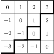
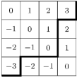
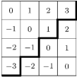
a	b	c

Figure 3. Admissible Sequence of Paths

Theorem 4.6.

Consider the maximal dominant weights $k\Lambda_{0}-\gamma_{\ell}\in\max(k\Lambda_{0})\cap P^{+},$ where $1\leq\ell\leq\lfloor\frac{n}{2}\rfloor$. The multiplicity of $k\Lambda_{0}-\gamma_{\ell}$ in $V(k\Lambda_{0})$ is equal to $|\mathcal{T}_{\ell}^{k}|$.

Proof.

It is enough to show that the elements in $\mathcal{T}_{\ell}^{k}$ are in one-to-one correspondence with the $k$-tuples of extended Young diagrams in $B(k\Lambda_{0})_{k\Lambda_{0}-\gamma_{\ell}}$.

Let $\mathbf{T}\in\mathcal{T}_{\ell}^{k}$ be an admissible sequence of $(k-1)$ paths. Recall that the paths in $\mathbf{T}$ are all drawn in an $\ell\times\ell$ square, $Y$. We construct the $k$-tuple $\mathbf{Y}=(Y_{1},\ldots,Y_{k})$ of extended Young diagrams as follows. First, we remove the boxes below $p_{1}$ and use these boxes to uniquely form an extended Young diagram of charge zero, which we will denote by $Y_{2}$. Next, we consider the boxes between $p_{1}$ and $p_{2}$ in $\mathbf{T}$. Since for $j>0,t_{3}^{j}\leq t_{3}^{j-1}\leq t_{3}^{j-2}\leq\ldots\leq t_{3}^{1}\leq t_{3}^{0}$ and for $j<0,t_{3}^{j}\leq t_{3}^{j+1}\leq t_{3}^{j+2}\leq\ldots\leq t_{3}^{-1}\leq t_{3}^{0}$ by Definition 4.4(2b), we can use these boxes to form a unique extended Young diagram $Y_{3}$ of charge zero. Now, by Definition 4.4(2a), $t_{2}^{j}\geq t_{3}^{j}$ for all colors $j$, which implies $Y_{2}\supseteq Y_{3}$. We continue this process until the boxes between $p_{k-1}$ and $p_{k-2}$ have been used to form the extended Young diagram $Y_{k}$, with $Y_{2}\supseteq Y_{3}\supseteq\ldots\supseteq Y_{k}$. The boxes above $p_{k-1}$ form an extended Young diagram, which we denote by $Y_{1}$. Since for each color $j$, $t_{i}^{j}\leq\ell-|j|-t_{2}^{j}-\sum_{a=2}^{i-1}t_{a}^{j}$, $3\leq i\leq k-1$ by Definition 4.4(2a), we have $Y_{1}\supseteq Y_{2}$. Note that $\mathbf{Y}$ has weight $k\Lambda_{0}-\gamma_{\ell}$ and that $\mathbf{Y}\in\mathcal{Y}(k\Lambda_{0})$. Now, consider each extended Young diagram as a sequence and use the notation $Y_{r}=(y_{i}^{(r)})_{i\geq 0},1\leq r\leq k$. We define $Y_{k+1}=Y_{1}[n]=(y_{i}^{(1)}+n)_{i\geq 0}$. Since $n\geq 2\ell$, we have $y_{i}^{(1)}+n>0$ for all $i\geq 0$. Note that by definition $(Y_{k})_{i}=y_{i}^{(k)}\leq 0$ for all $i\geq 0$. Hence for all $i\geq 0$, $(Y_{k+1})_{i}>(Y_{k})_{i+1}$ and $Y_{k}\supseteq Y_{1}[n]$. Therefore, by Theorem 4.2, $\mathbf{Y}\in B(k\Lambda_{0})_{k\Lambda_{0}-\gamma_{\ell}}$.

Now, let $\mathbf{Y}=(Y_{1},Y_{2},\ldots,Y_{k})\in B(k\Lambda_{0})_{k\Lambda_{0}-\gamma_{\ell}}$. Since $wt(\mathbf{Y})=k\Lambda_{0}-\gamma_{\ell}$, the total number of boxes in $\mathbf{Y}$ is $\ell^{2}$. We need to construct an admissible sequence $\mathbf{T}\in\mathcal{T}_{\ell}^{k}$ of $(k-1)$ lattice paths. We take $Y$ to be an empty diagram and fill it with the boxes in $\mathbf{Y}$ as follows, maintaining color positions as in Fig. 2. We begin by placing $Y_{1}$ in $Y$, aligning the upper left corners. Next, we draw a lattice path tracing the right edge of $Y_{1}$ from the lower left to upper right corner and take this path to be $p_{k-1}$. Now, we take the boxes from $Y_{k}$ and place them in $Y$, placing each box of color $j$ in the leftmost available position for that color. Since each $Y_{i},1\leq i\leq k$, is an extended Young diagram and since we have exactly $\ell-|j|$ boxes available of each color, we obtain an extended Young diagram. Thus, we are able to draw a lattice path along the right edge of the new diagram. We take this path to be $p_{k-2}$. Now, we add the boxes of $Y_{k-1}$ in the same manner and draw $p_{k-3}$. We continue this process until we add in the final boxes of $Y_{2}$ to make a complete square. Let $\mathbf{T}$ be the sequence of $k-1$ lattice paths in the square. As before, we define $t_{i}^{j}$ to be the number of $j$-colored boxes between $p_{i-1}$ and $p_{i-2}$. Notice that $t_{i}^{j}$ is the number of boxes of color $j$ in $Y_{i}$. Since each $Y_{i}$ is an extended Young diagram, Definition 4.4(2b) is satisfied. Since $Y_{1}\supseteq Y_{2}\supseteq\cdots\supseteq Y_{k}$, Definition 4.4(2a) and Definition 4.4(1) are satisfied. Hence $\mathbf{T}$ is an admissible sequence of $k-1$ lattice paths, which completes the proof.

∎

Example 4.7.

We associate the element of $\mathcal{T}_{4}^{3}$ in Fig. 4a with an element of $B(3\Lambda_{0})$ of weight $3\Lambda_{0}-\gamma_{4}$ as follows. First, we remove the boxes below and to the right of $p_{1}$ and obtain $Y_{1}$ as in Fig. 4b and $Y_{2}$ as the second element in Fig. 4c. Next, we remove the box that remains below $p_{2}$ to determine $Y_{3}$ as in Fig. 4c.

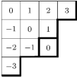
a	b
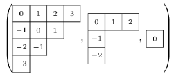
c

Figure 4. Correspondence Between Sequence of Admissible Paths and Element of $B(k\Lambda_{0})_{k\Lambda_{0}-\gamma_{\ell}}$

Corollary 4.8.

When $k=2$, the multiplicity of $2\Lambda_{0}-\gamma_{\ell}\in\max(2\Lambda_{0})\cap P^{+}$ is the number of lattice paths in an $\ell\times\ell$ square that must stay below, but can touch the diagonal $y=x$.

Denote a permutation of $\{1,2,\ldots n\}$ by a sequence $w=w_{1}w_{2}\ldots w_{n}$ indicating that $1\mapsto w_{1},2\mapsto w_{2},\ldots,n\mapsto w_{n}$. A $(j,j-1,\ldots,1)$-avoiding permutation is a permutation which does not have a decreasing subsequence of length $j$. For example, $w=1342$ is a 321-avoiding permutation because it has no decreasing subsequence of length three. Now we have the following conjecture.

Conjecture 4.9.

The multiplicities of the maximal dominant weights $(k\Lambda_{0}-\gamma_{\ell})$ of the $\widehat{sl}(n)$-modules $V(k\Lambda_{0})$ are given by mult${}_{k\Lambda_{0}}(k\Lambda_{0}-\gamma_{\ell})=\left|\{(k+1)(k)\ldots 21\text{-avoiding permutations of }[\ell]\}\right|.$

By definition, $T_{\ell}^{2}$ is the set of all lattice paths in an $\ell\times\ell$ square that do not cross $y=x$. As shown in ([2], page 361), there is a bijection between the lattice paths in $T_{\ell}^{2}$ and the set of 321-avoiding permutations of $\{1,2,\ldots,\ell\}$ as follows. Given $p\in T_{\ell}^{2}$ we construct a $321$-avoiding permutation $w=w_{1}w_{2}\ldots w_{\ell}$ of $[\ell]=\{1,2,\ldots,\ell\}$. As we traverse $p$ from $(0,0)$ to $(\ell,\ell)$, let $\{(v_{1},j_{1}),(v_{2},j_{2}),\ldots(v_{r},j_{r})\}$ be the coordinates at the top of each vertical move, not including $(\ell,\ell)$, which is at the top of the final vertical move. We define $w_{j_{i}}=v_{i}+1$ for $1\leq i\leq r$. The remaining $w_{i}$’s are defined by the unique map $\{1,2,\ldots,\ell\}\setminus\{j_{1},j_{2},\ldots,j_{r}\}\mapsto\{1,2,\ldots,\ell\}\setminus\{w_{j_{1}},w_{j_{2}},\ldots,w_{j_{r}}\}$ in increasing order. It follows from the construction that $w$ is a 321-avoiding permutation.

Conversely, let $w=w_{1}w_{2}\ldots w_{\ell}$ be a 321-avoiding permutation of $[\ell]$. Define $C_{i}=\{j\mid j>i,w_{j}<w_{i}\},c_{i}=|C_{i}|,$ and $J=\{j_{1}<j_{2}<\cdots<j_{r}\}=\{j\mid c_{j}>0\}$. We define a path, $p\in T_{\ell}^{2}$, from $(0,0)$ to $(\ell,\ell)$ by the moves given in Table 3.

Table 3. Rules for Drawing Lattice Path

Direction	From	To
Horizontal	$(0,0)$	$(c_{j_{1}}+j_{1}-1,0)$
Vertical	$(c_{j_{1}}+j_{1}-1,0)$	$(c_{j_{1}}+j_{1}-1,j_{1})$
Horizontal	$(c_{j_{1}}+j_{1}-1,j_{1})$	$(c_{j_{2}}+j_{2}-1,j_{1})$
Vertical	$(c_{j_{2}}+j_{2}-1,j_{1})$	$(c_{j_{2}}+j_{2}-1,j_{2})$
⋮	⋮	⋮
Horizontal	$(c_{j_{r}}+j_{r}-1,j_{r})$	$(\ell,j_{r})$
Vertical	$(\ell,j_{r})$	$(\ell,\ell)$

In the following two examples we illustrate this bijection. Thus Conjecture 4.9 is true for $k=2$. Furthermore, it is known (c.f. [6]) that the number of 321-avoiding permutations of $\{1,2,\ldots,\ell\}$ is equal to the $\ell^{th}$ Catalan number, which coincides with the result for the multiplicity of $2\Lambda_{0}-\gamma_{\ell}$ in [7].

Example 4.10.

Let $\ell=4$ and consider the 321-avoiding permutation $w=1342$. We obtain the values for $c_{i},i=1,2,3,4$ shown in Fig. 5a. Subsequently, we have the path coordinates in Fig. 5b, giving the path shown in Fig. 5c.

$i$ $C_{i}$ $c_{i}$ 1 - 0 2 4 1 3 4 1 4 0 0	Direction From To Horizontal $(0,0)$ $(2,0)$ Vertical $(2,0)$ $(2,2)$ Horizontal $(2,2)$ $(3,2)$ Vertical $(3,2)$ $(3,3)$ Horizontal $(3,3)$ $(4,3)$ Vertical $(4,3)$ $(4,4)$
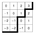
a	b	c

Figure 5. Data for the avoiding permutation 1342

Example 4.11.

Let $\ell=4$ and consider the admissible path in Fig. 6a. We wish to construct a 321-avoiding permutation $w=w_{1}w_{2}w_{3}w_{4}$ to correspond with the admissible path. For each vertical move in the path, we determine values $w_{i}$ as in Fig. 6b. We conclude that the path corresponds with the 321-avoiding permutation $w=3142$.

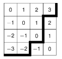
	Vertical Move Associated $w_{i}$ (2,1) $w_{1}=3$ (3,3) $w_{3}=4$ other $w_{2}=1$, $w_{4}=2$
a	b

Figure 6. Corresponding admissible path and avoiding permutation

In Table 4, using Theorem 4.6 we give the multiplicities of maximal dominant weights $k\Lambda_{0}-\gamma_{\ell}$ for $k\leq 9$ and $\ell\leq 9$. We observe that these multiplicities coincide with the number of $(k+1)(k)\ldots 21$-avoiding permutations of $\{1,2,\ldots,\ell\}$. For some partial results in the $k\geq 3$ case, see [3].

Table 4. Multiplicity Table for $k\Lambda_{0}-\gamma_{\ell}$

$k$	3	4	5	6	7	8	9
$\ell=2$	2	2	2	2	2	2	2
$\ell=3$	6	6	6	6	6	6	6
$\ell=4$	23	24	24	24	24	24	24
$\ell=5$	103	119	120	120	120	120	120
$\ell=6$	513	694	719	720	720	720	720
$\ell=7$	2761	4582	5003	5039	5040	5040	5040
$\ell=8$	15767	33324	39429	40270	40319	40320	40320
$\ell=9$	94359	261808	344837	361302	362815	362879	362880
$\ell=10$	586590	2190688	3291590	3587916	3626197	3628718	36228799

References

[1] Barshevsky, O., Fayers, M., Schaps, M.: A non-recursive criterion for weights of a highest-weight module for an affine Lie algebra, arXiv:1002.3457v6 [math.RT] (2011).
[2] Billey, S.C., Jockusch, W., Stanley, R.P.: Some Combinatorial Properties of Schubert Polynomials, J. Alg. Combin. 2 (1993) 345-374.
[3] Jayne, R.L.: Maximal dominant weights of some integrable modules for the special linear affine Lie algebras and their multiplicities. NCSU Ph.D. Dissertation. (2011).
[4] Jimbo, M., Misra, K.C., Miwa, T., Okado, M.: Combinatorics of representations of at , Commun. in Math. Phys. 136 (1991) 543-566.
[5]Kac, V.G.: Infinite-dimensional Lie algebras. Third edition. Cambridge University Press, New York, 1990.
[6] Stanley, R.P.: Enumerative Combinatorics. Vol. 2. Cambridge University Press, New York, 1999.
[7] Tsuchioka, S.: Catalan numbers and level 2 weight structures of , RIMS Kǒkyǔroku Bessatsu. B11 (2009) 145-154.