Probing quantum transport by engineering correlations in a speckle potential

Abstract

We develop a procedure to modify the correlations of a speckle potential. This procedure, that is suitable for spatial light modulator devices, allows one to increase the localization efficiency of the speckle in a narrow energy region whose position can be easily tuned. This peculiar energy-dependent localization behavior is explored by pulling the potential through a cigar-shaped Bose-Einstein condensate. We show that the percentage of dragged atoms as a function of the pulling velocity depends on the potential correlations below a threshold of the disorder strength. Above this threshold, interference effects are no longer clearly observable during the condensate drag.

I Introduction

The interplay between disorder and interactions in many-body systems gives rise to a remarkable richness of phenomena. In the absence of interactions, the presence of a random potential induces the suppression of wave propagation, as predicted by Anderson Anderson (1958, 1985). In Anderson localization, the waves diffracted by the impurities interfere destructively in the forward direction, with a resulting vanishing wave transmission and exponentially localized eigenstates. On the other hand, in the absence of disorder, interactions can induce localized states such as gap solitons Eiermann et al. (2004), and suppress transport as in the Mott regime Fisher et al. (1989).

If an interacting quantum gas is subjected to a disorder potential, exotic phases appear on lattice systems Fisher et al. (1989); Scalettar et al. (1991); Ristivojevic et al. (2012). In continuum systems, it was shown that disorder shifts the onset of superfluidity to lower Pilati et al. (2009); Allard et al. (2012) or larger Pilati et al. (2009) critical temperatures. In the superfluid regime, the presence of a random potential does not perturb the dynamics of the system in the low-energy regime. Indeed, below a critical velocity $v_{cr}$ that depends on the gas density and on the disorder strength Onofrio et al. (2000); Astrakharchik and Pitaevskii (2004); Ianeselle et al. (2006), the system, being superfluid, does not scatter against the potential defects. On the contrary, at velocities greater than $v_{cr}$, superfluidity breaks down and the interference of the scattered waves may deeply modify the system transport Paul et al. (2007, 2009) unto the Anderson localization regime.

The authors of Refs. Paul et al. (2007, 2009) studied the transport of a homogeneous one-dimensional (1D) interacting Bose-Einstein condensate (BEC) in the presence of a moving random potential of finite extent $L$. They proved the presence of an Anderson localization regime by studying the transmission of the BEC through the potential and showing that it decays exponentially with $L$. However, in ordinary ultracold-atom experiments, BECs are trapped in a harmonic confinements and thus they are inhomogeneous. Transmission is no longer a well defined observable in such a geometry, however one can identify the presence of some localization effects by studying the time evolution of the BEC center-of-mass Alamir et al. (2012, 2013). If the center-of-mass follows the moving random potential, the BEC is trapped by the random potential; it remains difficult to say if this localization is classical or induced by the interference of the scattered fluid.

In this paper we show that it is possible to enhance the role of interference in the localization process of an inhomogeneous interacting BEC by introducing tunable correlations in the disorder potential. Our reference potential is the speckle since it is the paradigm of the disordered potentials in ultracold atom experiments Clément et al. (2005); Billy et al. (2008); Kondov et al. (2011); Jendrzejewski et al. (2012); Shapiro (2012). The spectral function of a conventional speckle has a finite-$k$ support and decreases monotonically with the energy. In this work, we propose a novel speckle whose spectral function is also defined on a compact space but which posseses a narrow peak whose energy position is easily tuned by varying just one setup parameter. Our scheme, that is illustrated in Sec. II, can be straight implemented with a Spatial Light Modulator (SLM) device.

As shown in Sec. III, a peak in the spectral function results in a peak of the single-particle localization efficiency at a given energy, meaning that high-energy particles can be localized in a selective way. This is crucial in our setup where one needs to exceed the threshold $v_{cr}$ of the pulling velocity of the random potential to break down superfluidity and observe Anderson localization Paul et al. (2007, 2009). Thanks to the versatility of our potential, it is possible to drive the efficiency of the localization toward this energy range, and then to study the BEC localization as a function of the energy by varying the relative velocity between the BEC and the random potential. The observation of a localization peak in the expected energy range is a clear signature of the role of interference, and thus of the quantum nature, in the localization process of the boson gas.

The paper is organized as follows. In Sec. II the experimental proposal for the realization of our unconventional speckle is illustrated and its statistical properties are analyzed. The single-particle localization efficiency of a potential realized with this speckle is studied in Sec. III. In Sec. IV we introduce the time-dependent nonpolynomial nonlinear Schrödinger equation (NPSE) that describes the condensate dynamics in the elongated geometry and in the presence of a moving disorder potential. In Sec. V we show that the localization efficiency of the random potential depends on the correlations of the potential only at small values of the disorder strength. At larger potential strength, the percentage of localized atoms is no longer sensitive to the microscopic details of the disorder: the BEC is just classically trapped by the potential wells. Our concluding remarks are given in Sec. VI.

II Speckle potential with tunable correlations

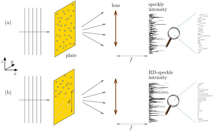
Figure 1: (Color online) Schematic representation of the device allowing tunable correlations in the speckle: an incident plane wave is diffracted by a plate with a random distribution of holes. The diffraction pattern obtained in the focal plane of a converging lens is a standard speckle if the hole distribution is $\delta$-correlated (a), while it is a RD-speckle if the hole distribution is dimerized in the $z$ direction (b). In the plate in the bottom row, the different borders of the hole (black continuous line and red dotted line) are a guide for the eyes to identify the dimerization of the hole distribution.

To generate a speckle, we consider the set-up illustrated in Fig. 1(a). An incident plane wave of wavelength $\lambda_{L}$ is diffracted by a matte square plate of side $L$ covered with a random distribution of $N_{h}$ identical holes of radius $r$. The Fraunhofer diffraction pattern obtained in the focal plane of a converging lens of focal length $f$ is given by

$$I(y,z)=I_{h}(y,z)\left|\sum_{i=1}^{N_{h}}e^{-\frac{2i\pi}{\lambda_{L}f}(yy_{i}+zz_{i})}\right|^{2}$$ (1)

where $I_{h}(y,z)$ is the diffraction pattern of a single hole, and $\{y_{i},z_{i}\}$ are the coordinates of the $i$-th hole. If $I_{h}(y,z)$ is constant in the scanned spatial region ($r$ is small enough), and if the hole distribution is $\delta$-correlated, $I(y,z)$ (excluding the region around $y=0$ and $z=0$) is a standard speckle with the two-point correlation function $C(\delta y,\delta z)=\langle I(y,z)I(y+\delta y,z+\delta z)\rangle-\langle I\rangle^{2}$ given by

$$C(\delta y,\delta z)=\langle I\rangle^{2}\,{\rm sinc}^{2}\left(\dfrac{L\,\delta y}{\lambda_{L}f}\right){\rm sinc}^{2}\left(\dfrac{L\,\delta z}{\lambda_{L}f}\right),$$ (2)

where $\langle\rangle$ denotes both the average over disorder realizations and over each realization. This is shown in Fig. 2 in red dotted line where we have plotted the rescaled correlation function $c(\delta z)=C(0,\delta z)/C(0,0)$ (top panel) and the corresponding spectral function

$$S(q)=\int_{-\infty}^{+\infty}e^{-i2\pi q\delta z}c(\delta z)\,d(\delta z),$$ (3)

that is the well-known triangular function that goes to zero at $q=1/\sigma_{R}$, $\sigma_{R}=(\lambda_{L}f)/L$ being the correlation length (bottom panel). The compact-$q$ support of the speckle is a result of the finite size of the diffracting plate. These results were obtained numerically from the random potentials used in the dynamical simulations of Sec. IV.

The speckle properties are robust to short-distance correlations in the hole distribution when the correlation range is much smaller than the plate size Goodman (2007). But by introducing hole correlations at larger distances, $c(\delta z)$ and $S(q)$ can be accordingly modified. In particular we consider a hole-dimerized distribution, where at each hole at position $\{y_{i},z_{i}\}$ corresponds another hole at position $\{y_{i},z_{j}\}$ with $y_{j}=y_{i}$ and $|z_{j}-z_{i}|=d$ (see Fig. 1(b)). From a distance the resulting speckle looks similar to the standard one, but by zooming in the presence of some order in the grain distribution is clearly observable. Indeed, the resulting light pattern, for the case $d<L/2$ where each hole has a partner at a distance $d$,

$$\begin{split}I_{RD}(y,z)&\propto\left|\sum_{i=1}^{N_{h}/2}[e^{-\frac{2i\pi}{\lambda_{L}f}(yy_{i}+zz_{i})}+e^{-\frac{2i\pi}{\lambda_{L}f}(yy_{i}+z(z_{i}+d))}]\right|^{2}\\ &=\left|\sum_{i=1}^{N_{h}/2}e^{-\frac{2i\pi}{\lambda_{L}f}(yy_{i}+zz_{i})}\right|^{2}\{2\cos[\pi zd/(\lambda_{L}f)]\}^{2}\\ \end{split}$$ (4)

is a product of the standard speckle and a sinusoidal function with the spatial period $\lambda_{L}f/d$. The correlation function of such a random-dimer speckle (RD-speckle) corresponds roughly to the superposition of the correlation function for a standard speckle and a sinusoidal function with a well-defined spatial frequency (see top panel of Fig. 2), that results in a peak at $q=d/(L\sigma_{R})$ in the corresponding spectral function (bottom panel).

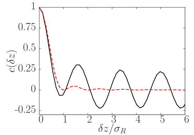
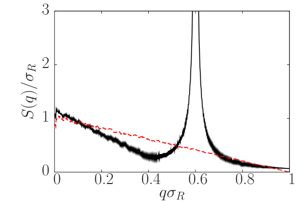
Figure 2: (Color online) Rescaled correlation function $c(\delta z)$ as a function of $\delta z$ in unit of $\sigma_{R}$ (top panel) and spectral function $S(q)$ (in units of $\sigma_{R}$) as a function of $q$ in unit of $1/\sigma_{R}$ (bottom panel) for the case of a standard speckle (dashed-red line) and a RD-speckle (continuous-black line). We set $L=2$ cm, $\lambda_{L}=532$ nm, $f=2.3$ cm, $d=1.20$ cm, and $N_{h}$ is of the order of 100. The results were calculated from the random potentials of finite extent used in the dynamical calculations of Sec.  IV, averaging over 500 configurations.

For the case $d\geq L/2$ few holes located at the plate center have no partners. We have checked that these few holes do not affect the spectral function with respect to a case where all holes are dimerized.

Although correlations in the speckle have been previously introduced by changing the aperture of the diffusive plate or the spatial profile of the incident beam as proposed in Refs. Piraud et al. (2012); Płodzień and Sacha (2011); Piraud and Sanchez-Palencia (2013), and other strategies have been proposed in the context of microwave experiments to introduce a non-monotonic behaviour of the localization efficiency Izrailev and Krokhin (1999); Kuhl et al. (2008), the interest of the present RD-speckle lies in the possibility to control the position of the peak in the spectral function $S(q)$ with standard experimental techniques. As it will be enlightened in the following, this property allows to scan, as a function of the energy, the response of a system to the disorder potential generated by the light pattern. Indeed the standard speckle and the RD-speckle can be used as disorder potentials in an ultracold-atom experiment, the strength of the potentials being given by

$${\mathscr{V}}(y,z)\simeq-I(y,z)\frac{3\pi c_{\text{light}}^{2}}{2\omega_{at}^{3}}\frac{\Gamma}{\delta}$$ (5)

where $c_{\text{light}}$ is the light velocity, $\Gamma$ the linewidth of the atomic transition, $\delta=\omega_{at}-\omega_{L}$ the detuning between the atomic frequency $\omega_{at}$ and the laser frequency $\omega_{L}=2\pi c_{\text{light}}/\lambda_{L}$. Furthermore, as in the Born approximation the spectral function $S(q)$ is proportional to the inverse of the localization length, by changing the correlation properties of the speckle one effectively modifies the localization in the same manner.

The geometry of the random potential ${\mathscr{V}}(y,z)$ can be varied by changing the dimensions of the plate. A 1D random potential Billy et al. (2008) can be realized for instance by squeezing the $y$-size of the diffusive plate. In this way, the transverse size of the speckle grains can be much larger than the system transverse size. This is equivalent to considering the 1D potential $V(z)={\mathscr{V}}(y=\bar{y},z)$ as it will be done in the following.

III Single-particle localization efficiency

With the aim to clarify the effects of a RD-speckle potential in the Anderson localization frame, we study the propagation of a quantum particle of mass $m$ along an infinitely long 1D disorder potential $V(z)$, as described by the time-independent Schrödinger equation

$$-\frac{\hbar^{2}}{2m}\frac{\partial^{2}}{\partial z^{2}}\psi(z)+V(z)\,\psi(z)=E\psi(z),$$ (6)

$E=\hbar^{2}k_{E}^{2}/2m+\langle V\rangle$ being the particle energy. The Lyapunov exponent $\gamma(E)$ that coincides with the inverse of the localization length $\mathcal{L}_{loc}(E)$, is given by Paladin and Vulpiani (1987)

$$\gamma(E)=\dfrac{1}{\mathcal{L}_{loc}(E)}=\lim_{|z|\rightarrow\infty}\frac{1}{|z|}\left\langle\ln\left(\frac{k^{2}_{E}\psi^{2}(z)+\psi^{\prime 2}(z)}{k^{2}_{E}\psi^{2}(0)+\psi^{\prime 2}(0)}\right)\right\rangle.$$ (7)

We compute numerically $\gamma(E)$ by discretizing the Schrödinger equation on a spatial grid and writing the equation in a matrix form:

$$\begin{pmatrix}&\psi_{n+1}\\ &\psi_{n}\end{pmatrix}=T_{n}\begin{pmatrix}&\psi_{n}\\ &\psi_{n-1}\end{pmatrix}$$ (8)

where $\psi_{n}$ is the wave function at the grid position $n$ and $T_{n}$ is a so-called transfer matrix. The final wave vector $(\psi_{n+1},\psi_{n})^{T}$ is found by plugging in an initial vector $(\psi_{1},\psi_{0})^{T}$ and solving recursively Eq. (8). We used as initial wave $(\psi_{0},\partial_{z}\psi_{0})=(1,k/\tan\theta)$ where $\theta\in[0,2\pi]$ is a random angle Piraud (2012) and we exploited the Numerov algorithm Chow (1972) to write Eq. (8) at each spatial point. We propagated the wave over a grid of $4\times 10^{6}$ points with step size 0.1$\sigma_{R}$, such that the details of the speckle function are taken into account, and averaged over $10^{4}$ realizations.

In Fig. 3 we show the behavior of $\gamma(E)$ as a function of $k_{E}$ for the case of a ⁸⁷Rb atom ($\lambda_{at}=2\pi c_{\text{light}}/\omega_{at}=780$ nm and $\Gamma=2\pi\times 6.065$ MHz) subjected to a disorder potential of strength $V_{dis}=\sqrt{\langle V^{2}\rangle}=0.117\,\hbar^{2}/m\sigma_{R}^{2}$, generated by a laser of wavelength $\lambda_{L}=532$ nm. We compare the case of a standard speckle (continuous black line) with that of a RD-speckle for different values of $d$. As shown for the spectral function $S(q)$ (Fig. 2), in the RD case a peak appears whose position depends linearly on $d$ (dashed, dotted and dot-dashed lines in Fig. 3). Thus the RD-speckle potential allows to achieve and control the localization of high-energy atoms.

Except for the main peak, $\gamma(E)$ of the RD-speckle has the same trend as the conventional speckle displaying the effective mobility edge at $k_{E}=\pi/\sigma_{R}$ Lugan et al. (2009). This was predictable from the calculation of the spectral function $S(q)$ (see bottom panel of Fig. 2) since the Lyapunov coefficient evaluated in the Born approximation is proportional to $S(2q)$ and $k_{E}=2\pi q$. The overall behavior of the RD-speckle is clearly observable in the inset of Fig. 3 where we have plotted $\gamma(E)$ using a logarithmic scale and over a larger range of $k_{E}$. In particular, we observe several low amplitude revivals at higher energies located at integer multiples of the position of the main peak.

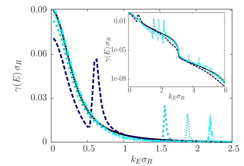
Figure 3: (Color online) Lyapunov exponent $\gamma(E)$ in unit of $1/\sigma_{R}$ as a function of $k_{E}\sigma_{R}$ for a standard speckle potential (continuous black line) and for RD-speckle potentials with $d=0.4,1,1.2$ and $1.4$ cm (colored dashed lines) from left to right. The inset shows the same curve but in log-scale, over a wider $k_{E}$ range.

IV Dynamics of a quasi-one dimensional BEC

We study the dynamics of a system of $N=10^{5}$ Bose-Einstein condensed ⁸⁷ Rb atoms of mass $m$ subject to a static cigar-shaped harmonic trap and a time-dependent random potential:

$$U(\textbf{r},t)=\frac{1}{2}m\omega^{2}_{\perp}(x^{2}+y^{2})+\frac{1}{2}m\omega^{2}_{z}z^{2}+V(z,t)$$ (9)

with $\omega_{\perp}=2\pi\times 235.8$ Hz and $\omega_{z}=2\pi\times 22.2$ Hz the trapping frequencies in the perpendicular and longitudinal directions, respectively. The last time-dependent term in (9) corresponds to a random potential that is fixed in the moving frame $z^{\prime}=z-vt$, ${\bf v}=v\hat{e}_{z}$ being the drift velocity. The random potential is generated by the procedure illustrated in Sec. II.

Under cigar-shaped trap geometry, the full 3D equation of motion for the BEC wavefunction $\psi(\textbf{r},t)$ can be reduced to the effective 1D time-dependent nonpolynomial nonlinear Schrödinger equation (NPSE) Salasnich et al. (2002)

$$\begin{split}i\hbar\frac{\partial}{\partial t}f&=\left[-\frac{\hbar^{2}}{2m}\frac{\partial^{2}}{\partial z^{2}}+\frac{1}{2}m\omega^{2}_{z}z^{2}+V(z,t)\right.\\ &\left.+\hbar\omega_{\perp}\frac{1+3a_{s}N|f|^{2}}{\sqrt{1+2a_{s}N|f|^{2}}}\right]f.\end{split}$$ (10)

with $a_{s}$ being the s-wave scattering length that we set at $80a_{B}$ and $a_{B}$ being the Bohr radius. To obtain Eq. (10) we set

$$\psi(\textbf{r},t)=f(z,t)\phi(\textbf{r},t)=f(z,t)\frac{e^{-(x^{2}+y^{2})/2\sigma^{2}(z,t)}}{\sqrt{\pi}\sigma(z,t)}$$ (11)

where the transverse part $\phi(\textbf{r},t)$ is modeled by a Gaussian function with variance $\sigma(z,t)$. Within the assumption that this variance varies slowly as functions of $z$ and $t$, $\sigma(z,t)$ is given by

$$\sigma^{2}(z,t)=\ell_{0}^{2}\sqrt{1+2a_{s}N|f(z,t)|^{2}},$$ (12)

where $\ell_{0}=\sqrt{\hbar/(m\omega_{\perp})}$ is the oscillator length in the transverse direction. The 3D density profile is then

$$\rho(\textbf{r})=\tilde{\rho}(z)\frac{e^{-(x^{2}+y^{2})/\sigma^{2}}}{\pi\sigma^{2}},$$ (13)

with $\tilde{\rho}(z)=|f|^{2}$ the integrated 1D density.

The NPSE is numerically solved using a split-step method and spatial Fast Fourier transforms (FFT). First we compute the equilibrium density profile in the presence of a static disorder potential. Then, we switch on the drift velocity $v$ and compute the time evolution of the condensate wavefunction $f(z,t)$.

V Quantum versus classical transport

The scheme of the proposed experiment is the following. The disorder potential is pulled through the BEC with a velocity $v$ over a distance $L^{*}$. We measure the center-of-mass shift $z_{cm}$ and we identify the ratio of localized atoms $N_{loc}/N$ with the ratio $z_{cm}/L^{*}$, indeed if the whole BEC is insensible to the disorder potential then $z_{cm}=0$, while if the whole BEC is stuck on the disorder potential then $z_{cm}=L^{*}$ Alamir et al. (2012).

Since we expect to observe localization for $v\gtrsim c$, $c=\sqrt{\mu/2m}$ being the 1D speed of sound Paul et al. (2009); Albert et al. (2010); Alamir et al. (2012) with $\mu$ the chemical potential, we tune the position of the localization peak in this region and choose the value of the dimer length $d$ to enhance the interference effects. With this purpose, we study the localized BEC fraction $N_{loc}/N$ as a function of $v/c$ for the case of a RD-speckle of potential strength $V_{dis}=0.05\,\hbar\omega_{\perp}$ and different values of $d$, $d=0.4$ cm (blue circles), $d=0.8$ cm (turquoise crosses) and $d=1.2$ cm (black plus signs). This is shown in Fig. 4 where we can observe that the best resolved peak corresponds to $d=1.2$ cm. By identifying the drift velocity $v$ with $\hbar k_{E}/m$, this corresponds to a $\gamma(E)$ peak at $v\simeq 1.1c$.

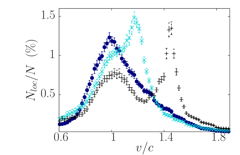
Figure 4: (Color online) Localized BEC fraction as a function of $v/c$ for the case of a RD-speckle with $d=0.4$ cm (blue circles), $d=0.8$ cm (turquoise crosses) and $d=1.2$ cm (black plus signs).

Here and in the following we average over 30 configurations; in all simulations we fix $L^{*}\simeq 56\sigma_{R}$, value that corresponds to $\sim 1.4$ times ${\mathcal{L}}_{loc}$ evaluated at the peak position of the case $d=1.2$ cm, which is the $d$ value that we set from now on.

The localized BEC fraction as a function of $v/c$ is shown in Fig. 5 for different values of the potential strength $V_{dis}$ for the case of a standard speckle (red squares) and a RD-speckle (black crosses).

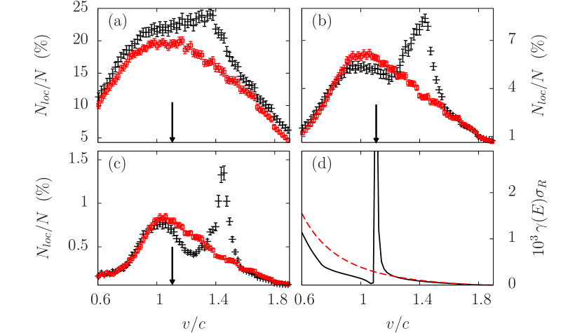
Figure 5: (Color online) Panels (a-c): localized BEC fraction as a function of $v/c$ for the case of a standard speckle (red square) and of a RD-speckle (black crosses). (a) $V_{dis}=0.39\,\hbar\omega_{\perp}$, (b) $V_{dis}=0.16\,\hbar\omega_{\perp}$ and (c) $V_{dis}=0.05\,\hbar\omega_{\perp}$. The vertical arrows indicate the position of the $\gamma(E)$ peak. Panel (d): $\gamma(E)$ in units $1/\sigma_{R}$ as a function of $v/c$ with $v=\hbar k_{E}/m$ for the standard speckle (dashed lines) and RD speckle (solid lines). All calculations correspond to $d=1.2$ cm.

We observe that at large values of $V_{dis}$, the behaviors of $N_{loc}/N$ of the standard and the RD speckles are quite similar (panel (a) of Fig. 5). By lowering $V_{dis}$, the global localization efficiency of the disorder potential decreases but a peak appears at $v/c\simeq 1.4$ for the case of a RD-speckle (panels (b) and (c) of Fig. 5), as already outlined in Fig. 4. Moreover this peak is preceded by a strong inhibition of the localization with respect to the standard speckle in agreement with the behaviour of $\gamma(E)$ (panel (d) in Fig. 5) where the curves for the standard and the RD speckles intersect before the peak.

Although the peak in $N_{loc}/N(v)$ can be attributed to the interference effects giving rise to the one of $\gamma(E)$, its position is shifted and the shape broader. Indeed the calculation of $\gamma(E)$ is done in the single-particle approximation for a steady potential, while the BEC is an inhomogeneous and interacting many-particle system. The system is then continuously disturbed by pulling the disorder potential; thus many factors may contribute to the shift and the broadening of the peak. We can also observe that the peak widens by increasing the disorder strength $V_{dis}$.

The behavior of the $N_{loc}/N$ peak for the RD-speckle as a function of $V_{dis}$ is shown in Fig. 6. In this figure we have plotted the visibility $\mathcal{V}$ of the peak, defined as

$$\mathcal{V}=\dfrac{\left(\dfrac{N_{loc}}{N}\right)_{\max}-\left(\dfrac{N_{loc}}{N}\right)_{\min}}{\left(\dfrac{N_{loc}}{N}\right)_{\max}+\left(\dfrac{N_{loc}}{N}\right)_{\min}}$$ (14)

where $\left(N_{loc}/N\right)_{\max}$ and $\left(N_{loc}/N\right)_{\min}$ are respectively the peak and the hollow preceding the peak of the function $\left(N_{loc}/N\right)(v/c)$.

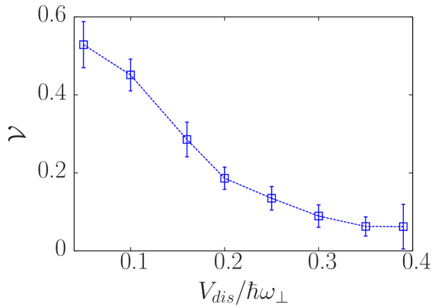
Figure 6: (Color online) Visibility $\mathcal{V}$ of the peak of the function $N_{loc}/N$ as a function of $V_{dis}$ in unit of $\hbar\omega_{\perp}$. The line is a guide to the eye.

For all values of $V_{dis}$ considered in Fig. 6, the chemical potential $\mu$ is of the order of $7.8\hbar\omega_{\perp}$, and thus the drift kinetic energy at the peak location ($v\simeq 1.4\,c$) is of the order of $2\mu\simeq 15.6\,\hbar\omega_{\perp}$ a quite large value with respect to the potential strengths $V_{dis}$ considered in this work. However in the standard speckle, as well as in the RD-one, the probability for high-intensity grains is not vanishing and the BEC can be trapped by few potential wells to quite low values of $V_{dis}$ as it happens for the case $V_{dis}=0.39\,\hbar\omega_{\perp}$ (panel (a) of Fig. 5). Moreover, because of the sinusoidal function [see Eq. (LABEL:newspeck)] that modulates the standard speckle on a smaller scale with respect the size grains, the probability to have very high grains is larger for the RD-speckle than for the standard speckle. This explains the fact that at $V_{dis}=0.39\,\hbar\omega_{\perp}$, the localization efficiency of the RD-speckle is larger than that of the standard speckle over the whole $v/c$ range. In order to observe interference effects in the localization dynamics, one needs to reduce $V_{dis}$ further so that to decrease the probability to have speckle grains over a given threshold. Indeed the peak in the $N_{loc}/N$ function becomes clearly visible ($\mathcal{V}\geq 0.2$) at $V_{dis}\leq 0.16\hbar\omega_{\perp}$.

For a better understanding of the role of the interactions on the peak distorsion and, more generally, on the localization efficiency, we vary the scattering length $a_{s}$ from 10 to 320 $a_{B}$ for fixed potential strength $V_{dis}=0.05\,\hbar\omega_{\perp}$. Let us remark that this is just a conceptual experiment since the ⁸⁷Rb scattering length cannot be tuned by exploiting Feshbach resonances. The results are shown in the top panel of Fig. 7, where we have drawn the localization efficiency for different interaction strengths as a function of $v/c$, $c$ being the sound velocity for the case $a_{s}=80a_{B}$ in order to fix the same velocity scale for all curves.

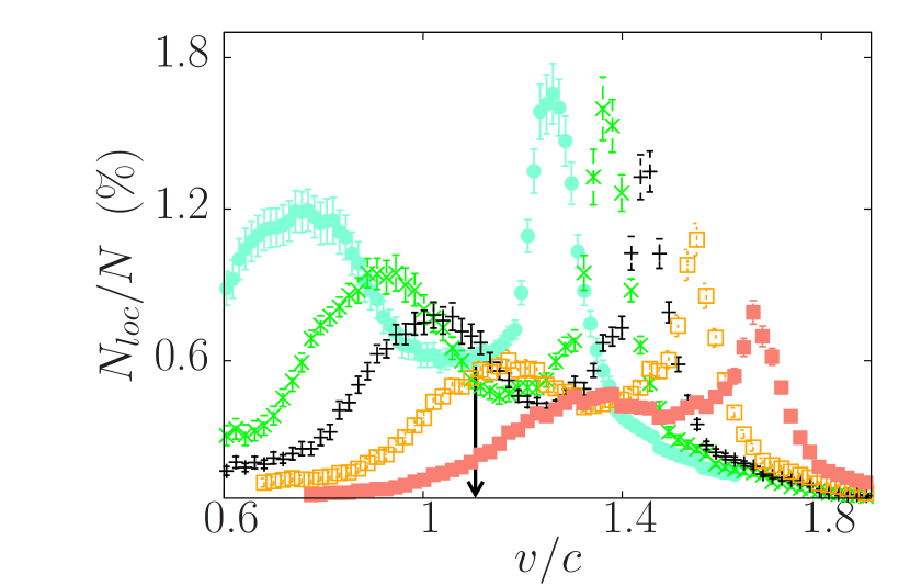
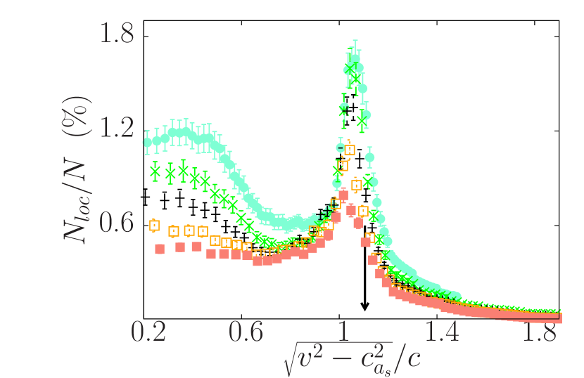
Figure 7: (Color online) Top panel: Localized BEC fraction as a function of $v/c$ ($c$ being the sound velocity for the case $a_{s}=80a_{B}$) for the case of a RD-speckle with $d=1.2$ cm and $V_{dis}=0.05\,\hbar\omega_{\perp}$. The different symbols correspond to $a_{s}=10a_{B}$ (aquamarine filled circles), $40a_{B}$ (green crosses), $80a_{B}$ (black plus signs), $160a_{B}$ (orange empty squares) and $320a_{B}$ (pink filled squares). The vertical arrows indicate the position of the $\gamma(E)$ peak. For each value of $a_{s}$ we average over 30 configurations. Bottom panel: The same as in the top panel, but the localized BEC fraction is shown as a function of $\sqrt{v^{2}-c_{a_{s}}^{2}}/c$, with $c_{a_{s}}$ being the sound velocity for the corresponding $a_{s}$.

The first observation is that the larger the value of the interaction is, the greater the shift of the position of the peak is. Indeed, in the presence of interactions, what really matters is the available kinetic energy $\frac{1}{2}mv^{2}-\frac{1}{2}mc_{a_{s}}^{2}$ Leboeuf and Pavloff (2001), where $c_{a_{s}}$ is the sound velocity corresponding at the scattering length $a_{s}$. Actually, if we plot $N_{loc}/N$ as a function of $\sqrt{v^{2}-c_{a_{s}}^{2}}/c$ (bottom panel of Fig. 7), all the peaks collapse at the same point, very close to the position of the $\gamma(E)$ peak. The second observation is that, by increasing interactions, the localization efficiency of the RD-speckle decreases overall in the $v$ space. By increasing the interactions we increase the robustness of the superfluidity, and the disorder potential becomes less and less efficient to localize the atoms. Indeed, if we consider, for example, the case $a_{s}=320a_{B}$ the position of the $\gamma(E)$ peak in units of $v/c_{320}$, $c_{320}$ being the corresponding sound velocity, we find $\sim 0.8v/c_{320}$ and thus is not the best value of $v$ for this scattering length. Therefore, to increase the efficiency of our potential at large interaction strengths, we should increase the value of $d$.

Finally we would like to stress that the measure of $N_{loc}/N$ by means of the center-of-mass shift is really a good observable to detect localization in a trapped system, both for the standard speckle and for our new proposed speckle. Indeed its statistical distribution function displays the expected behavior in the presence of localization.

Figure 8: (Color online) Statistical distribution $p(N_{loc}/N)$ for the RD-speckle with $V_{dis}=0.16\hbar\omega_{\perp}$, $d=1.2$ cm and for two values of $v$.

This is shown in Fig. 8 where we compare the statistical distribution $p(N_{loc}/N)$ for a RD speckle at two drift velocities. We observe that at the velocity corresponding to the localization maxima (left panel) the statistical distribution becomes rather symmetric as opposed to the shape for the larger $v$. This is in analogy to the behaviour of the transmission in a non-interacting homogeneous system Müller and Delande (2010), where one could expect a transition from a decreasing exponential distribution at vanishingly low localization ratio to a log-normal distribution when localization dominates. A complete analysis on this matter requires a thorough study entailing a systematic calculation of the statistical properties of the potential for many realizations, drift velocities, distances $d$, etc and therefore is left for future investigations.

VI Conclusions

We studied the dragging of a Bose-Einstein condensate of ⁸⁷Rb atoms confined in cigar-shaped traps in the presence of a correlated speckle potential. By constructing a speckle out of randomly distributed dimerized holes, we are able to select a non-vanishing energy value that maximizes the localization efficiency and thus to localize higher-energy atoms. Our approach can be implemented by spatial light modulator devices available as standard experimental equipment. By numerically solving the dynamics of the condensate subjected to an underlying disorder potential moving at constant speed, we have shown the efficacity and versatility of such a potential. By analyzing the center-of-mass displacement, we find that correlations enhance the localization by a factor of 2-3 with respect to standard speckle. The magnitude of this effect is very sensitive to the interaction strength and the amplitude of the disorder. Indeed a strong disorder inhibits interference thwarting the presence of correlations in the condensate dynamics.