Microscopic identification of dissipative modes in relativistic field theories

Abstract

We present an argument to support the existence of dissipative modes in relativistic field theories. In an $O(N)$ $\varphi^{4}$ theory in spatial dimension $d\leq 3$, a relaxation constant $\Gamma$ of a two-point function in an infrared region is shown to be finite within the two-particle irreducible (2PI) framework at the next-leading order (NLO) of $1/N$ expansion. This immediately implies that a slow dissipative mode with a dispersion $p_{0}\sim i\Gamma{\boldsymbol{p}}^{2}$ is microscopically identified in the two-point function. Contrary, NLO calculation in the one-particle irreducible (1PI) framework fails to yield a finite relaxation constant. Comparing the results in 1PI and 2PI frameworks, one concludes that dissipation emerges from multiple scattering of a particle with a heat bath, which is appropriately treated in the 2PI-NLO calculation through the resummation of secular terms to improve long-time behavior of the two-point function. Assuming that this slow dissipative mode survives at the critical point, one can identify the dynamic critical exponent $z$ for the two-point function as $z=2-\eta$. We also discuss possible improvement of the result.

I Introduction

It is generally a non-trivial and difficult challenge to deduce from a microscopic theory hydrodynamic behavior at long-time scales. As was clearly stated by Kadanoff and Martin Kadanoff and Martin (1963), it is because “hydrodynamic equations only appear when the behavior is dominated by the secular effects of collisions” and thus “most straightforward techniques for determining the correlation functions cannot be successfully applied”. In the present paper, we will demonstrate in a concrete model that the two-particle irreducible (2PI) framework which appropriately deals with secular effects through resummation is indeed able to describe the hydrodynamic behavior from the microscopic level, in particular, a dissipative mode in a two-point correlation function.

There are three different levels of descriptions for long-time (and long-distance) behavior of a locally equilibrated system. At time scales much longer than the correlation time (typical time scale of the system), hydrodynamics is established as the framework for time evolution of conserved densities through macroscopic variables such as temperature, chemical potentials and flow velocities. Diffusion and viscosity constants are regarded as low-energy effective constants. When we study (e.g.) temperature or momentum dependence of the low-energy constants, we need to include fluctuations around hydrodynamic behavior by employing a “meso-scopic” effective theory. The Mode-Coupling Theory (MCT) Halperin and Hohenberg (1967, 1969); Kawasaki (1970); Hohenberg and Halperin (1977) as a typical example, separates the slow and fast degrees of freedom and describes effective dynamics of the slow modes with treating effects of the fast modes as stochastic noise and bare parameter constants. In particular, non-conserved variables such as an order parameter field $\varphi$ may be included in addition to hydrodynamic modes in MCT when they contribute to slow dynamics of interest. Only after the microscopic theory is solved, all the phenomenological parameters would be fixed, which is the third level description. However, such a microscopic approach, if applied naively, is suitable only for short time description but starts to lose its accuracy at time scales longer than typical scattering time.

It should be also noticed that hydrodynamics applies at the scale much longer than the correlation length $\xi$ and therefore breaks down as the system approaches a critical point, where $\xi\to\infty$. MCT was originally devised to describe the slow dynamics near the critical point by including the order-parameter fluctuations $\varphi$ as well as those of conserved densities, and it is successful to reproduce the singularity of the transport coefficients as the critical point is approached. Accordingly MCT gives empirical values for the dynamic critical exponent $z$, which characterizes the dissipation time of a disturbance as $\tau\sim\xi^{z}$. Such a process should be associated with a dissipative mode whose dispersion is given by $p_{0}\propto i|{\boldsymbol{p}}|^{z}$ with $p_{0}$ and ${\boldsymbol{p}}$ the mode energy and momentum. The central problem of this paper is how to identify this dissipative mode by analyzing the two-point function of a microscopic theory.

Considering that MCT is just a phenomenological theory and that the dissipative mode (at the critical point) should couple in the two-point function of the order-parameter field $\varphi$, it is preferable if we can investigate the low-frequency behavior of the two-point function at the microscopic level. As far as we know, the 2PI approach Luttinger and Ward (1960); Cornwall et al. (1974); Berges (2005) is the only framework which allows us to describe the two-point function at the microscopic level, and making the secular effects from multiple scattering of particles tractable through resummation. This motivated us to work on the two-point function of $\varphi$ in the 2PI framework.

Recently, the 2PI effective action has been actively applied to non-equilibrium phenomena. One of the merits of the 2PI framework is that it treats, in addition to a condensate $\phi=\left<\varphi\right>$, the two-point correlation function of fluctuations $G=\left<\delta\varphi\delta\varphi\right>$ with $\delta\varphi=\varphi-\phi$ in a self-consistent way, and that we can systematically resum higher-order diagrams for $\phi$ and $G$ keeping conservation laws of the system preserved Baym and Kadanoff (1961); Baym (1962); Kadanoff and Baym (1962). Therefore, the 2PI framework is expected to be useful in describing time evolution of conserved densities, and thus in describing long-time evolution of the system.

In the present paper, we work on a relativistic $O(N)$ $\varphi^{4}$ scalar theory. Another motivation for our study is to see how a dissipative mode appears in the microscopic two-point function of a relativistic field theory . There is a controversial situation concerning the dynamic critical exponent $z$ between relativistic and nonrelativistic scalar theories. Analysis of the two-point function in a nonrelativistic $O(N)$ model Abe (1974); Abe and Hikami (1974) predicts $z$ close to 2, while a relativistic model gives different values for $z$ depending on the calculation methods: Dynamic renormalization group Boyanovsky et al. (2001); Boyanovsky and de Vega (2003) gives $z\sim 1$ while numerical simulation Berges et al. (2010) gives $z\sim 2$. In fact, as is shown in the present paper, these analyses of the two-point function of $\varphi$, except for the last numerical one, do not give us the exponent $z$ of a purely dissipative mode, but of the bare propagating modes, which decay much faster than dissipative modes. The dissipative mode emerges in the two-point function of $\varphi$ non-perturbatively only after the resummation. We will clarify these points in the text.

Before closing Introduction, let us list up several physical situations whose hydrodynamics are of interest. First, hydrodynamic picture is widely applied to describing long-time and long-distance behavior of various systems from Quark-Gluon Plasma (QGP) in heavy-ion collisions Kolb and Heinz (2004); Hirano et al. (2010); Hirano (2011) and Bose-Einstein condensate of cold atomic gas Stringari (1996), to astrophysical phenomena such as supernova explosions Takiwaki et al. (2012), and even to the universe itself Weinberg (1972). In particular, a critical point is conjectured in the QCD phase diagram, where the transition from hadronic degrees of freedom to QGP is of the 2nd order, and heavy-ion collision experiments for the critical point survey have already started Odyniec (2010); Mohanty et al. (2011). Locating the critical point on the QCD phase diagram is one of the main objectives in QGP physics now, and to this end we obviously need correct understanding of the dynamics near the critical point. There are indeed several works applying MCT to the critical dynamics of QCDRajagopal and Wilczek (1993); Fujii (2003); Fujii and Ohtani (2004); Son and Stephanov (2004); Ohnishi et al. (2005); Nakano et al. (2012). However, it is still controversial in the sense which hydrodynamic mode dominates the critical dynamics. Note also that people are trying to describe non-equilibrium phenomena from microscopic theories by exploiting the 2PI framework. For example, people discuss the problem of how QGP can be formed within a short time after heavy-ion collisions Berges et al. (2009, 2013); Dusling et al. (2012); Epelbaum and Gelis (2013) and also non-equilibrium phenomena in cold atomic systems Gasenzer (2009). We hope that fundamental understanding on the dissipative modes in the present paper would be helpful for various phenomena including the QGP physics.

This paper is organized as follows: In Section 2, we discuss how a dissipative mode emerges from a two-point correlation function using both 1PI and 2PI effective actions. In particular, we focus on the way how the effects of multiple scattering with a heat bath is included, and propose a criterion for the emergence of a dissipative mode. In Section 3, we check the criterion in $O(N)$-symmetric $\varphi^{4}$ model within two different ways of calculations: 1PI and 2PI frameworks. We will find that the two-point function in 1PI-NLO calculation fails to describe the dissipative mode, but that 2PI-NLO calculation can have a dissipative mode with a finite relaxation constant. In Section 4, assuming that a dissipative two-point correlation function obtained in the previous section is not modified at the critical point, we estimate the dynamic critical exponent $z$. We also discuss possible improvement of our result. The last section is devoted to summary and discussion.

II Dissipative mode in two-point correlation function

We consider a system slightly disturbed from equilibrium and how it undergoes relaxation at time scales much longer than the typical scattering time, by inspecting the two-point function. Before proceeding to a concrete model analysis, let us first clarify general properties of two-point functions in an infrared region.

The slowest motion of the system is governed by the hydrodynamic modes consisting of conserved density fluctuations as well as the order parameter fluctuations in the case of critical phenomena and the Nambu-Goldstone modes in the case of the symmetry-broken phase. At “mesoscopic” time scale, MCT describes relaxation processes phenomenologically as an effective theory which involves other slow degrees of freedom in addition to the hydrodynamic modes. Non-linear couplings among those modes renormalize (e.g.,) transport coefficients in hydrodynamics.

In the present paper we deal with a non-conserved “order parameter” field $\varphi$ in the symmetric phase, for a particular example. According to the phenomenological MCT, the bare two-point correlation function of the field $\varphi$ with a mass $m$ is given as Hohenberg and Halperin (1977); Forster (1975); Halperin et al. (1974a); Halperin et al. (1976)

$$G_{\rm pheno}(p_{0},{\boldsymbol{p}})=\frac{1}{-ip_{0}/\Gamma+{\boldsymbol{p}}^{2}+m^{2}}\,.$$

Here $\Gamma$ is the relaxation constant which is easily understood after the inverse Laplace transform with respect to $t$: $G_{\rm pheno}(t,{\boldsymbol{p}})\sim{\rm e}^{-\Gamma\cdot({\boldsymbol{p}}^{2}+m^{2})t}\,.$ On the other hand, in a microscopic field theory, a retarded two-point function $G_{\rm R}(p_{0},{\boldsymbol{p}})$ is generally written as

$$G_{\rm R}(p_{0},{\boldsymbol{p}})=\frac{1}{-p_{0}^{2}+{\boldsymbol{p}}^{2}+m_{0}^{2}-\Sigma_{\rm R}(p_{0},{\boldsymbol{p}})}\,,$$ (1)

where $\Sigma_{\rm R}(p_{0},{\boldsymbol{p}})$ is a retarded self-energy and $m_{0}$ is a bare mass. Henceforth, we indicate retarded and advanced quantities with indices R and A, respectively. Since the real and imaginary parts of $\Sigma_{\rm R}$ are respectively even and odd functions of $p_{0}$, one can expand $\Sigma_{\rm R}$ in the infrared region, presuming ${\cal O}(p_{0})={\cal O}({\boldsymbol{p}}^{2})$,

$$\Re{\rm e}\,\Sigma_{\rm R}(p_{0},{\boldsymbol{p}}) = \left(c_{0}+d_{0}{\boldsymbol{p}}^{2}+{\cal O}({\boldsymbol{p}}^{4})\right)+{\cal O}(p_{0}^{2})\,,$$

$$\Im{\rm m}\,\Sigma_{\rm R}(p_{0},{\boldsymbol{p}}) = \left(c_{1}+{\cal O}({\boldsymbol{p}}^{2})\right)p_{0}+{\cal O}(p_{0}^{3})\,.$$ (2)

Here it should be understood that the dimensions in ${\cal O}(p_{0}^{n})$ and ${\cal O}({\boldsymbol{p}}^{n})$ are canceled with other dimensionful quantities such as temperature $T$ and/or $m_{0}$ (and coupling constant $\lambda$ in general), i.e., ${\cal O}\left((p_{0}/T)^{n}\right)$, …, etc. When we refer to an “infrared region”, it is always meant that the energy and momentum are much less than these dimensionful parameters. Note that the coefficients $c_{0},\ c_{1}$ and $d_{0}$ depend on $\lambda$ and $T$. With the expression Eq. (2) valid in the infrared region, the two-point function of the microscopic theory can be approximated as

$$G_{\rm R}(p_{0},{\boldsymbol{p}})\sim\frac{1}{-ic_{1}p_{0}+(1-d_{0}){\boldsymbol{p}}^{2}+m_{0}^{2}-c_{0}}\,.$$ (3)

From Eq. (3) we see that the two-point function $G_{\rm R}(p_{0},{\boldsymbol{p}})$ of a microscopic theory develops a dissipative mode if the imaginary part of a self-energy is nonzero finite in the infrared limit;

$$c_{1}=\lim_{{\boldsymbol{p}}\to{\boldsymbol{0}}}\ \lim_{p_{0}\to 0}\left(\frac{\partial}{\partial p_{0}}\Im{\rm m}\,\Sigma_{\rm R}(p_{0},{\boldsymbol{p}})\right)\neq 0,\,\infty\,.$$ (4)

We propose to check the finiteness of this quantity as a criterion for the existence of a dissipative mode. Later we will show that it is indeed nonzero finite at the NLO in $1/N$ expansion in the 2PI formalism.

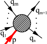
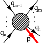
Figure 1: Scattering processes corresponding to cut diagrams in which $n$ internal lines are cut. $m$ runs from $0$ to $n$.

According to the Cutkosky rules generalized at finite temperature Weldon (1983); Kobes and Semenoff (1985, 1986); Jeon (1993); Le Bellac (2000), one can relate $\Im{\rm m}\Sigma_{\rm R}$ to the sum of cut diagrams. The cut diagrams, in which $n$ internal lines are cut, can be interpreted as the scattering processes shown in Fig. 1 where an incoming (outgoing) particle with $p^{\mu}$ disappears (emerges) through the scattering with particles in the heat bath. More precisely, shown in the left diagram of Fig. 1 is the process where a particle with momentum $p$ scatters off $m$ particles with momenta $q_{1},\cdots,q_{m}$ in the heat bath, and turns to $n-m$ particles with momenta $q_{m+1},\cdots,q_{n}$ in the final state. The right diagram shows the reverse process.

Consider the soft limit of our interest $p\to 0$, where the energy-momentum conservation between the initial and final states, $q_{1}+\cdots+q_{m}=q_{m+1}+\cdots+q_{n}$, must be fulfilled. Clearly, the process in which there are no incoming particles from the heat bath (i.e., the initial total energy-momentum is zero) does not contribute to Eq. (4) because the condition for the final total energy-momentum $q_{1}+\cdots+q_{n}=0$ can never be satisfied for massive particles in the heat bath. From this simple observation one concludes that $\Im{\rm m}\Sigma_{\rm R}(p_{0}\to 0,{\boldsymbol{p}}\to 0)=0$ at $T=0$, that is, there is no infrared dissipation in the vacuum. At $T\neq 0$, however, the imaginary part of the self-energy $\Im{\rm m}\Sigma_{\rm R}(p_{0}\to 0,{\boldsymbol{p}}\to 0)$ receives, in general, contributions from the processes where the incoming particle scatters off particles in the heat bath and contributions from their reverse processes.

A more careful inspection reveals that the imaginary part of the self-energy $\Im{\rm m}\Sigma_{\rm R}(p_{0},{\boldsymbol{p}})$ can be written in a rather intuitive form:

$$\Im{\rm m}\Sigma_{\rm R}(p_{0},{\boldsymbol{p}})\sim\sum_{n}\sum_{m=0}^{n}\int dq_{1}\cdots dq_{n}\,\rho^{(m)}(p;q_{1},\cdots,q_{m})\rho^{(n-m)}(q_{m+1},\cdots,q_{n})$$

$$\hskip 85.35826pt\times\Big{\{}{\cal N}[f_{q_{1}},\cdots,f_{q_{n}}]-\bar{\cal N}[f_{q_{1}},\cdots,f_{q_{n}}]\Big{\}}\;,$$ (5)

where $\rho^{(m)}$ and $\rho^{(n-m)}$ are, respectively, spectral functions for incoming and outgoing thermal particles, and ${\cal N}[\{f_{i}\}]$ is the statistical weight of particles participating in this process ($\bar{\cal N}[\{f_{i}\}]$ is for the reverse process). The weight ${\cal N}[\{f_{i}\}]$ will be expressed as a product of thermal distribution functions $f_{p}=({\rm e}^{\beta|p_{0}|}-1)^{-1}$. The spectral functions specify kinematical windows for scattering states. Therefore, the quantity $\Im{\rm m}\Sigma_{\rm R}(p_{0},{\boldsymbol{p}})$ is non-vanishing when the kinematical windows for the incoming and outgoing particles have overlap with each other. This is a very useful point of view when we evaluate $\Im{\rm m}\Sigma_{\rm R}(p_{0},{\boldsymbol{p}})$ in a concrete model. We will indeed see below that $\Im{\rm m}\Sigma_{\rm R}(p_{0},{\boldsymbol{p}})$ in the $O(N)$ scalar model can be written in this form, and we can assess if it is zero or nonzero by checking the kinematical windows.

Note that we will also treat “composite” fields such as $\varphi^{2}$ since the Schwinger-Dyson equation relates two-point functions to higher-point functions, which could have two (or more) fields at the same space-time point. Similar consideration as discussed above should hold for those “composite” fields.

III Relaxation constant at NLO in $1/N$ expansion

In this paper, as a typical example of relativistic quantum field theories, we employ an $O(N)$-symmetric $\varphi^{4}$ model in $(d+1)$-dimensional space-time with the action

$$S[\varphi]=\int dtd^{d}x\left[\frac{1}{2}\partial_{\mu}\varphi_{a}(x)\partial^{\mu}\varphi_{a}(x)-\frac{m_{0}^{2}}{2}\varphi_{a}(x)\varphi_{a}(x)-\frac{\lambda_{0}}{4!N}(\varphi_{a}(x)\varphi_{a}(x))^{2}\right]\,,$$ (6)

where $\varphi_{a}$ ($a=1,\cdots,N$) is an $N$-component real scalar field, $m_{0}^{2}$ and $\lambda_{0}$ are the bare mass and coupling constant, and we assume $d\leq 3$ so that the action is renormalizable. The partition function in the imaginary time formalism is given by

$$Z[J,K] = \int\limits_{\varphi(0,{\boldsymbol{x}})=\varphi(-i\beta,{\boldsymbol{x}})}{\cal D}\varphi{\rm exp}\left[-S[\varphi]+\int dtd^{d}x\,J_{a}(x)\varphi_{a}(x)+\int dtd^{d}xdt^{\prime}d^{d}y\,\varphi_{a}(x)K_{ab}(x,y)\varphi_{b}(y)\right],$$

where $\beta=1/T$, and we have introduced one- and two-point source fields, $J$ and $K$, respectively. From this partition function $Z[J,K]$, one can introduce the 2PI effective action via a double Legendre transform in $J$ and $K$, while the ordinary 1PI effective action is defined as the single Legendre transform in $J$ with $K\equiv 0$. The advantage of the 2PI effective action is that it reorganizes the perturbative expansion series by resuming the higher-order terms self-consistently into the two-point correlation function. Details of the formalism of the 2PI effective action are presented in Ref. Berges (2005).

In the following calculation, we employ the $1/N$ expansion, which is a typical non-perturbative expansion. The LO contribution is the so-called tadpole diagram which only brings in a shift of the mass $m_{0}^{2}\to m^{2}$. Here we restrict ourselves to the symmetric phase: $m^{2}>0$. The scattering processes among the particles appear at the NLO and in higher order diagrams. The NLO diagram for the self-energy that is relevant for the scattering processes is found to be

$$\Sigma^{\rm scatt.}(i\omega_{n},{\boldsymbol{p}}) =$$ (8)

$$= \raisebox{0.0pt}{\includegraphics[width=79.6678pt]{sig1.eps}}+\raisebox{0.0pt}{\includegraphics[width=91.04872pt]{sig2.eps}}+\cdots+\raisebox{0.0pt}{\includegraphics[width=102.43008pt]{sig3.eps}}\ .$$

The straight line and the wiggly line in Eq. (8), respectively, denote the Matsubara Green function of the elementary field $\varphi$, i.e. $G\sim\left<\varphi\varphi\right>$, and that of the the composite field $\varphi^{2}$, i.e. $D\sim\left<\varphi^{2}\varphi^{2}\right>$. The Matsubara Green function $D(i\omega_{n},{\boldsymbol{p}})$ satisfies the following diagrammatic equation in general:

$$D(i\omega_{n},{\boldsymbol{p}})\ =\ \raisebox{-19.91684pt}{\includegraphics[width=119.50148pt]{D-1.eps}}\ .$$ (9)

The blob in Eq. (9) denotes a vertex function $\left<\varphi^{2}\varphi\varphi\right>$. This vertex function has been studied with a self-consistent equation in Refs. Aarts and Martinez R. (2004); Saito et al. (2012). For the purpose of evaluating the self-energy at NLO, however, we only need this vertex function at LO and then the equation reduces to a geometric series of the one-loop bubble diagram $\Pi(i\omega_{n},{\boldsymbol{p}})$ which leads to the second line of Eq. (8):

$$D(i\omega_{n},{\boldsymbol{p}}) = \ \ \raisebox{-8.5359pt}{\includegraphics[width=45.52458pt]{9.eps}}\ \ +\ \ \raisebox{-7.11317pt}{\includegraphics[width=165.02606pt]{10.eps}}$$ (10)

$$= \frac{\Pi(i\omega_{n},{\boldsymbol{p}})}{1+\frac{\lambda}{6}\Pi(i\omega_{n},{\boldsymbol{p}})}\;.$$

At the end of the calculation we perform the analytic continuation from the imaginary to the real energy. Then the imaginary-time correlators are replaced by their retarded counterparts which are explicitly defined as

$$G^{ab}_{\rm R}(p_{0},{\boldsymbol{p}})=G_{\rm R}(p_{0},{\boldsymbol{p}})\delta_{ab} = \int dtd{\boldsymbol{x}}\ {\rm e}^{i(p_{0}t-{\boldsymbol{p}}\cdot{\boldsymbol{x}})}\theta(t)\left<[\varphi_{a}(t,{\boldsymbol{x}}),\varphi_{b}(0,{\boldsymbol{0}})]\right>,$$ (11)

$$D_{\rm R}(p_{0},{\boldsymbol{p}}) = \ \int dtd{\boldsymbol{x}}\ {\rm e}^{i(p_{0}t-{\boldsymbol{p}}\cdot{\boldsymbol{x}})}\theta(t)\left<[\varphi^{2}(t,{\boldsymbol{x}}),\varphi^{2}(0,{\boldsymbol{0}})]\right>.$$ (12)

Here $G_{\rm R}^{ab}=G_{\rm R}\,\delta_{ab}$ in the symmetric phase, and the field indices are suppressed in $\varphi^{2}=\varphi_{a}\varphi_{a}$ and

$$D_{\rm R}(p) = \frac{\Pi_{\rm R}(p)}{1+\frac{\lambda}{6}\Pi_{\rm R}(p)}\;,$$ (13)

where

$$\Pi_{\rm R}(p) = \int\frac{dq_{0}d{\boldsymbol{q}}}{(2\pi)^{d+1}}\ n(q_{0})\ \rho(q)\ [G_{\rm R}(p+q)+G_{\rm A}(q-p)]\,.$$ (14)

By using all the information given above, one can find the explicit form of the imaginary part of the NLO self-energy Eq. (8) (see Appendix A for derivation)

$$\Im{\rm m}\Sigma_{\rm R}(p) = \frac{\lambda}{6N}\frac{\lambda}{6}\int\frac{dq_{0}d{\boldsymbol{q}}}{(2\pi)^{d+1}}\ \rho(q)\ \rho_{D}(p+q)\ [n(q_{0})-n(p_{0}+q_{0})]\,,$$ (15)

where $n(p_{0})=({\rm e}^{\beta p_{0}}-1)^{-1}$, and the spectral functions for two-point correlators are defined as

$$\rho(p_{0},{\boldsymbol{p}})\equiv 2\ \Im{\rm m}[G_{\rm R}(p_{0},{\boldsymbol{p}})]\ ,\qquad\quad\rho_{D}(p_{0},{\boldsymbol{p}})\equiv 2\ \Im{\rm m}[D_{\rm R}(p_{0},{\boldsymbol{p}})]\;,$$ (16)

Especially, in the LO approximation for $D_{R}$,

$$\rho_{D}(p_{0},{\boldsymbol{p}}) =\frac{\ 2\ {\Im}{\rm m}\Pi_{\rm R}(p_{0},{\boldsymbol{p}})}{\left[1+\frac{\lambda}{6}\ {\Re}{\rm e}\Pi_{\rm R}(p)\right]^{2}+\left[\frac{\lambda}{6}\ {\Im}{\rm m}\Pi_{\rm R}(p_{0},{\boldsymbol{p}})\right]^{2}}\;.$$ (17)

Note that the expression Eq. (15) for $\Im{\rm m}\Sigma_{\rm R}$ at NLO is valid both in the 1PI and 2PI formalisms, except that $G$ is the free propagator in the 1PI formalism while it is the full self-consistent propagator in the 2PI formalism. Note also that Eq. (15) has the form as alluded before in Eq. (5). Namely, one can judge the finiteness of the relaxation constant through the inspection of overlapping kinematical windows specified by the spectral functions $\rho$ and $\rho_{D}$.

In the infrared region, $\Im{\rm m}\Sigma_{\rm R}(p)$ can be approximated as

$$\Im{\rm m}\Sigma_{\rm R}(p) = -\frac{\lambda}{6N}\frac{\lambda}{6}\int\frac{dq_{0}d{\boldsymbol{q}}}{(2\pi)^{d+1}}\ \rho(q_{0},{\boldsymbol{q}})\ \rho_{D}(q_{0},{\boldsymbol{q}})\ p_{0}\ n^{\prime}(q_{0})+{\cal O}({\boldsymbol{p}}^{2},\ p_{0}^{2}).$$ (18)

Substituting Eq. (18) into Eq. (4), we find the equation which determines the relaxation constant $\Gamma$. The aim of the present paper is to show that $\Gamma$ is nonzero finite. For notational brevity, we define a constant $\gamma$ by

$$\frac{1}{\gamma}\equiv-\int\frac{dq_{0}d{\boldsymbol{q}}}{(2\pi)^{d+1}}\ \rho(q_{0},{\boldsymbol{q}})\ \rho_{D}(q_{0},{\boldsymbol{q}})\ n^{\prime}(q_{0})\;,$$ (19)

which is proportional to $\Gamma$. In the following subsections, we will examine if $\gamma$ is nonzero finite at the NLO of the $1/N$ expansion in 1PI and 2PI formalisms.

III.1 1PI-NLO evaluation

First, we confirm that a dissipative mode does not emerge in the 1PI two-point function at the NLO. In the perturbative expansion in the 1PI formalism, the propagator $G_{\rm R}$ appearing in the diagrams is the free propagator obtained at LO with the tadpole effect included in the self-energy, whose spectral function is

$$\rho(p_{0},{\boldsymbol{p}})=2\pi\,{\rm sign}(p_{0})\,\delta(p_{0}^{2}-{\boldsymbol{p}}^{2}-m^{2}).$$ (20)

The other function $\rho_{D}(p_{0},{\boldsymbol{p}})$ in Eq. (19) is the spectral function for a “composite” $\varphi^{2}$ field. Because the $\lambda\varphi^{4}$ interaction couples the $\varphi^{2}$ field with two $\varphi$ fields in either way of $\varphi^{2}\varphi\to\varphi$ or $\varphi^{2}\to\varphi\varphi$ (or their reverse processes), the spectral function $\rho_{D}(p_{0},{\boldsymbol{p}})$ is nonzero in two kinematical regions: the space-like region $s=p_{0}^{2}-{\boldsymbol{p}}^{2}<0$ and two-particle continuum region $s>(2m)^{2}$. The supports of the spectral functions $\rho(p_{0},{\boldsymbol{p}})$ and $\rho_{D}(p_{0},{\boldsymbol{p}})$ do not overlap, and therefore the integral (19) for $(1/\gamma)_{\rm 1PI}$ at NLO vanishes. Therefore, we conclude that, in the 1PI-NLO calculation, dissipation is not seen in the infrared limit of the $\varphi$ mode.

One obvious way to proceed is to go beyond the NLO in the 1PI framework. At the NNLO the expression for the relaxation constant becomes more involved than Eq. (19), but it certainly gives a nonzero value because it is known that the spectral functions $\rho$ and $\rho_{D}$ become nonzero except for $p_{0}=0$ on the $p_{0}$-$p$ plane once the so-called sunset diagram is included in the self-energy Jeon (1995); Blaizot and Iancu (2002); Nishikawa et al. (2003). The sunset diagram appears as a sub-diagram in the NNLO-1PI calculation (e.g., see Fig. 2, where the wavy line in red includes a sunset diagram). We will report progress in this approach in a separate paper xxx .

Figure 2: One of the NNLO diagrams in the 1PI calculation. The sub-diagram in red can be interpreted as a dressing of the propagator $G$, which gives nonzero spectral strength except for $p_{0}=0$ on the $p_{0}$-${\boldsymbol{p}}$ plane.

In this paper, we take another direction. While keeping the NLO approximation, we exploit the 2PI effective action formalism, which self-consistently takes into account the processes relevant to dissipation in the self-energy of the two-point function $G$.

III.2 2PI-NLO evaluation

Let us now confirm that the existence of a dissipative mode is accommodated in the 2PI-NLO calculation by showing that Eq. (19) is nonzero finite. As we have already emphasized several times, the 2PI effective action self-consistetnly determines two-point functions (and the condensate $\left<\varphi\right>$ if $O(N)$ symmetry is broken). The self-consistent structure is seen in the expression (15) of $\Im{\rm m}\Sigma_{\rm R}(p_{0},{\boldsymbol{p}})$ at NLO: it is given by the spectral functions $\rho$ and $\rho_{D}$, but they are in turn given as imaginary parts of two-point functions. Therefore, the precise form of $\Im{\rm m}\Sigma_{\rm R}(p_{0},{\boldsymbol{p}})$ is found only after the Schwinger-Dyson-type equation is solved self-consistently. We are going to show, however, from general properties of the spectral functions $\rho$ and $\rho_{D}$ that $\Im{\rm m}\Sigma_{\rm R}(p_{0},{\boldsymbol{p}})$ in 2PI-NLO has a term proportional to $p_{0}$ with a finite coefficient.

Recall that, in the 1PI-NLO calculation, the supports of two spectral functions $\rho$ and $\rho_{D}$ do not have overlap in the $(q_{0},{\boldsymbol{q}})$ space, giving a vanishing result for Eq. (19), but that 1PI-NNLO will give a nonzero finite result thanks to the sunset diagram as included in Fig. 2. The same contribution is included in the 2PI-NLO diagrams (where we use full propagators) and thus Eq. (19) becomes nonzero finite. Because the spectral functions are odd in the frequency $q_{0}$ and $n^{\prime}(x)=n^{\prime}(-x)=-{\rm e}^{x}/({\rm e}^{x}-1)^{2}$, Eq. (19) yields

$$\frac{1}{\gamma} = \frac{\Omega_{d}}{(2\pi)^{d+1}}\int_{0}^{\infty}dq_{0}\int_{0}^{\infty}q^{d-1}dq\ \rho(q_{0},q)\rho_{D}(q_{0},q)\ \frac{{\rm e}^{\beta q_{0}}}{({\rm e}^{\beta q_{0}}-1)^{2}}\,,$$ (21)

where $\Omega_{d}=\frac{2\pi^{d/2}}{\Gamma(d/2)}$ is the surface area of the $d$-dimensional sphere. Since the spectral functions $\rho$ and $\rho_{D}$ are positive semi-definite for $q_{0}>0$ in general, and, as mentioned above, they have nonzero values except for $p_{0}=0$ in the integration domain in the 2PI-NLO calculation Jeon (1995); Blaizot and Iancu (2002); Nishikawa et al. (2003), we conclude at this point that Eq. (21) has a nonzero value, in constrast to the 1PI-NLO result.

In the following, we verify that Eq. (21) for $1/\gamma$, is not diverging, but finite. To this end, we first notice that the spectral functions would not have singularities. For example, the delta-function singularity of $\rho$ coming from the one-particle pole in the vacuum turns into a peak with a finite width due to the interactions in the heat bath. Therefore we can reasonably assume that the integrand does not have any singularity.

Then, what remains to be checked is the behavior of the integrand in the infrared (IR) and ultraviolet (UV) regions. For that purpose, we change the variables from $(q_{0},q)$ to $(Q,\theta)$ defined by $q_{0}=Q\cos\theta,\ q=Q\sin\theta$:

$$\frac{1}{\gamma} = \frac{\Omega_{d}}{(2\pi)^{d+1}}\int_{0}^{\pi/2}d\theta\int_{0}^{\infty}QdQ\ (Q\sin\theta)^{d-1}\ \rho(Q,\theta)\rho_{D}(Q,\theta)\ \frac{{\rm e}^{\beta Q\cos\theta}}{({\rm e}^{\beta Q\cos\theta}-1)^{2}}.$$ (22)

In terms of these new variables, the IR and UV limits correspond to $Q\to 0$ and $Q\to\infty$, respectively, while there is no restriction on the angle $\theta$. Thus, we evaluate the integrand in these limiting regions, and then perform the integration over $\theta$ to check the finiteness of the integral.

Consider the IR region, $\beta Q\ll 1$, where the integrand of Eq. (22) is approximated as

$$Q^{d}\ (\sin\theta)^{d-1}\ \frac{\rho(Q,\theta)}{Q\cos\theta}\ \frac{\rho_{D}(Q,\theta)}{Q\cos\theta}.$$ (23)

In the IR limit $Q\to 0$, spectral functions $\rho$ and $\rho_{D}$ are finite as long as the mass is kept finite, and thus the quantities $\frac{\rho(Q,\theta)}{Q\cos\theta}$ and $\frac{\rho_{D}(Q,\theta)}{Q\cos\theta}$ are finite since $\rho$ and $\rho_{D}$ are proportional to the frequency $q_{0}=Q\cos\theta$, and lastly the $\theta$ integral is also finite (for $d>0$). Hence, we conclude that no divergence appears from the IR region.

Next, we do not expect any divergence either in the UV limit $Q\to\infty$, because physically nonzero $1/\gamma$ should be purely in-medium effect as is seen in the integrand that contains $n^{\prime}(q_{0})$. As long as $\theta\neq\pi/2$, the last factor in the integrand gives an exponential suppression $\sim{\rm e}^{-\beta Q\cos\theta}$ as $Q\to\infty$. The remaining part gives at most positive power of $Q$, as we will see later. Therefore, there is no UV divergence for $\theta\neq\pi/2$.

The only concern is the integrand when the angle $\theta$ is close to $\pi/2$, namely, in a deep space-like region $q_{0}=Q\cos\theta\to 0,\ q=Q\sin\theta\to\infty$. No matter how $Q$ is large, we can take the quantity $\beta Q\cos\theta$ small enough by choosing $\theta$ very close to $\pi/2$. Then, we find a different estimate $\sim 1/(\beta Q\cos\theta)^{2}$ for the last factor in the integrand. Let us define an angle $\alpha$ which satisfies $\beta Q\cos\alpha\ll 1$, or equivalently, ${\pi}/{2}-\alpha\ll\frac{1}{\beta Q}$. We estimate the UV behavior of Eq. (22) by putting $\alpha$ as the lower limit of the integral:

$$\frac{\Omega_{d}}{(2\pi)^{d+1}}\int_{\alpha}^{\pi/2}d\theta\int^{\infty}QdQ\ (Q\sin\theta)^{d-1}\ \rho(Q,\theta)\rho_{D}(Q,\theta)\ \frac{{\rm e}^{\beta Q\cos\theta}}{({\rm e}^{\beta Q\cos\theta}-1)^{2}}$$ (24)

$$\leq\frac{\Omega_{d}}{(2\pi)^{d+1}}\int_{\alpha}^{\pi/2}d\theta\int^{\infty}QdQ\ (Q\sin\theta)^{d-1}\ \rho(Q,\theta)\rho_{D}(Q,\theta)\ \frac{1}{(\beta Q\cos\theta)^{2}}.$$

Since $\rho$ and $\rho_{D}$ are proportional to $q_{0}=Q\cos\theta$ when $\beta q_{0}$ is small enough, the integrand is regular in the limit $\beta Q\cos\theta\to 0$. Let us now introduce two functions as follows:

$$h_{1}(Q)\equiv\lim_{\theta\to\pi/2}\frac{\rho(Q,\theta)}{Q\cos\theta},\qquad\quad h_{2}(Q)\equiv\lim_{\theta\to\pi/2}\frac{\rho_{D}(Q,\theta)}{Q\cos\theta}.$$ (25)

Then, the $\theta$-dependence of the integrand can be neglected, and the r.h.s. of Eq. (24) is evaluated as

$$\sim\frac{\Omega_{d}}{(2\pi)^{d+1}}\ \frac{1}{\beta^{2}}\int^{\infty}\left(\frac{\pi}{2}-\alpha\right)\ QdQ\ Q^{d-1}\ h_{1}(Q)\ h_{2}(Q)\,,$$ (26)

where we have used the approximation $\sin\theta\sim 1$ and $\cos\alpha\sim{\pi}/{2}-\alpha$ valid in the vicinity of $\theta=\pi/2$. Using the condition ${\pi}/{2}-\alpha\ll\frac{1}{\beta Q}$, we can further put an upper limit on the integration shown in Eq. (26):

$$\frac{\Omega_{d}}{(2\pi)^{d+1}}\ \frac{1}{\beta^{2}}\int^{\infty}\left(\frac{\pi}{2}-\alpha\right)\ dQ\ Q^{d}\ h_{1}(Q)\ h_{2}(Q)$$ (27)

$$\ll\frac{\Omega_{d}}{(2\pi)^{d+1}}\ \frac{1}{\beta^{3}}\int^{\infty}dQ\ Q^{d-1}\ h_{1}(Q)\ h_{2}(Q)\,.$$

Now the problem has reduced to checking the UV behavior of the quantity,

$$Q^{d-1}\ h_{1}(Q)\ h_{2}(Q)\,.$$ (28)

If this product decays faster than $1/Q$ as $Q\to\infty$, the integral is UV-finite. In order to know high-momentum behavior of the functions $h_{1}$ and $h_{2}$, a naive dimensional analysis is sufficient.

Since the mass dimensions of $\rho$ and $\rho_{D}$ are $-2$ and $0$, respectively, those of $h_{1}$ and $h_{2}$ in Eq. (25) become $-3$ and $-1$. We define two dimensionless functions $\widetilde{h}_{1}$ and $\widetilde{h}_{2}$ as follows:

$$h_{1}=\frac{1}{Q^{3}}\ \widetilde{h}_{1}\left(\frac{T}{Q},\frac{m}{Q},\frac{\lambda}{Q^{3-d}}\right),\qquad\quad h_{2}=\frac{1}{Q}\ \widetilde{h}_{2}\left(\frac{T}{Q},\frac{m}{Q},\frac{\lambda}{Q^{3-d}}\right)\,,$$ (29)

where we have provided the overall mass-dimensions by $Q$ and explicitly shown the dependence on other dimensionful papameters $T,\ m$ and $\lambda$. If these parameters enter $\widetilde{h}_{1}$ and $\widetilde{h}_{2}$ with positive powers in the deep space-like region, the UV behavior of $h_{1}$ and $h_{2}$ is at most determined by the overall factor as $h_{1}\propto 1/Q^{3}$ and $h_{2}\propto 1/Q$. Below, we give a plausible argument for each parameter to verify that it is indeed the case. We will show the finiteness of the functions $h_{1}$ and $h_{2}$ (or $\widetilde{h}_{1}$ and $\widetilde{h}_{2}$) in the vanishing limit of parameters $T,\ m$, and $\lambda$. If the parameters entered the functions with negative powers, the functions would diverge at this limit.

First of all, consider the $T$ dependence and the limit $T\to 0$ corresponding to the vacuum (in the absence of a medium). In the vacuum, scattering of an incoming particle with the heat bath does not occur, and thus only decay of the incoming particle (and its reverse process) is physically possible. Then, the spectral functions $\rho$ and $\rho_{D}$ describe the decay processes $\varphi\to\varphi\varphi\varphi$ and $\varphi^{2}\to\varphi\varphi$, respectively. Since both have thresholds: $s=q_{0}^{2}-{\boldsymbol{q}}^{2}>(3m)^{2}$ for $\rho$ and $s>(2m)^{2}$ for $\rho_{D}$, one finds $\rho$ and $\rho_{D}$ are zero in the space-like region $s<0$, and do not diverge in the limit $T\to 0$. This means that $\rho$ and $\rho_{D}$, and so $\widetilde{h}_{1}$ and $\widetilde{h}_{2}$, depend on $T$ with positive powers.

Second, consider the $m$ dependence and the $m\to 0$ limit in the space-like region. As long as we stay in a deep space-like region where $|{\boldsymbol{q}}|\gg m$, the $m$ dependent contributions in two-point functions are sub-leading and are given as positive powers of $m/|{\boldsymbol{q}}|$ (this is evident if one considers a free propagator which can be expanded with respect to powers of $m/|{\boldsymbol{q}}|$). Therefore, in the high momentum region, there is no divergence in spectral functions $\rho$ and $\rho_{D}$, and thus in $\widetilde{h}_{1}$ and $\widetilde{h}_{2}$ when we take the limit $m\to 0$.

Third and lastly, consider the $\lambda$ dependence and the limit $\lambda\to 0$, namely the non-interacting system. In this case, $\rho$ is given by the delta-function Eq. (20), and therefore does not diverge in the space-like region. Thus, $\widetilde{h}_{1}$ depends on $\lambda$ with a positive power in the space-like region. The other spectral function $\rho_{D}$ is given by a single bubble diagram (see Eqs. (10), (16)),

$$\rho_{D}(q)=2{\Im}{\rm m}\Pi_{\rm R}(q).$$ (30)

Therefore, both $\rho$ and $\rho_{D}$, and thus $h_{1}$ and $h_{2}$, are finite in the limit $\lambda\to 0$, implying that they are functions of positive powers of $\lambda/Q$. In the free limit $\lambda\to 0$, we can even evaluate the function $h_{2}$ explicitly. Note that in this case ($\lambda=0$) the two-point function is given by a free propagator:

$$G_{\rm R}(q)=\frac{1}{-(q_{0}+i\epsilon)^{2}+{\boldsymbol{q}}^{2}-m^{2}},$$ (31)

where $\epsilon$ is an infinitesimal positive number. After analytic calculation, we obtain

$$h_{2}=\lim_{q_{0}\to 0}\frac{\rho_{D}(q)}{q_{0}}=\frac{1}{4\pi|{\boldsymbol{q}}|}\ \frac{1}{{\rm e}^{\sqrt{{\boldsymbol{q}}^{2}+4m^{2}}/2T}-1}\,.$$ (32)

Therefore, the overall mass-dimension is given by $1/|{\boldsymbol{q}}|\propto Q^{-1}$ which is consistent with the naive dimensional counting as shown in Eq. (29), and $T$ and $m$ dependences appear with positive powers.

Collecting all the results, we conclude that the high-momentum behavior of $h_{1}$ and $h_{2}$ are at most $h_{1}\sim Q^{-3}$ and $h_{2}\sim Q^{-1}$, respectively. Then, the dimension of the integrand in Eq. (27) becomes $Q^{d-5}$ and thus the integral is convergent for $d<4$ which includes the dimensions of our interest, $d\leq 3$.

Hence, in case of the spatial dimension $d\leq 3$, Eq. (22) becomes nonzero and finite constant. Thus, we finally conclude that

$$\left(\frac{1}{\gamma}\right)_{\rm 2PI}\neq 0,\ \infty\,.$$ (33)

This means that a two-point correlation function obtained from the self-consistent equation in 2PI effective action has a dissipative mode in the IR region.

Some comments are in order. First of all, we emphasize that multi-scattering processes in the heat bath are taken into account in the 2PI-NLO but not in the 1PI-NLO calculation. As a result the dissipative mode, which does not exist in the free theory, appears nonperturbatively in the 2PI-NLO calculation. Second, it should be noticed that the dissipative mode emerges irrespective of whether the microscopic field theory is relativistic or nonrelativistic. This fact implies the same scaling behavior of the dissipative mode for the relativistic and nonrelativistic field theory at the critical point. These are in contrast to the propagating modes. The propagating modes exist in the free theory and have different dispersion relations in relativistic and nonrelativistic cases. They get modified by scatterings in the heat bath to acquire damping widths as well as energy shifts. Therefore, the scaling behavior of the propagating modes for the relativistic and nonrelativistic field theories is in general different. Third, we did not attempt to obtain a numerical value of the relaxation constant, although it is in principle possible if one gets the propagators around thermal equilibrium. Namely, if one solves the Kadanoff-Baym equation near the equilibrium, then one can evaluate $1/\gamma$ defined in Eq. (19) with the resultant solutions. We leave this problem for our future work. Rather, in the next section, we discuss an important consequence deduced from the presence of the diffusion term even without knowing its coefficient.

IV Implications for the dynamic exponent $z$

So far, we have considered the case where the effective mass $m^{2}\equiv m_{0}^{2}-\Re{\rm e}\Sigma_{\rm R}(p=0)$ is nonzero. Roughly speaking, the limit $m\to 0$ corresponds to the critical point where the correlation length diverges $\xi\sim 1/m\to\infty$. This divergence also affects the time evolution of a disturbed system towards equilibrium. Off the critical point $m\neq 0$, small disturbances die away exponentially with the relaxation time $\tau$. As the critical point is approached, the relaxation time becomes enormously long, which is called critical slowing down, and we define the dynamic critical exponent $z$ via $\tau\sim\xi^{z}$ Halperin and Hohenberg (1967, 1969); Ferrell et al. (1967a, b); Ferrell et al. (1968). In this section, we first present a consequence on the dynamic critical exponent $z$ from the dissipative mode identified in the previous section, assuming that the relaxation constant $\Gamma$ remains nonzero finite at the critical point. Then we remark possible modification of such a naive assumption.

In order to identify the dynamic critical exponent $z$, we exploit the dynamic scaling relation. We assume that under a scale transformation the two-point function transforms anisotropically with respect to $p_{0}$ and ${\boldsymbol{p}}$:

$$G_{\rm R}(p_{0},{\boldsymbol{p}})=b^{2-\eta}\ G_{\rm R}(b^{z}p_{0},b{\boldsymbol{p}}),$$ (34)

where $b$ is a dimensionless scale factor which is taken bigger than one: $b>1$. The prefactor $b^{2-\eta}$ is fixed by the static part of the two-point function characterized by an exponent $\eta$. Indeed, if one substitutes $b=\Lambda/|{\boldsymbol{p}}|$ into Eq. (34) and sets $p_{0}=0$, one recovers the static scaling for the correlation function $G_{\rm R}^{\rm static}({\boldsymbol{p}})\sim(\Lambda/|{\boldsymbol{p}}|)^{2-\eta}$, where an arbitrary dimensionful parameter $\Lambda$ is introduced to make the combination $\Lambda/|{\boldsymbol{p}}|$ dimensionless. We take $\Lambda$ of the order of the critical temperature $T_{c}$. Next, we will rewrite Eq. (34) into more useful form to evaluate $z$. Since the mass-dimension of $G_{\rm R}$ is $-2$, we can write $G_{\rm R}(p_{0},{\boldsymbol{p}})$ as Hohenberg and Halperin (1977):

$$G_{\rm R}(p_{0},{\boldsymbol{p}})=\left(\frac{\Lambda}{|{\boldsymbol{p}}|}\right)^{2-\eta}\cdot G_{\rm R}\left(\frac{\Lambda^{z}p_{0}}{|{\boldsymbol{p}}|^{z}},\Lambda\right)=\Lambda^{-2}\left(\frac{\Lambda}{|{\boldsymbol{p}}|}\right)^{2-\eta}\cdot\widetilde{G}_{\rm R}\left(\Lambda^{z-1}\frac{p_{0}}{|{\boldsymbol{p}}|^{z}}\right)\,.$$ (35)

Thus, we can extract $z$ from the different scaling properties of $p_{0}$ and ${\boldsymbol{p}}$ in the two-point function.

The self-consistent equation obtained in the 2PI framework is previously utilized to evaluate the static critical exponents $\eta$ Alford et al. (2004) and $\nu$ Saito et al. (2012) (see Ref. Baym and Grinstein (1977); van Hees and Knoll (2002); Alford et al. (2004) for the application of the 2PI framework to 2nd-order phase transitions). While the imaginary part of the self-energy $\Im{\rm m}\Sigma_{\rm R}(p)$ vanishes in the static limit, the momentum dependence of the real part $\Re{\rm e}\Sigma_{\rm R}(p)$ brings in the scaling form of the two-point function:

$$G_{\rm R}^{\rm static}(|{\boldsymbol{p}}|;T_{c})=\Lambda^{-2}\left(\frac{\Lambda}{|{\boldsymbol{p}}|}\right)^{2-\eta}.$$ (36)

Of course, this is the same form as identified in the prefactor in Eq. (34). Since this scaling function is simply obtained from $\Re{\rm e}\Sigma_{\rm R}(p)$, we can substitute it into the two-point function (3) to find the expression at the critical point:

$$G_{\rm R}(p;T_{c})=\frac{1}{-i\Gamma^{-1}p_{0}+{\Lambda^{\eta}}|{\boldsymbol{p}}|^{2-\eta}}=\Lambda^{-2}\left(\frac{\Lambda}{|{\boldsymbol{p}}|}\right)^{2-\eta}\cdot\frac{1}{-i\Gamma^{-1}\Lambda^{-\eta}p_{0}/|{\boldsymbol{p}}|^{2-\eta}+1}\,.$$ (37)

This yields the dynamic critical exponent

$$z=2-\eta\,,$$ (38)

which depends on $N$ and $d$ through $\eta$ Bray (1974); Alford et al. (2004); Vasil’ev (2004).

In order to better understand the result (38), let us carefully see how it appears. For that purpose, it is instructive to go back to the 1PI-NLO calculation which however does not produce a dissipative mode in the IR region. Absence of a dissipative mode in 1PI-NLO is deduced from the IR behavior of $\Im{\rm m}\Sigma_{\rm R}(p)$, namely in the IR region it starts from ${\cal O}(p_{0}^{2},\ {\boldsymbol{p}}^{2})$ instead of ${\cal O}(p_{0})$. Even though we do not have a dissipative mode, we are able to define a “dynamic exponent” from the dispersion relation in the IR region. However, this is an exponent for the “propagating mode” and must be distinguished from the exponent of a dissipative mode which governs very long-time evolution of the system. Indeed, if one considers a propagator in the 1PI-NLO calculation $[G_{\rm R}^{{\rm 1PI-NLO}}(p)]^{-1}\sim{-p_{0}^{2}+{\boldsymbol{p}}^{2}-\Re{\rm e}\Sigma_{\rm R}^{{\rm 1PI-NLO}}(p)-i\Im{\rm m}\Sigma_{\rm R}^{{\rm 1PI-NLO}}(p)}$ with $\Im{\rm m}\Sigma_{\rm R}^{{\rm 1PI-NLO}}(p)={\cal O}(p_{0}^{2},\ {\boldsymbol{p}}^{2})$, one finds dispersions for “propagating modes” $p_{0}\sim\pm|{\boldsymbol{p}}|$ as the leading contribution with small correction from the self-energy of order ${\cal O}(1/N)$. Thus, one will find an exponent $z_{\rm prop.}=1+{\cal O}(1/N)$, where we have introduced $z_{\rm prop.}$ to remind that it is not the exponent for a dissipative mode, but for a propagating mode. If one performs the same analysis in nonrelativistic field theories, one will find $z_{\rm prop.}=2+{\cal O}(1/N)$ again for propagating modes whose leading dispersions are $p_{0}\propto{\boldsymbol{p}}^{2}$. Namely, the leading contribution $z_{0}$ in the exponent $z_{\rm prop.}=z_{0}+{\cal O}(1/N)$ depends on whether the system is relativistic or nonrelativistic, and this is one of the reasons why there was confusion in the literature. Now, coming back to the 2PI-NLO calculation where we do have a dissipative mode, we find that the presence of a dissipative term, $-i\Gamma^{-1}p_{0}$, modifies the dispersion, and the leading contribution to $z$ is given by 2. Higher order correction $-\eta$ to $z=2$ is from $\Re{\rm e}\Sigma_{\rm R}(p)$ and it is of ${\cal O}(1/N)$. Therefore, our result $z=2-\eta$ in Eq. (38) looks similar to the one for nonrelativistic propagating modes $z_{\rm prop.}=2+{\cal O}(1/N)$, but the origin is different.

Let us further proceed one more step. Our result (38) is an immediate consequence of the static scaling behavior under the assumption that the relaxation term $-ip_{0}/\Gamma$ remains non-singular Van Hove (1954a, b). However, the relaxation constant $\Gamma$ may depend on ${\boldsymbol{p}}$ in general. If one assumes $\Gamma\sim\Gamma_{0}\,(|{\boldsymbol{p}}|/\Lambda)^{c^{\prime}}$ with $\Gamma_{0}$ and $c^{\prime}$ being constants in the IR region, then one obtains

$$G_{\rm R}(p_{0},{\boldsymbol{p}})\sim\frac{1}{-i\Gamma_{0}^{-1}(\Lambda/|{\boldsymbol{p}}|)^{c^{\prime}}p_{0}+\Lambda^{\eta}{\boldsymbol{p}}^{2-\eta}}.$$ (39)

and accordingly the exponent $z$ is modified to

$$z=2-\eta+c^{\prime}.$$ (40)

This is also clearly seen in the $t$-dependence of the two point function. Equation (39) leads to $G_{\rm R}(t,{\boldsymbol{p}})\sim\exp\{-t/\tau({\boldsymbol{p}})\}$ where the relaxation time is given by $\tau({\boldsymbol{p}})\sim 1/(\Gamma({\boldsymbol{p}}){\boldsymbol{p}}^{2-\eta})\sim 1/{\boldsymbol{p}}^{2-\eta+c^{\prime}}$. Thus, in the IR region ${\boldsymbol{p}}\to 0$, the relaxation time diverges. We are now working on the evaluation of the numerical value of $c^{\prime}$, and the result will be reported soon elsewhere xxx .

Our result (40) with modified $\Gamma$ is consistent with “model A” in the classification for nonrelativistic systems based on the mode-coupling theory Hohenberg and Halperin (1977). Model A contains only (multi-component) non-conserved fields without conserved fields, and the dynamic critical exponent is given by $z=2+c\eta$, where $c$ is a numerical constant of order one Hohenberg and Halperin (1977); Halperin et al. (1972). It seems apparently to be the case since we are only looking at the fundamental field $\varphi$. But it is actually nontrivial because in the 2PI framework the energy-momentum tensor is conserved and the coupling between the non-conserved fields $\varphi$ and conserved fields is relevant to the dynamic universality classification. However, without knowing the explicit numerical value for $c^{\prime}$, it is difficult at present to judge to which model our result is classified.

There is an explicit numerical simulation for a particular case with $N=1$ and $d=2$ Berges et al. (2010). From numerical evaluation of the dynamic critical exponent $z\sim\frac{2-\eta}{0.87}$, it is claimed that it belongs to the dynamic universality class, model C. However, since we have used the $1/N$ expansion, which is not valid for $N=1$, we cannot directly compare ours to the numerical simulation result, which is intriguing , though.

V Summary

Long-time behavior of a system recovering equilibrium should be characterized by a dissipative hydrodynamic mode. Because of the non-linear mixing among the modes, we expect that even the two-point function $G$ of the order parameter field $\varphi$ carries the information of this long-time dissipation.

We have shown, however, that the NLO calculation of $G$ in the 1PI $1/N$ expansion only gives real and imaginary corrections to the propagating mode of $\delta\varphi$, but it does not generate the dissipative mode in $G$, especially that the imaginary part of the self-energy, ${\Im}{\rm m}\Sigma_{\rm R}(p_{0},{\boldsymbol{p}})/p_{0}$, vanishes in the IR limit, $p_{0},{\boldsymbol{p}}\to 0$. At the critical point, then we find that the mode spectrum scales as $p_{0}\propto p^{z_{\rm prop.}}$ with $z_{\rm prop.}=z_{0}+{\cal O}(1/N)$, where $z_{0}=1$ and 2 for relativistic and nonrelativistic cases, respectively. Since there is no dissipative mode in the IR limit, this exponent is just associated with the propagating mode, whose dispersion depends on whether the system is relativistic or nonrelativistic.

In the 2PI framework, on the other hand, we resumed the multiple scattering effects in the self-consistent propagator $G$ although working at NLO in $1/N$ expansion. Once the self-consistency is imposed on $G$, the spectral function $\rho(p_{0},{\boldsymbol{p}})$ will become nonzero except for $p_{0}=0$ even at the NLO in the $1/N$ expansion. (Recall the sunset diagram for example which is included at this order.) Then we have argued that the dissipative mode inevitably emerges as an IR pole of the propagator $G$ by showing that the imaginary part of the self-energy ${\Im}{\rm m}\Sigma_{\rm R}(p_{0},{\boldsymbol{p}})/p_{0}$ is generally nonzero finite in the IR limit.

At the critical point, this dissipative mode implies that we will have $z\sim 2-\eta$ even in relativistic scalar theories, which is in contrast to the 1PI-NLO result. For more precise evaluation of the exponent $z$, one may need to compute the transport coefficient utilizing the 4PI framework. We leave this as our future work. Furthermore, it is not clear whether the dissipative mode we found is the same as the dissipation of the hydrodynamic mode such as heat. To this end, we apparently need more detailed and systematic evaluation of the coupled two-point functions of $\varphi$ and the energy-momentum densities, etc.

Appendix A Derivation of Eq. (15)

In this Appendix, we derive Eq. (15) in spatial $d$-dimensions using imaginary time formalism. As we have graphically shown in Eq. (8), the (scattering part of the) self-energy at NLO is explicitly written as

$$\Sigma(i\omega_{n},{\boldsymbol{p}})=\frac{\lambda}{3N}\ \frac{\lambda}{6}\ T\sum_{m}\int\frac{d{\boldsymbol{q}}}{(2\pi)^{d}}\ G(i\omega_{m},{\boldsymbol{q}})\ D(i\omega_{n+m},{\boldsymbol{p}}+{\boldsymbol{q}})\,,$$ (41)

where $i\omega_{n}$ is the Matsubara frequency, $i\omega_{n}=2\pi in/\beta\ (n\in\mathbb{Z})$. In the 1PI formalism, $G$ and $D$ are free correlation functions, and summation over the Matsubara frequency is easily transformed into a contour integral on a complex plane of an analytically continued variable $\zeta$. On the other hand, in the 2PI formalism, $G(i\omega_{n},{\boldsymbol{q}})$ and $D(i\omega_{n},{\boldsymbol{q}})$ are full correlation functions and, when analytically continued, both $G(\zeta,{\boldsymbol{q}})$ and $D(\zeta,{\boldsymbol{q}})$ have cuts along the real axis $\Im{\rm m}\,\zeta=0$ except for the origin $\zeta=0$. Namely, $G(\zeta,{\boldsymbol{q}})$ and $D(\zeta,{\boldsymbol{q}})$ have discontinuities along the real axis, but one can define $G(0,{\boldsymbol{q}})$ and $D(0,{\boldsymbol{q}})$ without ambiguity. Thus, we have to be careful when we transform the Matsubara summation into a contour integral over the complex variable $\zeta$ Holstein (1964); Valle Basagoiti (2002). This was done in Ref. Aarts and Martinez R. (2004) when the spatial dimension $d$ is three. Here, we will follow Ref. Aarts and Martinez R. (2004), but work in $d$ dimensions.

In the complex plane of $\zeta$, one can recover the Matsubara summation by picking up all the residues of the function, $n(\zeta)=({\rm e}^{\beta\zeta}-1)^{-1}$. Therefore, Eq. (41) becomes

$$\Sigma(i\omega_{n},{\boldsymbol{p}})=\frac{\lambda}{3N}\ \frac{\lambda}{6}\ \int_{\cal C}\frac{d\zeta}{2\pi i}\int\frac{d{\boldsymbol{q}}}{(2\pi)^{d}}\ n(\zeta)\ G(\zeta,{\boldsymbol{q}})\ D(i\omega_{n}+\zeta,{\boldsymbol{p}}+{\boldsymbol{q}}),$$ (42)

where the integral-contour ${\cal C}$ is a collection of circles going around counterclockwise each pole of $n(\zeta)$: $\zeta=2\pi im/\beta\ (m\in\mathbb{Z})$. We have to be careful when we pick up the poles at $\zeta=0$ and $\zeta=-i\omega_{n}$ because there are cuts originating from the same points. The easiest way to avoid this is to infinitesimally shift the poles so that one can safely pick up the residues. This simple prescription indeed works and the result does not depend on the way how to shift the poles.

Then, we modify the contour ${\cal C}$ (collection of small circles around the poles of $n(\zeta)$) paying attention to the presence of cuts along $\zeta=0$ and $\zeta=-i\omega_{n}$, and obtain a new contour ${\cal C^{\prime}}$ as shown in Fig. 3.

Figure 3: The complex plane of $\zeta$. Dotted lines along ${\Im}{\rm m}\ \zeta=0$ and ${\Im}{\rm m}\ \zeta=-\omega_{n}$ represent cuts of $G(\zeta)$ and $D(i\omega_{n}+\zeta)$, respectively. The crosses denote poles of $n(\zeta)$, all of which are on the imaginary axis. The contour ${\cal C}$ can be modified to three closed paths ${\cal C}^{\prime}$ (solid lines).

In this integral, contributions from infinite distances become zero. Therefore, we pick up the integrals along two discontinuities. Namely, we consider four paths: from $\zeta=-\infty\pm i\epsilon$ to $\zeta=+\infty\pm i\epsilon$, and from $\zeta=-\infty-i\omega_{n}\pm i\epsilon$ to $\zeta=+\infty-i\omega_{n}\pm i\epsilon$ ($\epsilon$ is an infinitesimal positive number). Thus, we find that Eq. (42) becomes

$$\Sigma(i\omega_{n},{\boldsymbol{p}}) = \frac{\lambda}{3N}\ \frac{\lambda}{6}\ \int_{-\infty}^{\infty}\frac{dq_{0}}{2\pi i}\int\frac{d{\boldsymbol{q}}}{(2\pi)^{d}}\ n(q_{0})$$ (43)

$$\times\left\{[G(q_{0}+i\epsilon,{\boldsymbol{q}})-G(q_{0}-i\epsilon,{\boldsymbol{q}})]\ D(i\omega_{n}+q_{0},{\boldsymbol{p}}+{\boldsymbol{q}})\right.$$

$$\quad\left.+G(q_{0}-i\omega_{n},{\boldsymbol{q}})\ [D(q_{0}+i\epsilon,{\boldsymbol{p}}+{\boldsymbol{q}})-D(q_{0}-i\epsilon,{\boldsymbol{p}}+{\boldsymbol{q}})]\right\}.$$

In order to obtain the retarded self-energy, we perform analytic continuation $i\omega_{n}\to p_{0}+i\epsilon$.

$$\Sigma_{\rm R}(p_{0},{\boldsymbol{p}}) = \frac{\lambda}{3N}\ \frac{\lambda}{6}\ \int\frac{dq_{0}d{\boldsymbol{q}}}{(2\pi)^{d+1}}\ n(q_{0})$$ (44)

$$\times\left\{\rho(q_{0},{\boldsymbol{q}})\ D_{\rm R}(p_{0}+q_{0},{\boldsymbol{p}}+{\boldsymbol{q}})+G_{\rm A}(q_{0}-p_{0},{\boldsymbol{q}})\ \rho_{D}(q_{0},{\boldsymbol{p}}+{\boldsymbol{q}})\right\},$$

where we have used the following properties

$$\rho(q_{0},{\boldsymbol{q}})=-i\ [G_{\rm R}(q_{0},{\boldsymbol{q}})-G_{\rm A}(q_{0},{\boldsymbol{q}})],\qquad\ \rho_{D}(q_{0},{\boldsymbol{q}})=-i\ [D_{\rm R}(q_{0},{\boldsymbol{q}})-D_{\rm A}(q_{0},{\boldsymbol{q}})]\ .$$ (45)

Now, we take the imaginary part of Eq. (44). Since the spectral functions are imaginary parts of correlation functions,

$$\rho(p)=2\ {\Im}{\rm m}\ G_{\rm R}(p)=-2\ {\Im}{\rm m}\ G_{\rm A}(p)\,,\ \qquad\rho_{D}(p)=2\ {\Im}{\rm m}\ D_{\rm R}(p)=-2\ {\Im}{\rm m}\ D_{\rm A}(p)\ ,$$ (46)

we finally obtain Eq. (15):

$$\Im{\rm m}\Sigma_{\rm R}(p_{0},{\boldsymbol{p}}) = \frac{\lambda}{6N}\ \frac{\lambda}{6}\ \int\frac{dq_{0}d{\boldsymbol{q}}}{(2\pi)^{d+1}}\ n(q_{0})$$ (47)

$$\times\left\{\rho(q_{0},{\boldsymbol{q}})\ \rho_{D}(p_{0}+q_{0},{\boldsymbol{p}}+{\boldsymbol{q}})-\rho(q_{0}-p_{0},{\boldsymbol{q}})\ \rho_{D}(q_{0},{\boldsymbol{p}}+{\boldsymbol{q}})\right\}$$

$$= \frac{\lambda}{6N}\ \frac{\lambda}{6}\ \int\frac{dq_{0}d{\boldsymbol{q}}}{(2\pi)^{d+1}}\ \rho(q)\ \rho_{D}(p+q)\ [n(q_{0})-n(p_{0}+q_{0})].$$

In the second line of Eq. (47), we have changed the integration variables of the second term as $q_{0}\to q_{0}+p_{0}$ and ${\boldsymbol{q}}\to{\boldsymbol{p}}+{\boldsymbol{q}}$.

References

- Kadanoff and Martin (1963) L. P. Kadanoff and P. C. Martin, Ann. Phys. 24, 419 (1963).
- Halperin and Hohenberg (1967) B. I. Halperin and P. C. Hohenberg, Phys. Rev. Lett. 19, 700 (1967).
- Halperin and Hohenberg (1969) B. I. Halperin and P. C. Hohenberg, Phys. Rev. 177, 952 (1969).
- Kawasaki (1970) K. Kawasaki, Ann. Phys. 61, 1 (1970).
- Hohenberg and Halperin (1977) P. C. Hohenberg and B. I. Halperin, Rev. Mod. Phys. 49, 435 (1977).
- Luttinger and Ward (1960) J. M. Luttinger and J. C. Ward, Phys. Rev. 118, 1417 (1960).
- Cornwall et al. (1974) J. M. Cornwall, R. Jackiw, and E. Tomboulis, Phys. Rev. D10, 2428 (1974).
- Berges (2005) J. Berges, AIP Conf. Proc. 739, 3 (2005), eprint hep-ph/0409233.
- Baym and Kadanoff (1961) G. Baym and L. P. Kadanoff, Phys. Rev. 124, 287 (1961).
- Baym (1962) G. Baym, Phys. Rev. 127, 1391 (1962).
- Kadanoff and Baym (1962) L. P. Kadanoff and G. Baym, Quantum statistical mechanics: Green’s function methods in equilibrium and nonequilibrium problems (Benjamin, 1962).
- Halperin et al. (1972) B. I. Halperin, P. C. Hohenberg, and S.-k. Ma, Phys. Rev. Lett. 29, 1548 (1972).
- Halperin et al. (1974b) B. I. Halperin, P. C. Hohenberg, and E. D. Siggia, Phys. Rev. Lett. 32, 1289 (1974b).
- Halperin et al. (1974a) B. I. Halperin, P. C. Hohenberg, and S.-k. Ma, Phys. Rev. B 10, 139 (1974a).
- Halperin et al. (1976) B. I. Halperin, P. C. Hohenberg, and S.-k. Ma, Phys. Rev. B 13, 4119 (1976).
- Rajagopal and Wilczek (1993) K. Rajagopal and F. Wilczek, Nucl. Phys. B 399, 395 (1993), eprint hep-ph/9210253.
- Nakano et al. (2012) E. Nakano, V. Skokov, and B. Friman, Phys. Rev. D 85, 096007 (2012).
- Ohnishi et al. (2005) K. Ohnishi, K. Fukushima, and K. Ohta, Nucl. Phys. A 748, 260 (2005), eprint nucl-th/0409046.
- Abe (1974) R. Abe, Prog. Theor. Phys. 52, 1135 (1974).
- Abe and Hikami (1974) R. Abe and S. Hikami, Prog. Theor. Phys. 52, 1463 (1974).
- Boyanovsky et al. (2001) D. Boyanovsky, H. J. de Vega, and M. Simionato, Phys. Rev. D 63, 045007 (2001).
- Boyanovsky and de Vega (2003) D. Boyanovsky and H. J. de Vega, Ann. Phys. 307, 335 (2003), eprint hep-ph/0302055.
- Berges et al. (2010) J. Berges, S. Schlichting, and D. Sexty, Nucl. Phys. B 832, 228 (2010), eprint 0912.3135.
- Kolb and Heinz (2004) P. F. Kolb and U. Heinz, in Quark-Gluon Plasma (2004), vol. 1, p. 634.
- Hirano et al. (2010) T. Hirano, N. van der Kolk, and A. Bilandzic, in The Physics of the Quark-Gluon Plasma (Springer, 2010), pp. 139–178.
- Hirano (2011) T. Hirano, Act. Phys. Pol. B 42, 2811 (2011).
- Stringari (1996) S. Stringari, Phys. Rev. Lett. 77, 2360 (1996).
- Takiwaki et al. (2012) T. Takiwaki, K. Kotake, and Y. Suwa, ApJ 749, 98 (2012) and references therein.
- Weinberg (1972) S. Weinberg, Gravitation and cosmology: principles and applications of the general theory of relativity, vol. 1 (Wiley New York, 1972).
- Odyniec (2010) G. Odyniec, J. Phys. G: Nucl. Part. Phys. 37, 094028 (2010).
- Mohanty et al. (2011) B. Mohanty et al., J. Phys. G: Nucl. Part. Phys. 38, 124023 (2011).
- Fujii (2003) H. Fujii, Phys. Rev. D 67, 094018 (2003).
- Fujii and Ohtani (2004) H. Fujii and M. Ohtani, Phys. Rev. D 70, 014016 (2004).
- Son and Stephanov (2004) D. T. Son and M. A. Stephanov, Phys. Rev. D 70, 056001 (2004).
- Berges et al. (2009) J. Berges, S. Scheffler, and D. Sexty, Phys. Lett. B 681, 362 (2009).
- Dusling et al. (2012) K. Dusling et al., Phys. Rev. D 86, 085040 (2012).
- Berges et al. (2013) J. Berges, K. Boguslavski, S. Schlichting, and R. Venugopalan, arXiv:1303.5650 (2013).
- Epelbaum and Gelis (2013) T. Epelbaum and F. Gelis, arXiv preprint arXiv:1307.2214 (2013).
- Gasenzer (2009) T. Gasenzer, EPJST 168, 89 (2009).
- Kubo (1957) R. Kubo, J. Phys. Soc. Jpn. 12, 570 (1957).
- Le Bellac (2000) M. Le Bellac, Thermal field theory (Cambridge University Press, 2000).
- Forster (1975) D. Forster, Hydrodynamic fluctuations, broken symmetry, and correlation functions (WA Benjamin, Inc., Reading, MA, 1975).
- Weldon (1983) H. A. Weldon, Phys. Rev. D 28, 2007 (1983).
- Kobes and Semenoff (1985) R. L. Kobes and G. W. Semenoff, Nuclear Physics B 260, 714 (1985).
- Kobes and Semenoff (1986) R. L. Kobes and G. W. Semenoff, Nuclear Physics B 272, 329 (1986).
- Jeon (1993) S. Jeon, Phys. Rev. D 47, 4586 (1993).
- Aarts et al. (2002) G. Aarts et al., Phys. Rev. D 66, 045008 (2002).
- Aarts and Martinez R. (2004) G. Aarts and J. M. Martinez R., JHEP 02, 061 (2004), eprint hep-ph/0402192.
- Saito et al. (2012) Y. Saito, H. Fujii, K. Itakura, and O. Morimatsu, Phys. Rev. D 85, 065019 (2012).
- Jeon (1995) S. Jeon, Phys. Rev. D 52, 3591 (1995).
- Blaizot and Iancu (2002) J.-P. Blaizot and E. Iancu, Phys. Rep. 359, 355 (2002).
- Nishikawa et al. (2003) T. Nishikawa, O. Morimatsu, and Y. Hidaka, Phys. Rev. D 68, 076002 (2003).
- (53) Y. Saito, H. Fujii, K. Itakura, and O. Morimatsu, in preparation.
- Ferrell et al. (1967a) R. A. Ferrell et al., Phys. Rev. Lett. 18, 891 (1967a).
- Ferrell et al. (1967b) R. A. Ferrell et al., Phys. Lett. A 24, 493 (1967b).
- Ferrell et al. (1968) R. A. Ferrell et al., Ann. Phys. 47, 565 (1968).
- Alford et al. (2004) M. Alford, J. Berges, and J. M. Cheyne, Phys. Rev. D 70, 125002 (2004), eprint hep-ph/0404059.
- Baym and Grinstein (1977) G. Baym and G. Grinstein, Phys. Rev. D 15, 2897 (1977).
- van Hees and Knoll (2002) H. van Hees and J. Knoll, Phys. Rev. D66, 025028 (2002), eprint hep-ph/0203008.
- Bray (1974) A. J. Bray, Phys. Rev. Lett. 32, 1413 (1974).
- Vasil’ev (2004) A. N. Vasil’ev, The Field Theoretic Renormalization Group in Critical Behavior Theory and Stochastic Dynamics (CRC press, 2004).
- Van Hove (1954a) L. Van Hove, Phys. Rev. 95, 249 (1954a).
- Van Hove (1954b) L. Van Hove, Phys. Rev. 95, 1374 (1954b).
- Holstein (1964) T. Holstein, Ann. Phys. 29, 410 (1964).
- Valle Basagoiti (2002) M. A. Valle Basagoiti, Phys. Rev. D 66, 045005 (2002).
- Baym and Mermin (1961) G. Baym and N. D. Mermin, J. Math. Phys. 2, 232 (1961).