Cooling of a Nanomechanical Resonator in Presence of a Single Diatomic Molecule

Abstract

We propose a theoretical scheme for coupling a nanomechanical resonator to a single diatomic molecule via microwave cavity mode of a driven $LC$ resonator. We describe the diatomic molecule by a Morse potential and find the corresponding equations of motion of the hybrid system by using Fokker-Planck formalism. Analytical expressions for the effective frequency and the effective damping of the nanomechanical resonator are obtained. We analyze the ground state cooling of the nanomechanical resonator in presence of the diatomic molecule. The results confirm that presence of the molecule improves the cooling process of the mechanical resonator. Finally, the effect of molecule’s parameters on the cooling mechanism is studied.

Keywords: Quantum ground state cooling, Nanomechanical resonator, Superconducting circuit.

I Introduction

In optomechanical cavity, radiation pressure acts on an oscillating mirror which induces an interaction between the mechanical system and the optical field. The coupling of mechanical and optical degrees of freedom via radiation pressure has been employed for a wide range of applications, such as the cavity cooling of microlevers and nanomechanical resonators to their quantum mechanical ground states Aspelmeyer et al. (2014); Chen (2013); Cleland (2003); Kleckner and Bouwmeester (2006); Poggio et al. (2007); Teufel et al. (2008); Arcizet et al. (2006); Teufel et al. (2011a).

Activity in this field started with experimental observations of optomechanical cooling first using feedback Cohadon et al. (1999), and later using an intrinsic effect Gigan et al. (2006). Aside from optomechanical cooling, electronic cooling was also studied. For instance, schemes have been proposed to replace the optical cavity by radio frequency circuits Brown et al. (2007) or one-dimensional transmission line resonators Xue et al. (2007); Zhang et al. (2009).

Very recently, various schemes have been also proposed in order to couple mechanical resonator to other systems Xiang et al. (2013) including single atoms Hammerer et al. (2009); Wallquist et al. (2010); Chang et al. (2009); Breyer and Bienert (2012); Barzanjeh et al. (2011), atomic ensembles Ian et al. (2008); Schleier-Smith et al. (2011); Genes et al. (2008a), ions Tian and Zoller (2004), molecules Bhattacharya et al. (2010); Singh et al. (2008), and electrons Ciaramicoli et al. (2007). In this direction, as is shown in Ref. Ian et al. (2008), the presence of an atomic ensemble effectively enhances the optomechanical coupling rate. However, a theoretical description of the motion of mechanical resonator based on the capacitive coupling of the resonator with a superconducting coplanar waveguide, was discussed in Ref. Vitali et al. (2007), which focused on studying the entanglement between mechanical resonator and transmission line resonator without considering the cooling of mechanical resonators. Since the quantized electric field of a resonator circuit can be easily coupled to ions Kielpinski et al. (2012) and atoms  Daniilidis and Häffner (2013), then the direct coupling between the electrical circuits and mechanical resonator also utilizes a new way for coupling mechanical resonators either to two-level systems or ions Xiang et al. (2013). It also paves the way for coupling the mechanical resonators to the dipole moment of the diatomic molecules. The diatomic molecules usually can be described by a nonlinear Morse potential. The interaction between a weakly nonlinear Morse oscillator to quantized intracavity field was also studied in Refs. Gangopadhyay and Ray (1990, 1991). The authors used the Jaynes-Cummings like interaction between molecule and electric field in which the dipole of the molecule interacts with electric field of the cavity mode.

Motivated by the aforementioned studies, the basic study here is a Morse oscillator, the simple diatomic molecular system with non-equidistant multi-level states, coupled to a nanomechanical resonator via a microwave cavity mode of a driven superconducting LC resonator. Both the dynamics of the nanomechanical oscillator and the properties of microwave field are modified through this interaction. The purpose of this paper is to investigate the effect of presence of the diatomic molecule on the cooling of the nanomechanical resonator. The Morse oscillator is assumed to be weakly non-linear, and attains an equilibrium with the driving field through the effect of radiation damping only. We omit all other relaxation processes and neglect the wave mixing effects from the present analysis. We derive an exact second-order Fokker-Planck equation for the hybrid system. The Fokker-Planck equation can be converted into an equivalent set of first-order stochastic differential equations, which can be used for studying the cooling of the mechanical resonator.

The paper is structured as follows: In Sec. II, first we present a hybrid system composed of a microwave cavity mode, a nanomechanical resonator, and a diatomic molecule then the Hamiltonian of the hybrid configuration is found. In Sec. III, the stochastic equations corresponding to the Fokker-Planck equation is obtained by Itô’s rule and the dynamics of the systems is discussed. In Sec. IV, we investigate the effective frequency and the effective damping parameter of the nanomechanical oscillator. In Sec. V, the ground state cooling of the nanomechanical resonator is discussed. Finally, a summary and concluding remarks are given in Sec. VI.

II SYSTEM MODEL AND HAMILTONIAN

In this section, first we shortly discuss about the Hamiltonian of a diatomic molecule, then we find the Hamiltonian of a hybrid system in which a nanomechanical resonator couples to a diatomic molecule via microwave cavity mode.

II.1 Morse potential

It is known that the interaction between atoms in a diatomic molecule can be described by anharmonic Morse potential Dong et al. (2003); Angelova and Hussin (2008). The Morse potential can be expressed as Dong et al. (2003)

$$V(r)=D_{e}(1-e^{-a(r-r_{e})})^{2},$$ (1)

where $r$ is the inter-nuclear distance between the atoms, $r_{e}$ is the equilibrium bond distance, $D_{e}$ is the well depth (defined relative to the dissociated atoms), and $a=\omega_{e}\sqrt{\mu/2D_{e}}$ is related with the range of the potential which identifies by reduced mass $\mu$ and fundamental vibrational frequency $\omega_{e}$. The Schrödinger equation for the Morse potential is exactly solvable, giving the vibrational eigenvalues

$$E_{\nu}=\omega_{e}(\nu+1/2)-\frac{\omega_{e}^{2}}{4D_{e}}(\nu+1/2)^{2},$$ (2)

where $\nu=0,1,2,...,\nu_{max}$. Unlike the harmonic oscillator, the Morse potential has a finite number of bound vibrational levels, with $\nu_{max}\simeq 2D_{e}/\omega_{e}$.

Since the system’s dynamics does not change under a constant shift in potential energy then the equation for Morse potential can be rewritten by adding or subtracting a constant value

$$V(r)-D_{e}=D_{e}(e^{-2a(r-r_{e})}-e^{-a(r-r_{e})}).$$ (3)

The Eq. (3) approaches zero at infinite $r$ and equals $-D_{e}$ at its minimum. This shows that the Morse potential is the combination of a short-range repulsion and a longer-range attractive tail. The Hamiltonian of a diatomic molecule can be obtained by adding the kinetic term to potential in Eq. (3). In addition, Eq. (3) plus kinetic energy can be rewritten in the term of the ladder operators $\hat{S}_{\pm}$ and the operator $\hat{S}_{0}$ Dong et al. (2003)

$$\hat{H}_{p} = \hbar\omega_{p}(\hat{S}_{-}\hat{S}_{+}+\hat{S}_{0}),$$ (4)

where the operators $\hat{S}_{\pm}$ and $\hat{S}_{0}$ satisfy the following commutation relations

$$[\hat{S}_{+},\hat{S}_{-}]=2\hat{S}_{0},[\hat{S}_{0},\hat{S}_{\pm}]=\pm\hat{S}_{\pm},$$ (5)

and we have defined the vibrational frequency $\omega_{p}=\frac{\hbar a^{2}}{2\mu}$ which gets values from GHz (for $K_{2}$ molecule) to THz (for $H_{2}$ molecule) Noggle (1996).

Figure 1: (Color online) The coupling between a nanomechanical resonator and a single diatomic molecule via microwave cavity field. A single diatomic molecule, described by a Morse potential with transition frequency $\omega_{p}$, is confined within a microwave cavity in the form of $LC$ circuit. A nanomechanical resonator is also coupled to the central conductor of the microwave cavity via a capacitance $C_{0}(x)$.

II.2 Hamiltonian of the Hybrid system

Now, we are in a position to introduce the hybrid system sketched in Fig. 1. A single diatomic molecule, described by a Morse potential with transition frequency $\omega_{p}$, is confined within a microwave cavity in the form of $LC$ circuit. A nanomechanical resonator is also coupled to the central conductor of the microwave cavity via a capacitance $C_{0}(\hat{x})=C_{0}(1-\hat{x}(t)/d)$. The microwave cavity can be modeled as a single-mode $LC$ resonator with frequency $\omega_{f}=1/\sqrt{LC_{0}}$, where $C_{0}$ and $L$ are the overall capacitance and inductance, respectively. The nanomechanical resonator is modeled as a harmonic oscillator with frequency $\omega_{m}$ and effective mass $m$. The cavity is driven by an external microwave field at frequency $\omega_{0}$, where the coherent driving of cavity is given by the electric potential $E_{d}(t)=-i\sqrt{2\hbar\omega_{f}L}\epsilon_{0}(e^{i\omega_{0}t}-e^{-i\omega_{0}t})$. Therefore, the Hamiltonian of the hybrid system is described by Vitali et al. (2007)

$$\hat{H}=\frac{\hat{p}_{x}^{2}}{2m}+\frac{m\omega_{m}^{2}\hat{x}^{2}}{2}+\frac{\hat{\Phi}^{2}}{2L}+\frac{\hat{Q}^{2}}{2C_{0}(\hat{x})}+\hbar\omega_{p}(\hat{S}_{-}\hat{S}_{+}+\hat{S}_{0})-E_{d}(t)\hat{Q}+\hat{U}_{int}.$$ (6)

where $\hat{x}$ and $\hat{p}_{x}$ are the canonical position and momentum of the nanomechanical resonator, $\hat{\Phi}$ and $\hat{Q}$ denote the canonical coordinates for the microwave cavity with inductance $L$ and capacitance $C_{0}$, and $\hat{U}_{int}$ is the interaction potential of the molecule and the microwave cavity mode. By expanding the capacitive energy around the equilibrium position of the resonator at $d$ as a Taylor series and by using the annihilation (creation) operator $\hat{a}$ $(\hat{a}^{\dagger})$ of the microwave field $([\hat{a},\hat{a}^{\dagger}]=1)$, the Hamiltonian (6) can be rewritten as

$$\hat{H}=\hbar\omega_{f}\hat{a}^{\dagger}\hat{a}+\frac{\hbar\omega_{m}}{2}(\hat{p}^{2}+\hat{q}^{2})+\hbar\omega_{p}(\hat{S}_{-}\hat{S}_{+}+\hat{S}_{0})+\hat{U}_{int}+\frac{1}{2}\hbar G_{0}\hat{q}(\hat{a}+\hat{a}^{\dagger})^{2}+i\hbar\epsilon_{0}(e^{-i\omega_{0}t}-e^{i\omega_{0}t})(\hat{a}+\hat{a}^{\dagger}),$$ (7)

where

$$\hat{a} = \sqrt{\frac{\omega_{f}L}{2\hbar}}\hat{Q}+\frac{i}{\sqrt{2\hbar\omega_{f}L}}\hat{\Phi},$$ (8)

$$\hat{a}^{\dagger} = \sqrt{\frac{\omega_{f}L}{2\hbar}}\hat{Q}-\frac{i}{\sqrt{2\hbar\omega_{f}L}}\hat{\Phi},$$

and

$$G_{0} = \omega_{f}(\frac{1}{2d}\sqrt{\frac{\hbar}{m\omega_{m}}}),$$ (9)

with $\hat{q}=\sqrt{m\omega_{m}/\hbar}\hat{x}$ and $\hat{p}=\hat{p}_{x}/\sqrt{\hbar m\omega_{m}}$.

The molecule’s dipole can interact with the electric field of the capacitor in the microwave cavity. The interaction of a radiation field $|\hat{\vec{E}}|=\hat{E}_{x}\simeq\hat{Q}/(C_{0}d)$ with a dipole of the diatomic molecule can be described by the following Hamiltonian in the dipole approximation Kielpinski et al. (2012); Daniilidis and Häffner (2013)

$$\hat{U}_{int}=e\vec{r}\cdot(E\textbf{x})=\frac{eV_{d}}{d}(\vec{r}\cdot\textbf{x})\simeq\frac{\hat{Q}}{dC_{0}}\Big{[}\sum_{i,j=1,2}\vec{\wp}_{ij}\hat{S}_{i,j}\Big{]}\cdot\textbf{x},$$ (10)

where $V_{d}$ gives the voltage between the plates of capacitance, x is the unit vector in the direction of $x$ axis, and $\vec{\wp}_{ij}=e\langle i|\vec{r}|j\rangle$ is the electric-dipole transition matrix element of the diatomic molecule. Note that, we approximately ignored the direct interaction of the molecule to the motional degree of freedom of the nanomechanical resonator due to dependence of the capacitance to the position of nanomechanical resonator, i.e., $C_{0}(x)\simeq C_{0}$. By using Eq. (8), as a result, the molecule-field interaction potential becomes

$$\hat{U}_{int}=\hbar g(\hat{S}_{+}+\hat{S}_{-})(\hat{a}+\hat{a}^{\dagger}),$$ (11)

where $\hat{S}_{+}\equiv\hat{S}_{2,1}$, $\hat{S}_{-}\equiv\hat{S}_{1,2}$ and $|g|=\frac{\hbar(\vec{\wp}_{12}\cdot\textbf{x})}{dC_{0}\sqrt{\hbar/2\omega_{f}L}}$ in which $|\vec{\wp}_{12}|=|\vec{\wp}_{21}|$.

In an interaction picture with respect to $\hbar\omega_{0}(\hat{a}^{\dagger}\hat{a}+\hat{S}_{0})$, and after neglecting the terms oscillating at $\pm\omega_{0}$ and $\pm 2\omega_{0}$, the Hamiltonian of the system is given by

$$\hat{H}_{I}=\hbar\Delta_{0f}\hat{a}^{\dagger}\hat{a}+\hbar\Delta_{0p}\hat{S}_{0}+\hbar\omega_{m}\hat{b}^{\dagger}\hat{b}+\hbar\omega_{p}\hat{S}_{-}\hat{S}_{+}-\hbar G_{0}\hat{a}^{\dagger}\hat{a}(\hat{b}+\hat{b}^{\dagger})+\hbar g(\hat{a}\hat{S}_{+}+\hat{a}^{\dagger}\hat{S}_{-})+i\hbar\epsilon_{0}(\hat{a}^{\dagger}-\hat{a}),$$ (12)

where $\Delta_{0f}=\omega_{f}-\omega_{0}$ and $\Delta_{0p}=\omega_{p}-\omega_{0}$ are the cavity and Morse potential detuning, respectively. We have used the quantized form of $\hat{q}$ and $\hat{p}$ in which $\hat{b}^{\dagger}$, $\hat{b}$($[\hat{b},\hat{b}^{\dagger}]=1$) are the creation and annihilation operators of the nanomechanical resonator excitations, respectively. The first three terms of the Hamiltonian  (12) describe the free evolution energies of the microwave cavity, the diatomic molecule, and the nanomechanical resonator, respectively. The term $\hbar\omega_{p}\hat{S}_{-}\hat{S}_{+}$ shows the nonlinearity of the diatomic molecule. The fifth term describes the optomechanical coupling between the microwave field and the nanomechanical resonator and the sixth term shows the dipole interaction of the molecule with the microwave cavity mode. The last term, however, describes the input driving of the cavity mode by an external microwave field with the coupling strength $\epsilon_{0}=\sqrt{2\gamma_{f}P_{c}/\hbar\omega_{f}}$, where $\gamma_{f}$ is the decay rate of cavity and $P_{c}$ is the microwave drive power. It should be noted that the Hamiltonian, (12), has been written within the Raman-Nath approximation Schleich (2001), i.e., in the limit when the atom is allowed only to move over a distance which is much less than the wavelength of the light. Therefore, in this approximation, one can neglect the kinetic energy and the center of mass motion of the molecule.

III dynamics of the system

In this section, first by using master equation we derive the stochastic equations of motion for the hybrid system then by linearizing these equations around their steady state points we find a set of linear equations which describe the dynamics of the tripartite system.

III.1 Master equation

The master equation for the density operator of the system under Born-Markov and rotating-wave approximations is given by Gardiner and Zoller (2004):

$$\frac{d\hat{\rho}}{dt}=-\frac{i}{\hbar}[\hat{H}_{I},\hat{\rho}]+L_{f}[\hat{\rho}]+L_{p}[\hat{\rho}]+L_{m}[\hat{\rho}].$$ (13)

The Liouville terms representing the interaction of the field ($L_{f}$), molecule ($L_{p}$), and mechanical resonator ($L_{m}$) with the heat bath, are given by:

$$L_{f}(\hat{\rho}) = (1+\bar{n})\gamma_{f}(2\hat{a}\hat{\rho}\hat{a}^{\dagger}-\hat{\rho}\hat{a}^{\dagger}\hat{a}-\hat{a}^{\dagger}\hat{a}\hat{\rho})+\bar{n}\gamma_{f}(2\hat{a}^{\dagger}\hat{\rho}\hat{a}-\hat{a}\hat{a}^{\dagger}\hat{\rho}-\hat{\rho}\hat{a}\hat{a}^{\dagger}),$$ (14)

$$L_{p}(\hat{\rho}) = \gamma_{p}(2\hat{S}_{-}\hat{\rho}\hat{S}_{+}-\hat{\rho}\hat{S}_{+}\hat{S}_{-}-\hat{S}_{+}\hat{S}_{-}\hat{\rho}),$$ (15)

$$L_{m}(\hat{\rho}) = (1+n_{m})\gamma_{m}(2\hat{b}\hat{\rho}\hat{b}^{\dagger}-\hat{\rho}\hat{b}^{\dagger}\hat{b}-\hat{b}^{\dagger}\hat{b}\hat{\rho})+n_{m}\gamma_{m}(2\hat{b}^{\dagger}\hat{\rho}\hat{b}-\hat{b}\hat{b}^{\dagger}\hat{\rho}-\hat{\rho}\hat{b}\hat{b}^{\dagger}).$$

where $\gamma_{m}$ and $\gamma_{p}$ are the damping rates of the nanomechanical resonator and molecule, respectively. We have also defined $\bar{n}=[\mathrm{exp}(\hbar\omega_{f}/k_{B}T)-1]^{-1}$ and $\bar{n}_{m}=[\mathrm{exp}(\hbar\omega_{m}/k_{B}T)-1]^{-1}$, where $T$ is the temperature of the bath.

In order to study dynamics of the system we need to solve the master equation (13). For this purpose, it is convenient to convert the master equation (13) to the c-number Fokker-Planck equation

$$\frac{\partial P}{\partial t} = -\Big{\{}\frac{\partial}{\partial\alpha}[-(i\Delta_{0f}+\gamma_{f})\alpha-ig\zeta+iG_{0}\alpha(\beta^{*}+\beta)+\epsilon_{0}]+\frac{\partial}{\partial\beta}[-(i\omega_{m}+\gamma_{p})\beta+iG_{0}|\alpha|^{2}]$$

$$+ \frac{\partial}{\partial\zeta_{0}}[-ig(\alpha\zeta^{*}-ig\alpha^{*})\zeta-2\gamma_{p}|\zeta|^{2}]+\frac{\partial}{\partial\zeta}[i\delta_{p}\zeta+2i\omega_{p}\zeta\zeta_{0}+2ig\alpha\zeta_{0}+2\gamma_{p}\zeta_{0}\zeta]+\frac{\partial^{2}}{\partial\alpha^{*}\partial\alpha}[2\gamma_{f}\bar{n}]$$

$$+ \frac{\partial^{2}}{\partial\beta\partial\beta^{*}}[2\gamma_{m}n_{m}]+\frac{\partial^{2}}{\partial\alpha\partial\beta}[iG_{0}\alpha]+\frac{\partial^{2}}{\partial\zeta^{2}}[(i\omega_{p}+\gamma_{p})\zeta^{2}+ig\alpha\zeta]+\frac{\partial^{2}}{\partial\zeta_{0}^{2}}[-i\frac{g}{2}(\alpha\zeta^{*}-\alpha^{*}\zeta)-\gamma_{p}|\zeta|^{2}]+c.c.\Big{\}}P$$

where $\alpha\equiv\langle\hat{a}\rangle$, $\beta\equiv\langle\hat{b}\rangle$, $\zeta\equiv\langle\hat{S}_{-}\rangle$, $\zeta_{0}\equiv\langle\hat{S}_{0}\rangle$ and $\delta_{p}=\omega_{p}+\omega_{0}$.

The above Fokker-Planck equation is equivalent to the following set of Ito stochastic differential equations

$$\dot{\alpha} = -(i\Delta_{0f}+\gamma_{f})\alpha-ig\zeta+iG_{0}\alpha(\beta^{*}+\beta)+\epsilon_{0}+\Gamma_{\alpha},$$

$$\dot{\beta} = -i\omega_{m}\beta+iG_{0}|\alpha|^{2}-\gamma_{m}\beta+\Gamma_{\beta},$$ (17)

$$\dot{\zeta} = i\delta_{p}\zeta+2(i\omega_{p}+\gamma_{p})\zeta\zeta_{0}+2ig\alpha\zeta_{0}+\Gamma_{\zeta},$$

$$\dot{\zeta_{0}} = -ig\alpha\zeta^{*}+ig\alpha^{*}\zeta-2\gamma_{p}|\zeta|^{2}+\Gamma_{\zeta_{0}},$$

where $\Gamma_{i}$ are the Gaussian random variables with zero mean and correlations

$$\langle\Gamma_{\alpha}(t)\Gamma_{\alpha^{*}}(t^{\prime})\rangle = 4\gamma_{f}\bar{n}\delta(t-t^{\prime}),$$

$$\langle\Gamma_{\beta}(t)\Gamma_{\beta^{*}}(t^{\prime})\rangle = 4\gamma_{m}n_{m}\delta(t-t^{\prime}),$$

$$\langle\Gamma_{\alpha}(t)\Gamma_{\beta}(t^{\prime})\rangle = 2iG_{0}\alpha\delta(t-t^{\prime}),$$ (18)

$$\langle\Gamma_{\zeta}(t)\Gamma_{\zeta}(t^{\prime})\rangle = 2[i\omega_{p}\zeta^{2}+ig\alpha\zeta+\gamma_{p}\zeta^{2}]\delta(t-t^{\prime}),$$

$$\langle\Gamma_{\zeta_{0}}(t)\Gamma_{\zeta_{0}}(t^{\prime})\rangle = \left[-ig(\alpha\zeta^{*}-\alpha^{*}\zeta)-2\gamma_{p}|\zeta|^{2}\right]\delta(t-t^{\prime}).$$

III.2 Linearization of the Equations of Motion

The dynamics of the system under study are also determined by the fluctuation-dissipation processes affecting the microwave, molecule and nanomechanical resonator modes. They can be taken into account in a fully consistent way by consideration of nonlinear Eqs. (III.1). The system is characterized by semi-classical steady states

$$\alpha_{s} = \frac{\epsilon_{0}-ig\zeta_{s}}{i\Delta_{f}+\gamma_{f}},$$

$$\zeta_{s} = -\frac{ig\alpha_{s}}{i(\Delta_{p}/2\zeta_{0s})+\gamma_{p}},$$ (19)

$$\beta_{s} = \frac{iG_{0}|\alpha_{s}|^{2}}{i\omega_{m}-\gamma_{m}},$$

where $\alpha_{s}$, $\zeta_{s}$, and $\beta_{s}$ are the steady states of the cavity, the molecule, and nanomechanical resonator modes, respectively. $\Delta_{f}=\Delta_{0f}-G_{0}(\beta_{s}+\beta_{s}^{*})$ shows the effective cavity detuning and $\Delta_{p}=\delta_{p}+2\omega_{p}\zeta_{0s}$ is the effective detuning of the molecule.

Eq. (III.1) shows that the dynamics of the system are described by a set of nonlinear equations which can be linearized by writing each canonical parameter of the system as a sum of its steady state mean value and a small fluctuation value Holmes and Milburn (2009), i.e., $\alpha=\alpha_{s}+\delta\alpha$, $\beta=\beta_{s}+\delta\beta$, $\zeta=\zeta_{s}+\delta\zeta$, and $\zeta_{0}=\zeta_{0s}+\delta\zeta_{0}$. By substituting these operators into Eq. (III.1) and retaining only the first-order terms of fluctuations, the stochastic equations of motion are obtained

$$\frac{\partial u}{\partial t}=-\textbf{A}u+\textbf{D}^{1/2}\xi(t),$$ (20)

where the quadrature fluctuations are defined as $u=(\delta q,\delta p,\delta X_{f},\delta Y_{f},\delta x_{m},\delta y_{m},\delta\zeta_{0})^{T}$ and $\delta q\equiv(\delta\beta+\delta\beta^{*})/\sqrt{2}$, $\delta p\equiv(\delta\beta-\delta\beta^{*})/i\sqrt{2}$, $\delta X_{f}\equiv(\delta\alpha+\delta\alpha^{*})/\sqrt{2}$, $\delta Y_{f}\equiv(\delta\alpha-\delta\alpha^{*})/i\sqrt{2}$, $\delta x_{m}\equiv(\delta\zeta^{*}+\delta\zeta)/\sqrt{2}$, $\delta y_{m}\equiv(\delta\zeta-\delta\zeta^{*})/i\sqrt{2}$. We have also defined the elements of the noise matrix $\xi(t)=(q_{in},p_{in},X_{in},Y_{in},x_{in},y_{in},\Gamma_{\zeta_{0}})^{T}$ as $q_{in}\equiv(\Gamma_{\beta}+\Gamma_{\beta^{*}})/\sqrt{2}$, $p_{in}\equiv(\Gamma_{\beta}-\Gamma_{\beta^{*}})/i\sqrt{2}$, $X_{in}\equiv(\Gamma_{\alpha}+\Gamma_{\alpha^{*}})/\sqrt{2}$, $Y_{in}\equiv(\Gamma_{\alpha}-\Gamma_{\alpha^{*}})/i\sqrt{2}$, $x_{in}\equiv(\Gamma_{\zeta^{*}}+\Gamma_{\zeta})/\sqrt{2}$, $y_{in}\equiv(\Gamma_{\zeta}-\Gamma_{\zeta^{*}})/i\sqrt{2}$.

The drift and diffusion matrices are also given by

$$\textbf{A}=\left(\begin{array}[]{ccccccc}-\gamma_{m}&\omega_{m}&0&0&0&0&0\\ -\omega_{m}&-\gamma_{m}&2G_{0}\alpha_{s}&0&0&0&0\\ 0&0&-\gamma_{f}&\Delta_{f}&0&g&0\\ 2G_{0}\alpha_{s}&0&-\Delta_{f}&-\gamma_{f}&-g&0&0\\ 0&0&0&-G_{0s}&\Gamma_{0}&-\Delta_{p}&K_{1}\\ 0&0&G_{0s}&0&\Delta_{p}&\Gamma_{0}&K_{2}\\ 0&0&-g^{I}&g^{R}&-\gamma_{p}^{R}&-\gamma_{p}^{I}&0\end{array}\right),$$ (21)

$$\textbf{D}=\left(\begin{array}[]{ccccccc}4\gamma_{m}n_{m}&0&0&2G_{0}\alpha_{s}&0&0&0\\ 0&4\gamma_{m}n_{m}&2G_{0}\alpha_{s}&0&0&0&0\\ 0&2G_{0}\alpha_{s}&4\gamma_{f}\bar{n}&0&0&0&0\\ 2G_{0}\alpha_{s}&0&0&4\gamma_{f}\bar{n}&0&0&0\\ 0&0&0&0&P&M&0\\ 0&0&0&0&M&-P&0\\ 0&0&0&0&0&0&Q\end{array}\right),$$ (22)

where new variables have defined in Eq. (A).

IV EFFECTIVE FREQUENCY AND EFFECTIVE DAMPING PARAMETER OF THE NANOMECHANICAL RESONATOR

This section is devoted to evaluating the effective frequency $\omega_{eff}$ and the effective damping rate $\gamma_{eff}$ of the nanomechanical resonator in presence of the diatomic molecule. By solving the linearized Eq. (20) for the fluctuations in the displacement operator of the nanomechanical resonator, we obtain

$$\delta q(\omega)=\chi(\omega)F_{T}(\omega),$$ (23)

where $F_{T}(\omega)$ is the Fourier transform of the total noises acting on the nanomechanical resonator and $\chi(\omega)$ describes the mechanical effective susceptibility given by

$$\chi(\omega)=\omega_{m}\Big{[}(\gamma_{m}-i\omega)^{2}+\omega_{m}^{2}-\frac{(2G_{0}\alpha_{s})^{2}\omega_{m}(\Omega_{T}+i\Gamma_{T})(\Omega_{Y^{\prime}}+i\Gamma_{Y^{\prime}})}{(\Omega_{X}+i\Gamma_{X})(\Omega_{Y}+i\Gamma_{Y})-(\Omega_{X^{\prime}}+i\Gamma_{X^{\prime}})(\Omega_{Y^{\prime}}+i\Gamma_{Y^{\prime}})}\Big{]}^{-1}.$$ (24)

The mechanical susceptibility can be considered as susceptibility of an oscillator with an effective resonance frequency and effective damping rate, given by

$$\omega_{eff}=\left[\gamma_{m}^{2}+\omega_{m}^{2}-\frac{(2G_{0}\alpha_{s})^{2}\omega_{m}\Lambda}{(\Omega_{X}\Omega_{Y}-\Gamma_{X}\Gamma_{Y}-\Omega_{X^{\prime}}\Omega_{Y^{\prime}}+\Gamma_{X^{\prime}}\Gamma_{Y^{\prime}})^{2}+(\Omega_{X}\Gamma_{Y}+\Omega_{Y}\Gamma_{X}-\Omega_{X^{\prime}}\Gamma_{Y^{\prime}}-\Omega_{Y^{\prime}}\Gamma_{X^{\prime}})^{2}}\right]^{\frac{1}{2}},$$ (25)

and

$$\gamma_{eff}=2\gamma_{m}+\frac{(2G_{0}\alpha_{s})^{2}\omega_{m}\Lambda^{\prime}}{\omega(\Omega_{X}\Omega_{Y}-\Gamma_{X}\Gamma_{Y}-\Omega_{X^{\prime}}\Omega_{Y^{\prime}}+\Gamma_{X^{\prime}}\Gamma_{Y^{\prime}})^{2}+(\Omega_{X}\Gamma_{Y}+\Omega_{Y}\Gamma_{X}-\Omega_{X^{\prime}}\Gamma_{Y^{\prime}}-\Omega_{Y^{\prime}}\Gamma_{X^{\prime}})^{2}}$$ (26)

where the explicit expressions for the parameters $\Lambda$, $\Lambda^{\prime}$, $\Omega_{T}$, $\Gamma_{T}$, $\Omega_{X}$, $\Gamma_{X}$, $\Omega_{X^{\prime}}$, $\Gamma_{X^{\prime}}$, $\Omega_{Y^{\prime}}$, and $\Gamma_{Y^{\prime}}$ are given in Appendix B. It is evident that in the absence of the molecule, i.e., $\gamma_{p}=g=0$, and $\Delta_{p}=\omega_{p}=0$, the effective frequency Eq. (25) and the effective damping parameter Eq. (26) reduce to the corresponding parameters in the standard optomechanical system Genes et al. (2008b).

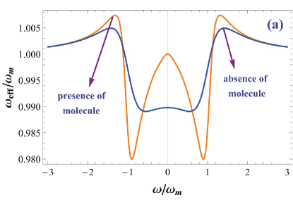
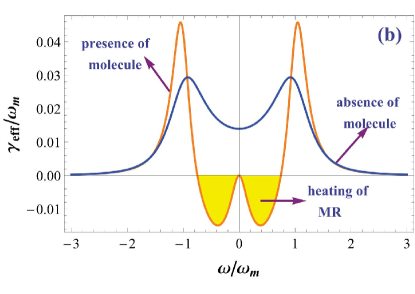
Figure 2: (Color online) (a) The normalized effective frequency $\omega_{eff}/\omega_{m}$ as a function of the normalized system response frequency $\omega/\omega_{m}$ at $\Delta_{p}/|\zeta_{0s}|=-\omega_{m}$ in presence and absence of the molecule. (b) The normalized effective damping parameter $\gamma_{eff}/\omega_{m}$ as a function of the normalized system response frequency $\omega/\omega_{m}$ at $\Delta_{p}/|\zeta_{0s}|=-\omega_{m}$ in presence and absence of the molecule. The cavity damping is assumed to be $\gamma_{f}=0.4\omega_{m}$, while the other parameters are $P_{c}=5$mW, $\omega_{m}/2\pi=10$MHz, $m=10$ng, $Q=50\times 10^{4}$, $d=100$nm, $\beta=0.013$, $\gamma_{a}=0.8\omega_{m}$ and $g=5$kHz.

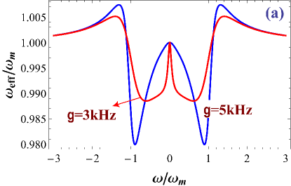
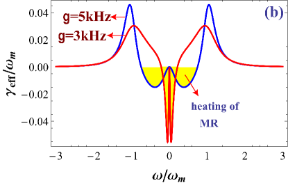
Figure 3: (Color online) (a) The normalized effective frequency $\omega_{eff}/\omega_{m}$ as a function of the normalized system response frequency $\omega/\omega_{m}$ for two different values of molecule-field coupling constant $g=3$kHz and $g=5$kHz. (b) The normalized effective damping parameter $\gamma_{eff}/\omega_{m}$ as a function of the normalized system response frequency $\omega/\omega_{m}$ for two different values of molecule-field coupling constant $g=3$kHz and $g=5$kHz. Here, we have assumed $\Delta_{p}/|\zeta_{0s}|=-\omega_{m}$ and the other parameters are the same as Fig. 2.

Fig. 2 shows the normalized effective frequency as a function of the normalized system response frequency $\omega/\omega_{m}$ at $\Delta_{p}/|\zeta_{0s}|=-\omega_{m}$ in presence and absence of the molecule in a case of $\zeta_{0}=-1$. The cavity damping is assumed to be $\gamma_{f}=0.4\omega_{m}$, while the other parameters are Teufel et al. (2011b): $P_{c}=5$mW, $\omega_{m}/2\pi=10$MHz, $m=10$ng, $Q=50\times 10^{4}$, $d=100$nm, $\beta=0.013$, $\gamma_{a}=0.8\omega_{m}$ and $g=5$kHz Rabl et al. (2006). We see that presence of the molecule potentially increases the effective frequency and damping parameter of the nanomechanical resonator. Further information can be found in Fig. 3, which shows the influence of the molecule-field coupling rate $g$ on the effective frequency and damping parameter. This figure confirms that, by increasing the parameter $g$, both parameters $\omega_{eff}$ and $\gamma_{eff}$ increase.

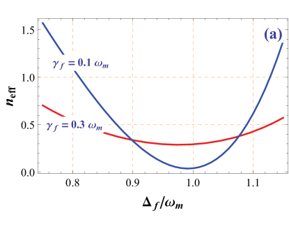
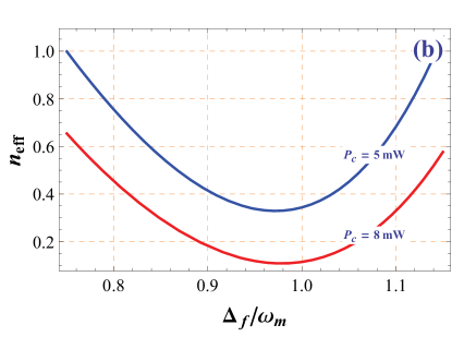
Figure 4: (Color online) (a) The effective mean excitation $n_{eff}$ versus the normalized effective detuning $\Delta_{f}/\omega_{m}$ for different values of the cavity damping rate $\gamma_{f}=0.1\omega_{m}$ and $\gamma_{f}=0.3\omega_{m}$. (b) The effective mean excitation $n_{eff}$ versus the normalized effective detuning $\Delta_{f}/\omega_{m}$ for different values of the driven power $P_{c}=5$mW and $P_{c}=8$mW. The molecular detuning has been fixed at $\Delta_{p}/|\zeta_{0}|=-\omega_{m}$, while the other parameters are $\omega_{m}/2\pi=10$MHz, $m=10$ng, $Q=50\times 10^{4}$, $d=100$nm, $\beta=0.013$, $g=10$kHz and the reservoir temperature is $T=0.2K$.

V GROUND STATE COOLING OF THE NANOMECHANICAL RESONATOR

In this section, we study the ground state cooling of the nanomechanical resonator coupled to the diatomic molecule in the steady state. We note that the current system is stable and reaches a steady state after a transient time if all the eigenvalues of the drift matrix A have negative real part. These stability conditions can be obtained by using the Routh-Hurwitz criteria Gradshteyn and Ryzhik . The mean energy of the nanomechanical resonator in the steady state is

$$U=\frac{\hbar\omega_{m}}{2}\Big{[}\langle\delta q^{2}\rangle+\langle\delta p^{2}\rangle\Big{]}=\frac{\hbar\omega_{m}}{2}(V_{11}+V_{22})\equiv\hbar\omega_{m}(n_{eff}+\frac{1}{2}),$$

where $V_{11}$ and $V_{22}$ are the first and second diagonal components of the stationary correlation matrix

$$V_{ij}=\int_{0}^{\infty}ds\int_{0}^{\infty}ds^{\prime}M_{ik}(s)M_{jl}(s^{\prime})D_{kl}(s-s^{\prime}),$$ (27)

where $\textbf{M}(t)=\exp(\textbf{A}t)$ and $\textbf{D}(s-s^{\prime})$ is the diffusion matrix given by Eq. (22). It is worth mentioning that, the nanomechanical resonator reaches its ground state if $n_{eff}\simeq 0$ or $V_{11}\equiv\langle\delta q^{2}\rangle\simeq 1/2$ and $V_{22}\equiv\langle\delta p^{2}\rangle\simeq 1/2$.

In Fig. 4(a) we have plotted the effective number of vibrational excitations $n_{eff}$ as a function of the normalized cavity detuning $\Delta_{f}/\omega_{m}$ for two different values of the cavity damping rate $\gamma_{f}$ in $\Delta_{p}/|\zeta_{0}|=-\omega_{m}$. The microwave cavity is assumed to work in frequency $\omega_{f}/2\pi=10$GHz which is driven by a microwave source with power $P_{c}=8$mW. We also have considered molecule $K_{2}$ with $\omega_{e}=17$THz, $D_{e}=8.1\times 10^{-20}$J, $\omega_{p}/2\pi=90$GHz Noggle (1996), and $g=10$kHz. Fig. 4 (a) shows that decreasing the cavity damping improves the cooling process for nanomechanical resonator. However, Fig. 4(b) describes the effect of the laser power $P_{c}$ on the ground state cooling of nanomechanical resonator. It is evident that the lower nanomechanical resonator excitation is obtained in the higher values of the input power.

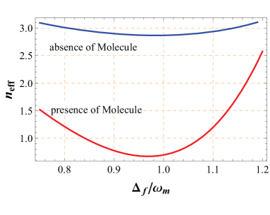
Figure 5: (Color online) Comparing the effective mean excitation $n_{eff}$ in presence and absence of the molecule for $g=10$kHz. The other parameters are the same as Fig. 4.

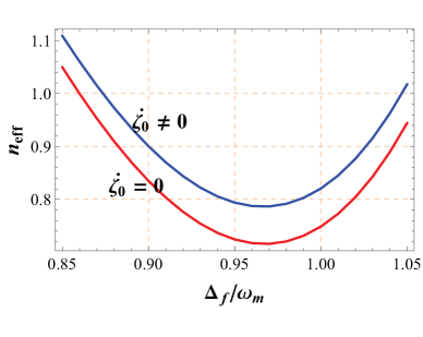
Figure 6: (Color online) The effective mean excitation $n_{eff}$ for two different regimes $\dot{\zeta}_{0}=0$ and $\dot{\zeta}_{0}\neq 0$ with $g=10$kHz. The other parameters are the same as Fig. 4.

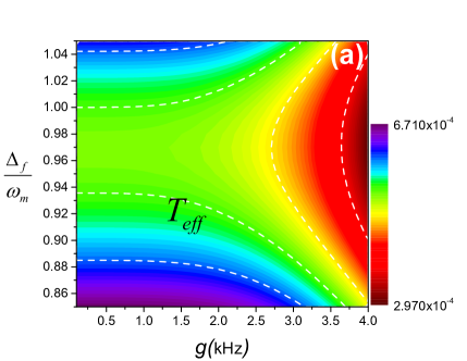
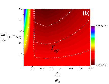
Figure 7: (Color online) (a) The effective temperature $T_{eff}$ versus normalized cavity field detuning $\Delta_{f}/\omega_{m}$ and molecule-field coupling contestant $g$. (b) The effective temperature $T_{eff}$ versus the molecule nonlinearity parameter $\hbar a^{2}/2\mu$ and the normalized molecule damping rate $\gamma_{p}/\omega_{m}$. The other parameters are the same as Fig. 4.

A more interesting situation is depicted in Fig. 5 which compares $n_{eff}$ in presence and absence of the molecule. This figure reveals that presence of the molecule potentially could improve the cooling process for the nanomechanical resonator. This figure is depicted for situation $\dot{\zeta}_{0}\neq 0$ which corresponds to the last line of Eq. (III.1). However, the excitation probability of a single molecule is usually assumed to be low i.e., $\zeta_{0}=\mathrm{cte}$ or $\dot{\zeta}_{0}\simeq 0$. This is valid in the low molecular excitation limit, i.e., when the molecule is initially prepared in its ground state and interaction with the cavity field does not effectively change the molecule excitation. This means that the single-molecule excitation probability should be much less than 1, i.e., $g^{2}\ll\Delta_{p}^{2}+\gamma_{p}^{2}$. In this regime, one can assume $\dot{\zeta}_{0}\simeq 0$, which is equivalent to ignoring the last differential equation in Eq. (III.1). In Fig. 6 we have plotted $n_{eff}$ versus the normalized detuning $\Delta_{f}/\omega_{m}$ for two different scenarios $\dot{\zeta}_{0}\simeq 0$ and $\dot{\zeta}_{0}\neq 0$. It is interesting that, in the case of the low molecular excitation limit i.e., $\dot{\zeta}_{0}\simeq 0$, one can reach lower temperature for nanomechanical resonator. In principle, this approximation is identical with the bosonization method proposed for atoms Genes et al. (2008a).

Now, we investigate the effect of the molecule parameters on the cooling of nanomechanical resonator in the low molecular excitation regime. The effective temperature of the nanomechanical resonator $T_{eff}=\frac{\hbar\omega_{m}}{\mathrm{k_{B}}\mathrm{ln}(1+1/n_{eff})}$ versus the normalized cavity detuning $\Delta_{f}/\omega_{m}$ and the molecule-field coupling rate $g$ is depicted in Fig. 7(a). As expected, the stronger coupling between the intracavity mode and the molecule leads to a lower temperature for nanomechanical resonator. Figure 7(b) shows $T_{eff}$ versus the molecule damping and parameter $\omega_{p}=\hbar a^{2}/2\mu$ in the fixed cavity detuning $\Delta_{f}=\omega_{m}$. This is interesting to mentioned that for $\gamma_{p}\gtrsim 0.12\omega_{m}$ by increasing the parameter $\omega_{p}$, which indicates the strength of molecule nonlinearity, the effective temperature decreases. However, the lowest nanomechanical resonator temperature is approached around $\gamma_{p}\simeq 0.25\omega_{m}$. On the other hand, for $\gamma_{p}\lesssim 0.12\omega_{m}$, increasing the parameter $\omega_{p}$ suppresses the cooling process of the nanomechanical resonator.

Finally, Fig. 8 shows the effective temperature $T_{eff}$ versus $\Delta_{f}/\omega_{m}$ in the presence of three different types of the diatomic molecules $\mathrm{HCl}$, $\mathrm{HI}$, and $\mathrm{NO}$ where each molecule is indicated by parameter $\omega_{e}/\sqrt{2D_{e}}$. Here, $\omega_{e}/\sqrt{2D_{e}}=4.7\times 10^{23}$ for $\mathrm{HCl}$, $\omega_{e}/\sqrt{2D_{e}}=4.41\times 10^{23}$ for $\mathrm{HI}$, and $\omega_{e}/\sqrt{2D_{e}}=2.5\times 10^{23}$ for $\mathrm{NO}$ Noggle (1996). It is evident that by increasing the value of $\omega_{e}/\sqrt{2D_{e}}$, which increases the width of potential well for constant $\mu$, we achieve a lower temperature for the nanomechanical resonator.

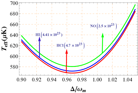
Figure 8: (Color online) The effective temperature $T_{eff}$ versus the normalized effective detuning $\Delta/\omega_{m}$ for three different molecules $\mathrm{HCl}$, $\mathrm{HI}$, and $\mathrm{NO}$. Here, $\omega_{e}/\sqrt{2D_{e}}=4.7\times 10^{23}$ for $\mathrm{HCl}$, $\omega_{e}/\sqrt{2D_{e}}=4.41\times 10^{23}$ for $\mathrm{HI}$, and $\omega_{e}/\sqrt{2D_{e}}=2.5\times 10^{23}$ for $\mathrm{NO}$. The other parameters are the same as Fig. 4.

We note that one of the realizations of the diatomic molecules are in DNA molecules Zdravković and Satarić (2012). It is well-known that a DNA molecule consists of two compatible chains. Chemical bonds between neighbouring nucleotides belonging to the same strands are strong covalent bonds, while nucleotides at a certain site $n$, belonging to the different strands, are connected through weak hydrogen interaction Peyrard and Bishop (1989); Dauxois (1991). Interaction between nucleotides at the same site belonging to different strands is modelled by a mechanical resonator energy.

VI CONCLUSIONS

In this paper, we have proposed a theoretical scheme for realization of tripartite coupling among a single mode of the microwave cavity, a single diatomic molecule, and the vibrational mode of a nanomechanical resonator. We have shown that, by describing the diatomic molecule with a Morse potential, a type of tripartite molecule-nanomechanical resonator-field coupling can be manifested. The dynamics of the hybrid system is studied by using the Fokker-Planck equation. We have focused our attention on the steady state of the system and, in particular, on the stationary quantum fluctuations of the system. By solving the linearized dynamics around the classical steady state we have found the effective frequency and the effective damping parameter of the nanomechanical resonator. We have seen that, in an experimentally accessible parameter regime, presence of the molecule modifies the effective frequency and the damping rate of the nanomechanical resonator. Moreover, we have studied the cooling of the nanomechanical resonator and have shown that presence of the diatomic molecule improves the efficiency of the cooling mechanism for the nanomechanical resonator. We have found that by increasing the coupling constant between the molecule and cavity field, the effective temperature of the nanomechanical resonator decreases. We have also discussed about the effect of molecular parameters on the temperature of the nanomechanical resonator. We have shown that, by increasing the molecule parameter $\omega_{e}/\sqrt{2D_{e}}$, one can reach lower temperatures for the nanomechanical resonator. The realization of such a scheme will open new opportunities for coupling between nanomechanical resonators and diatomic-like molecules such as DNA.

Appendix A Definition of variables in Eqs. (21) and (22)

$$G_{0s} = 2g\zeta_{0s},\,\,\Gamma_{0}=2\gamma_{p}\zeta_{0s},\,g^{R}=\sqrt{2}g\mathrm{Re}\zeta_{s},$$

$$g^{I} = \sqrt{2}g\mathrm{Im}\zeta_{s},\,\,\gamma_{p}^{R}=2\sqrt{2}\gamma_{p}\mathrm{Re}\zeta_{s},$$

$$\gamma_{p}^{I} = 2\sqrt{2}\gamma_{p}\mathrm{Im}\zeta_{s}+\sqrt{2}g\alpha_{s},$$ (28)

$$K_{1} = \sqrt{2}\left[2\gamma_{p}\mathrm{Re}\zeta_{s}-\mathrm{Im}(2\omega_{p}\zeta_{s}+2g\alpha_{s})\right],$$

$$K_{2} = \sqrt{2}\left[2\gamma_{p}\mathrm{Im}\zeta_{s}+\mathrm{Re}(2\omega_{p}\zeta_{s}+2g\alpha_{s})\right],$$

$$P = \langle\Gamma_{\zeta}\Gamma_{\zeta}\rangle+\langle\Gamma_{\zeta^{*}}\Gamma_{\zeta^{*}}\rangle,$$

$$M = -i\left[\langle\Gamma_{\zeta}\Gamma_{\zeta}\rangle-\langle\Gamma_{\zeta^{*}}\Gamma_{\zeta^{*}}\rangle\right],\,\,Q=\langle\Gamma_{\zeta_{0}}\Gamma_{\zeta_{0}}\rangle.$$

Appendix B Definition of variables in Eqs. (25) and (26)

$$\Lambda = \left(\Omega_{T}\Omega_{Y^{\prime}}-\Gamma_{T}\Gamma_{Y^{\prime}}\right)(\Omega_{X}\Omega_{Y}-\Gamma_{X}\Gamma_{Y}-\Omega_{X^{\prime}}\Omega_{Y^{\prime}}+\Gamma_{X^{\prime}}\Gamma_{Y^{\prime}})$$

$$+ (\Omega_{T}\Gamma_{Y^{\prime}}+\Gamma_{T}\Omega_{Y^{\prime}}+\Gamma_{T}\Omega_{Y^{\prime}})(\Omega_{X}\Gamma_{Y}+\Omega_{Y}\Gamma_{X}-\Omega_{X^{\prime}}\Gamma_{Y^{\prime}}-\Omega_{Y^{\prime}}\Gamma_{X^{\prime}}),$$

$$\Lambda^{\prime} = (\Omega_{T}\Gamma_{Y^{\prime}}+\Omega_{Y}\Gamma_{T})(\Omega_{X}\Omega_{Y}-\Gamma_{X}\Gamma_{Y}-\Omega_{X^{\prime}}\Omega_{Y^{\prime}}+\Gamma_{X^{\prime}}\Gamma_{Y^{\prime}})$$

$$- (\Omega_{T}\Omega_{Y^{\prime}}-\Gamma_{T}\Gamma_{Y^{\prime}})(\Omega_{X}\Omega_{Y}+\Gamma_{X}\Gamma_{Y})-\Omega_{X^{\prime}}\Omega_{Y^{\prime}}-\Omega_{Y^{\prime}}\Gamma_{X^{\prime}}),$$

$$\Omega_{T} = \Omega_{p}^{2}+\Gamma_{0}^{2}-\left(\frac{K_{2}\gamma_{p}^{I}}{\omega}-\omega\right)\left(\frac{K_{1}\gamma_{p}^{R}}{\omega}-\omega\right)+\left(\frac{K_{2}\gamma_{p}^{R}}{\omega}\right)\left(\frac{K_{1}\gamma_{p}^{I}}{\omega}\right),$$

$$\Gamma_{T} = \frac{K_{1}\gamma_{p}^{I}\Omega_{p}}{\omega}-\frac{K_{2}\gamma_{p}^{R}\Omega_{p}}{\omega}-\Gamma_{0}\left(\frac{K_{1}\gamma_{p}^{R}}{\omega}-\omega\right)-\Gamma_{0}\left(\frac{K_{2}\gamma_{p}^{I}}{\omega}-\omega\right),$$

$$\Omega_{X} = \gamma_{f}\Omega_{T}+\omega\Gamma_{T}-gG_{0s}\Gamma_{0}+g\left(\frac{K_{2}\gamma_{p}^{R}}{\omega}\right)\left(\frac{K_{1}g^{I}}{\omega}\right)+g\left(\frac{K_{2}g^{I}}{\omega}\right)\left(\frac{K_{1}\gamma_{p}^{R}}{\omega}-\omega\right),$$ (29)

$$\Gamma_{X} = \gamma_{f}\Gamma_{T}-\omega\Omega_{T}+g\Omega_{p}\left(\frac{K_{1}g^{I}}{\omega}\right)-gG_{0s}\left(\frac{K_{1}\gamma_{p}^{R}}{\omega}-\omega\right)+g\Gamma_{0}\left(\frac{K_{2}g^{I}}{\omega}\right),$$

$$\Omega_{Y} = \gamma_{f}\Omega_{T}+\omega\Gamma_{T}-gG_{0s}\Gamma_{0}+g\left(\frac{K_{1}\gamma_{p}^{I}}{\omega}\right)\left(\frac{K_{2}g^{R}}{\omega}\right)+g\left(\frac{K_{1}g^{R}}{\omega}\right)\left(\frac{K_{2}\gamma_{p}^{I}}{\omega}-\omega\right),$$

$$\Gamma_{Y} = \gamma_{f}\Gamma_{T}-\omega\Omega_{T}+g\Omega_{p}\left(\frac{K_{2}g^{R}}{\omega}\right)-gG_{0s}\left(\frac{K_{2}\gamma_{p}^{I}}{\omega}-\omega\right)+g\Gamma_{0}\left(\frac{K_{1}g^{R}}{\omega}\right),$$

$$\Omega_{X^{\prime}} = -\Delta\Omega_{T}+g\Omega_{p}G_{0s}+g\left(\frac{K_{1}\gamma_{p}^{I}}{\omega}\right)\left(\frac{K_{2}g^{I}}{\omega}\right)-g\left(\frac{K_{1}g^{I}}{\omega}\right)\left(\frac{K_{2}\gamma_{p}^{I}}{\omega}-\omega\right),$$

$$\Gamma_{X^{\prime}} = -\Delta\Gamma_{T}-g\Omega_{p}\left(\frac{K_{2}g^{I}}{\omega}\right)+gG_{0s}\left(\frac{K_{1}\gamma_{p}^{I}}{\omega}\right)-g\Gamma_{0}\left(\frac{K_{1}g^{I}}{\omega}\right),$$

$$\Omega_{Y^{\prime}} = \Delta\Omega_{T}-g\Omega_{p}G_{0s}+g\left(\frac{K_{2}g^{R}}{\omega}\right)\left(\frac{K_{1}\gamma_{p}^{R}}{\omega}-\omega\right)-g\left(\frac{K_{1}g^{R}}{\omega}\right)\left(\frac{K_{2}\gamma_{p}^{R}}{\omega}\right),$$

$$\Gamma_{Y^{\prime}} = \Delta\Gamma_{T}+g\Omega_{p}\left(\frac{K_{1}g^{R}}{\omega}\right)+gG_{0s}\left(\frac{K_{2}\gamma_{p}^{R}}{\omega}\right)-g\Gamma_{0}\left(\frac{K_{2}g^{R}}{\omega}\right).$$

References

• Aspelmeyer et al. (2014) M. Aspelmeyer, T. J. Kippenberg,  and F. Marquardt, Rev. Mod. Phys. 86, 1391 (2014).
• Chen (2013) Y. Chen, J. Phys. B: At. Mol. Opt. Phys. 46, 104001 (2013).
• Cleland (2003) A. N. N. Cleland, Foundations of Nanomechanics (Springer, Berlin, 2003).
• Kleckner and Bouwmeester (2006) D. Kleckner and D. Bouwmeester, Nature 444, 75 (2006).
• Poggio et al. (2007) M. Poggio, C. Degen, H. Mamin,  and D. Rugar, Phys. Rev. Lett. 99, 017201 (2007).
• Teufel et al. (2008) J. Teufel, J. Harlow, C. Regal,  and K. Lehnert, Phys. Rev. Lett. 101, 197203 (2008).
• Arcizet et al. (2006) O. Arcizet, P. F. Cohadon, T. Briant, M. Pinard,  and A. Heidmann, Nature 444, 71 (2006).
• Teufel et al. (2011a) J. D. Teufel, T. Donner, D. Li, J. W. Harlow, M. S. Allman, K. Cicak, A. J. Sirois, J. D. Whittaker, K. W. Lehnert,  and R. W. Simmonds, Nature 475, 359 (2011a).
• Cohadon et al. (1999) P. F. Cohadon, A. Heidmann,  and M. Pinard, Phys. Rev. Lett. 83, 3174 (1999).
• Gigan et al. (2006) S. Gigan, H. Böhm, M. Paternostro, F. Blaser, G. Langer, J. Hertzberg, K. Schwab, D. Bäuerle, M. Aspelmeyer,  and A. Zeilinger, Nature 444, 67 (2006).
• Brown et al. (2007) K. Brown, J. Britton, R. Epstein, J. Chiaverini, D. Leibfried,  and D. Wineland, Phys. Rev. Lett. 99, 137205 (2007).
• Xue et al. (2007) F. Xue, Y. Wang, Y. X. Liu,  and F. Nori, Phys. Rev. B 76, 205302 (2007).
• Zhang et al. (2009) J. Zhang, Y. Liu,  and F. Nori, Phys. Rev. A 79, 052102 (2009).
• Xiang et al. (2013) Z. L. Xiang, S. Ashhab, J. Q. You,  and F. Nori, Rev. Mod. Phys. 85, 623 (2013).
• Hammerer et al. (2009) K. Hammerer, M. Wallquist, C. Genes, M. Ludwig, F. Marquardt, P. Treutlein, P. Zoller, J. Ye,  and H. Kimble, Phys. Rev. Lett. 103, 063005 (2009).
• Wallquist et al. (2010) M. Wallquist, K. Hammerer, P. Zoller, C. Genes, M. Ludwig, F. Marquardt, P. Treutlein, J. Ye,  and H. Kimble, Phys. Rev. A 81, 023816 (2010).
• Chang et al. (2009) Y. Chang, H. Ian,  and C. Sun, J. Phys. B: At. Mol. Opt. Phys. 42, 215502 (2009).
• Breyer and Bienert (2012) D. Breyer and M. Bienert, Phys. Rev. A 86, 053819 (2012).
• Barzanjeh et al. (2011) S. Barzanjeh, M. Naderi,  and M. Soltanolkotabi, Phys. Rev. A 84, 063850 (2011).
• Ian et al. (2008) H. Ian, Z. Gong, Y.-x. Liu, C. Sun,  and F. Nori, Phys. Rev. A 78, 013824 (2008).
• Schleier-Smith et al. (2011) M. H. Schleier-Smith, I. D. Leroux, H. Zhang, M. A. Van Camp,  and V. Vuletić, Phys. Rev. Lett. 107, 143005 (2011).
• Genes et al. (2008a) C. Genes, D. Vitali,  and P. Tombesi, Phys. Rev. A 77, 050307 (2008a).
• Tian and Zoller (2004) L. Tian and P. Zoller, Phys. Rev. Lett. 93 (2004).
• Bhattacharya et al. (2010) M. Bhattacharya, S. Singh, P.-L. Giscard,  and P. Meystre, Laser Phys. 20, 57 (2010).
• Singh et al. (2008) S. Singh, M. Bhattacharya, O. Dutta,  and P. Meystre, Phys. Rev. Lett. 101, 263603 (2008).
• Ciaramicoli et al. (2007) G. Ciaramicoli, I. Marzoli,  and P. Tombesi, Phys. Rev. A 75, 032348 (2007).
• Vitali et al. (2007) D. Vitali, P. Tombesi, M. J. Woolley, A. C. Doherty,  and G. J. Milburn, Phys. Rev. A 76, 042336 (2007).
• Kielpinski et al. (2012) D. Kielpinski, D. Kafri, M. Woolley, G. Milburn,  and J. Taylor, Phys. Rev. Lett. 108, 130504 (2012).
• Daniilidis and Häffner (2013) N. Daniilidis and H. Häffner, Annu. Rev. Condens. Matter Phys. 4, 83 (2013).
• Gangopadhyay and Ray (1990) G. Gangopadhyay and D. S. Ray, Phys. Rev. A 41, 6429 (1990).
• Gangopadhyay and Ray (1991) G. Gangopadhyay and D. S. Ray, Phys. Rev. A 43, 6424 (1991).
• Dong et al. (2003) S.-H. Dong, Y. Tang,  and G.-H. Sun, Phys. Lett. A 320, 145 (2003).
• Angelova and Hussin (2008) M. Angelova and V. Hussin, J. Phys. A: Math. Theor. 41, 304016 (2008).
• Noggle (1996) J. H. Noggle, Physical Chemistry, 3rd Edition (New York, 1996).
• Schleich (2001) W. P. Schleich, Quantum optics in phase space (WILEY-VCH, 2001).
• Gardiner and Zoller (2004) C. Gardiner and P. Zoller, Quantum noise: a handbook of Markovian and non-Markovian quantum stochastic methods with applications to quantum optics, Vol. 56 (Springer, 2004).
• Holmes and Milburn (2009) C. Holmes and G. Milburn, Fortschritte der Physik 57, 1052 (2009).
• Genes et al. (2008b) C. Genes, D. Vitali, P. Tombesi, S. Gigan,  and M. Aspelmeyer, Phys. Rev. A 77, 033804 (2008b).
• Teufel et al. (2011b) J. Teufel, T. Donner, D. Li, J. Harlow, M. Allman, K. Cicak, A. Sirois, J. Whittaker, K. Lehnert,  and R. Simmonds, Nature 475, 359 (2011b).
• Rabl et al. (2006) P. Rabl, D. DeMille, J. Doyle, M. Lukin, R. Schoelkopf,  and P. Zoller, Phys. Rev. Lett 97, 033003 (2006).
• (41) I. Gradshteyn and I. Ryzhik, Table of Integrals, Series and Products (Academic, Orlando, 1980).
• Zdravković and Satarić (2012) S. Zdravković and M. V. Satarić, J. Biosci 37, 613 (2012).
• Peyrard and Bishop (1989) M. Peyrard and A. Bishop, Phys. Rev. Lett. 62 (1989).
• Dauxois (1991) T. Dauxois, Phys. Rev. Lett. 159, 390 (1991).