The rate of linear convergence of the
Douglas–Rachford algorithm for subspaces
is the cosine of the Friedrichs angle
Heinz H. Bauschke,
J.Y. Bello Cruz, Tran T.A. Nghia,
Hung M. Phan, and
Xianfu Wang
Mathematics, University of British
Columbia, Kelowna, B.C. V1V 1V7, Canada. E-mail:
heinz.bauschke@ubc.ca.IME, Federal University of Goias,
Goiania, G.O. 74001-970, Brazil. E-mail:
yunier.bello@gmail.com.Mathematics, University of British Columbia, Kelowna, B.C. V1V 1V7, Canada. E-mail: nghia.tran@ubc.ca.Mathematics, University of British Columbia, Kelowna, B.C. V1V 1V7, Canada. E-mail: hung.phan@ubc.ca.Mathematics, University of British Columbia,
Kelowna, B.C. V1V 1V7, Canada. E-mail:
shawn.wang@ubc.ca.
(December 20, 2013)
Abstract
The Douglas–Rachford splitting algorithm is a
classical optimization method that has found many applications.
When specialized to two normal cone operators, it yields
an algorithm for finding a point in the intersection of
two convex sets.
This method for solving feasibility problems
has attracted a lot of attention due to its
good performance even in nonconvex settings.
In this paper,
we consider the Douglas–Rachford algorithm
for finding a point in the intersection of two subspaces.
We prove that the method converges strongly to the projection of the
starting point onto the intersection. Moreover,
if the sum of the two subspaces is closed,
then the convergence is linear with the rate being the cosine
of the Friedrichs angle between the subspaces.
Our results improve upon existing results in three ways:
First, we identify the location of the limit and thus reveal
the method as a best approximation algorithm;
second, we quantify the rate of convergence, and third,
we carry out our analysis in general (possibly
infinite-dimensional) Hilbert space.
We also provide various examples as well as a
comparison with the classical method of alternating projections.
Keywords:
Douglas–Rachford splitting method,
firmly nonexpansive,
Friedrichs angle,
linear convergence,
method of alternating projections,
normal cone operator,
subspaces,
projection operator.
1 Introduction
Throughout this paper,
we assume that
(1)
is a real Hilbert space
with inner product and induced norm
.
Let and be closed convex subsets of such that
.
The convex feasibility problem is to find a point in
. This is a basic problem in the natural sciences and
engineering (see, e.g., [5], [15], and [16]) —
as such, a plethora of algorithms based on the
nearest point mappings (projectors) and have been
proposed to solve it.
One particularly popular method is the Douglas–Rachford
splitting algorithm [19] which utilizes the
the Douglas–Rachford splitting operator
(2)
and to generate the sequence by
(3)
While the sequence may or may not converge to a
point in , the projected (“shadow”) sequence
(4)
always converges (weakly) to a point in
(see [27], [29], [4], [7]).
The Douglas–Rachford algorithm has been applied very
successfully to various problems where and are not
necessarily convex, even though the supporting formal theory is
far from being complete (see, e.g., [1], [8], and
[21]).
Very recently, Hesse, Luke and Neumann [24] (see also
[23]) considered
projection methods for the (nonconvex) sparse affine feasibility
problem. Their paper highlights the importance of understanding
the Douglas–Rachford algorithm for the case when and
are closed subspaces of ; their basic convergence
result is the following.
Fact 1.1(Hesse–Luke–Neumann)
(See [24, Theorem 4.6].)
Suppose that is finite-dimensional and
and are subspaces of .
Then the sequence generated by (3) converges to a
point in with a linear rate111Recall that
linearly or with a linear rate if is bounded..
The aim of this paper is three-fold.
We complement Fact 1.1 by providing the following:
•
We identify the limit of the shadow sequence as
; consequently and somewhat surprisingly,
the Douglas–Rachford method in this
setting not only solves a feasibility problem but actually a
best approximation problem.
•
We quantify the rate of convergence — it turns out to be the cosine of the
Friedrichs angle between and ; moreover, our estimate is sharp.
•
Our analysis is carried out in general (possibly
infinite-dimensional) Hilbert space.
The paper is organized as follows.
In Sections 2 and 3,
we collect various auxiliary results to
facilitate the proof of the main results (Theorem 4.1 and Theorem 4.3)
in Section 4.
In Section 5, we analyze the Douglas–Rachford algorithm
for two lines in the Euclidean plane.
The results obtained are used in Section 6 for
an infinite-dimensional construction illustrating the lack of
linear convergence.
In Section 7, we compare
the Douglas–Rachford algorithm to the method of alternating
projections.
We report on numerical experiments in Section 8,
and conclude the paper in Section 9.
Notation is standard and follows largely [7].
We write to indicate that the terms of the Minkowski sum satisfy .
2 Auxiliary results
In this section, we collect various results to ease the derivation
of the main results.
2.1 Firmly nonexpansive mappings
It is well known (see [27], [20], or [8])
that the Douglas–Rachford operator (see
(2)) is firmly nonexpansive, i.e.,
(5)
The following result will be useful in our analysis.
Fact 2.1
(See [7, Corollary 5.16 and Proposition 5.27], or
[11, Theorem 2.2], [3] and [14].)
Let be linear and firmly nonexpansive, and let
.
Then .
2.2 Products of projections and the Friedrichs angle
Unless otherwise stated, we assume from now on that
(6)
and are closed subspaces of .
The proof of the following useful fact
can be found in [18, Lemma 9.2]:
(7)
Our main results are formulated using the notion of the Friedrichs
angle between and . Let us review the definition and
provide the key results which are needed in the sequel.
Definition 2.2
The cosine of the Friedrichs angle
between and is
(8)
We write for if we emphasize the subspaces
utilized.
Fact 2.3(fundamental properties of the Friedrichs angle)
Let . Then the following hold:
(i)
is closed
.
(ii)
.
(iii)
.
(iv)
(Aronszajn–Kayalar–Weinert).
Proof. (i):
See [17, Theorem 13]
(ii):
See [17, Theorem 16]
(iii):
See [18, Lemma 9.5(7)] and (ii) above.
(iv):
See [18, Theorem 9.31] (or the original works
[2] and [26]).
(v):
Since and are firmly nonexpansive, so is their convex combination
, which equals by (iv).
It is clear that is self-adjoint.
(vi):
It follows
from Proposition 3.4(i)&(ii) that
, which yields the first equality.
Replacing and by
and , respectively, followed by expanding and
simplifying results in the second equality. The last equality is
proved analogously.
Parts of our next result were also obtained in [23] and
[24] when is finite-dimensional.
Proposition 3.6
Let .
Then the following hold:
(i)
.
(ii)
.
(iii)
.
(iv)
.
(v)
.
Proof. (i):
Set and . Then .
Combining [6, Example 2.7 and Corollary 5.5(iii)] yields
.
By [11, Lemma 2.1], we have .
Since and are firmly nonexpansive, and , we apply
[7, Corollary 4.3 and Corollary 4.37]
to deduce that
.
(iv): Clearly, . Furthermore,
by [11, Lemma 3.12].
(v):
First, (iii) and (7) imply
.
This and (iv) give the remaining equalities.
4 Main result
We now are ready for our main results concerning the dynamical
behaviour of the Douglas–Rachford iteration.
Theorem 4.1(powers of )
Let , and let . Then
(18a)
(18b)
and
(19)
Proof. Set
(20)
and observe that the second equality is justified
since .
Since is (firmly) nonexpansive and normal
(see Proposition 3.5(iii)),
it follows from [11, Lemma 3.15(i)] that
We are now ready for our main result.
Note that item (i) is the counterpart of
Fact 2.3(iv) for the Douglas–Rachford algorithm.
Theorem 4.3(shadow powers of )
Let , and let .
Then the following hold:
(i)
.
(ii)
.
(iii)
.
Proof. (i):
Note that .
It follows that .
Hence, using Proposition 4.2(v), we have
and thus
by Lemma 2.4.
It follows likewise from Proposition 4.2(vi) and
Fact 2.3(iv) that
.
Thus, we have .
The proof of is analogous.
Combining this with Fact 2.3(iii) and
(18a), we get
.
Corollary 4.4(linear convergence)
We have
,
, and
.
If is closed,
then convergence of these sequences is linear with rate .
Proof. Corollary 3.1,
Proposition 3.6(iii)&(v) and
(7) imply
and analogously
.
Recall from
Fact 2.3(i)
that is closed if and only if .
The conclusion is thus clear from Theorem 4.3(iii).
A translation argument gives the following result (see also
[9, Theorem 3.17] for an earlier related result).
Corollary 4.5(affine subspaces)
Suppose that and are closed affine subspaces
of such that , and let .
Then
(33)
If is closed,
then the convergence is linear with rate .
5 Two lines in the Euclidean plane
We present some geometric results concerning the lines in the
plane which will not only be useful later but which also illustrate
the results of the previous sections.
In this section, we assume that , and we set
(34)
Define the (counter-clockwise) rotator by
(35)
and note that .
Now let ,
and suppose that
(36)
Then
(37)
By, e.g., [7, Proposition 28.2(ii)],
.
In terms of matrices, we thus have
(38)
Consequently,
the corresponding Douglas–Rachford splitting operator
is
(39a)
(39b)
Thus,
,
(40)
and
(41)
Furthermore,
(42)
and thus
(43)
6 An example without linear rate of convergence
In this section, let us assume that our underlying Hilbert space is
.
It will be more suggestive to use boldface letters
for vectors lying in, and operators acting on, .
Thus,
(44)
and we write is for a generic vector in .
Suppose that is a sequence of angles in
with .
We set .
We will use notation and results
from Section 5.
We assume that
(45)
and that
(46)
Then
(47)
The Douglas–Rachford splitting operator is
(48)
Now let and .
Assume further that is infinite.
Then there exists such that
and
.
Hence
(49)
consequently,
(50)
, but not linearly with
rate .
Let us now assume in addition that
and and
.
Then there exists and
such that . Hence, for every , we have
(51)
thus,
(52)
, but not linearly with
rate .
In summary, these constructions illustrate that
when the Friedrichs angle is zero, then
one cannot expect linear convergence of the
(projected) iterates of the Douglas–Rachford splitting operator.
7 Comparison with the method of alternating projections
Let us now compare our main results (Theorems 4.1 and
4.3)
with the method of alternating projections, for which
the following fundamental result is well known.
In Fact 7.1, the rate is best possible (see
Fact 2.3(iv) and the
results and comments in [18, Chapter 9]),
and if the Friedrichs
angle is 0, then slow convergence may occur
(see, e.g., [10]).
From Theorem 4.1, Corollary 4.4, and Fact 7.1, we see that
the rate of convergence of to and,
a fortiori, of to ,
is clearly slower than the rate of convergence of
to .
In other words, the Douglas–Rachford splitting method
appears to be twice as slow as the method
of alternating projections.
While this is certainly the case for the iterates ,
the actual iterates of interest, namely , in
practice often (somewhat paradoxically) make striking
non-monotone progress.
Let us illustrate this using the set up of Section 5
the notation and results of which we will utilize.
Consider first (41) and (43) with
and .
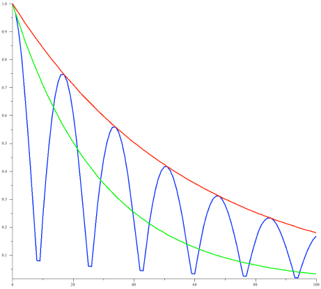
In Figure 1, we show the first 100 iterates of
the sequences
(red line),
(blue line), and
(green line). The sequences and
, which are decreasing,
represent the distance of the iterates to
, the unique solution of the problem.
While decreases
faster than , the sequence of “shadows”
exhibits a curious non-monotone
“rippling” behaviour
— it may be quite close to the solution soon after
the iteration starts!
Figure 1:
The distance of the first 100 terms of the sequences
(red), (blue), and
(green) to the
unique solution.
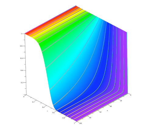
We next show in
Figure 2 and Figure 3
the first terms of
and , where
is
parametrized to exhibit more clearly the behaviour for small
angles. Clearly, and as predicted, smaller angles correspond to
slower rates of convergence.
Figure 2:
The distance of the first 100 terms of the sequence
to the unique solution when the angle ranges
between and .
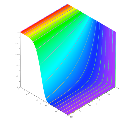
Figure 3:
The distance of the first 100 terms of the sequence
to the unique solution when the angle ranges
between and .
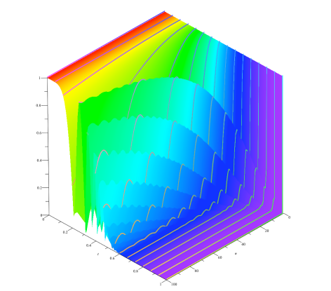
In Figure 4, we depict the “shadow sequence” .
Observe again the “rippling” phenomenon. While the situation of two lines
appears at first to be quite special, it turns out that the same
“rippling” also arises in a quite different setting; see [12, Figures 4 and 6].
Figure 4:
The distance of the first 100 terms of the “shadow” sequence
to the unique solution when the angle ranges
between and .
The figures in this section were prepared in Maple™ (see [28]).
8 Numerical experiments
In this section, we compare
the Douglas–Rachford method (DRM) to the method
of alternating projections (MAP)
for finding .
Our numerical set up is as follows.
We assume that , and we randomly
generated pairs of subspaces and of such that .
We then chose 10 random starting points, each with Euclidean norm .
This resulted in a total of 1,000 instances for each algorithm.
Note that the sequences to monitor are
(54)
for DRM and for MAP, respectively.
Our stopping criterion tolerance was set to
(55)
We investigated two different stopping criteria, which we detail
and discuss in the following two sections.
8.1 Stopping criterion based on the true error
We terminated the algorithm when the current iterate
of the monitored sequence satisfies
(56)
for the first time.
Note that in applications, we typically would not have access to
this information but here we use it to see the true performance
of the two methods.
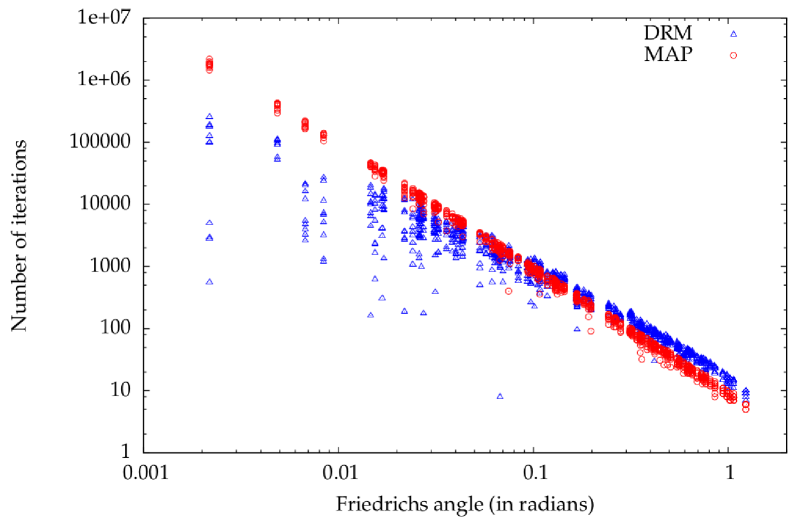
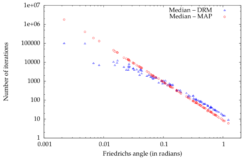
In Figure 5 and Figure 6, the horizontal axis
represents the Friedrichs angle between the subspaces and the vertical axis
represents the number of iterations. Results for all 1,000 runs are
presented in Figure 5, while we show the median
in Figure 6.
From the figures, we see that DRM is generally faster
than MAP
when the Friedrichs angle .
In the opposite case, MAP is faster.
This can be interpreted as follows. Since DRM converges with
linear rate while MAP does with rate , we expect that
MAP performs better when is small, i.e., is large.
But when the Friedrichs angle is small, the “rippling” behaviour of DRM
appears to manifest itself (see also Figure 1).
Note that MAP is not much faster than DRM, which suggests DRM as the better
overall choice.
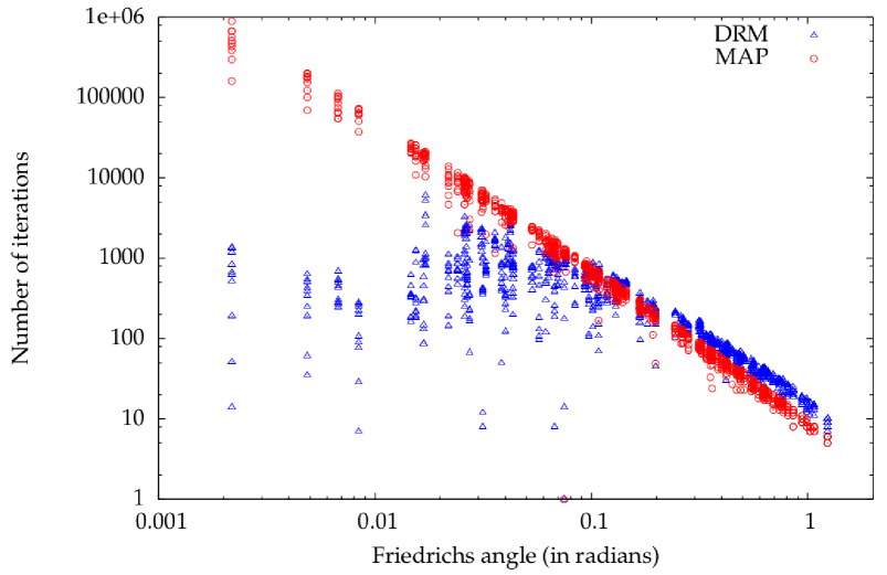
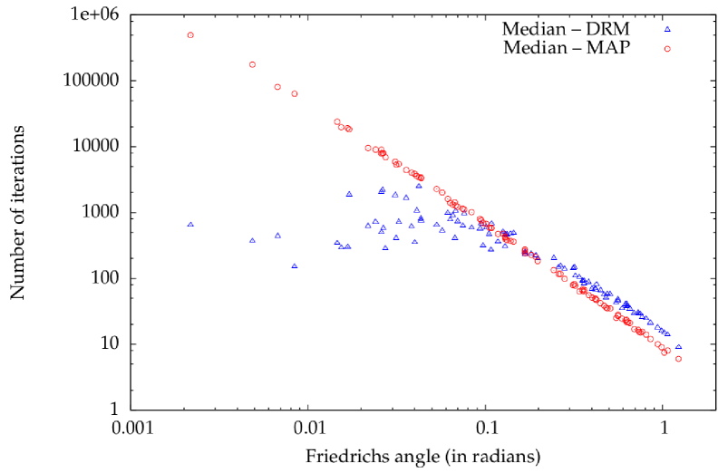
8.2 Stopping criterion based on individual distances
In practice, it is not always possible to obtain the true error.
Thus, we utilized a reasonable alternative stopping criterion, namely when
the monitored sequence satisfies
(57)
for the first time.
Figure 7: Max distance criterionFigure 8: Max distance criterion
Figures 7 and 8 show the results
when we use the max distance criterion with the same data.
The behaviour is similar to the experiments with the true error criterion.
The figures in this section were computed with the help of
Julia (see [25]) and Gnuplot (see
[22]).
9 Conclusion
We completely analyzed the Douglas–Rachford splitting method for the
important case of two subspaces. We determined the limit and the sharp rate
of convergence. Lack of linear convergence was illustrated by an example in
. Finally, we compared this method to the method of alternating
projections and found the Douglas–Rachford method to be faster when the
Friedrichs angle between the subspaces is small.
Acknowledgments
HHB was partially supported by a Discovery Grant and an Accelerator
Supplement of the Natural Sciences and Engineering
Research Council of Canada (NSERC) and by the Canada Research Chair Program.
JYBC was partially supported by CNPq and by projects UNIVERSAL and CAPES-MES-CUBA 226/2012. TTAN was partially supported by a postdoctoral
fellowship of the Pacific Institute for the Mathematical Sciences
and by NSERC grants of HHB and XW.
HMP was partially supported by NSERC grants of HHB and XW. XW was partially supported by a Discovery Grant of NSERC.
References
[1]
F.J. Aragón Artacho, J.M. Borwein, and M.K. Tam,
Recent results on Douglas-Rachford methods for combinatorial
optimization problems,
Journal of Optimization Theory and Applications, in press.
DOI 10.1007/s10957-013-0381-x
[2]
N. Aronszajn,
Theory of reproducing kernels,
Transactions of the AMS 68 (1950), 337–404.
[3]
J.B. Baillon, R.E. Bruck and S. Reich,
On the asymptotic behavior of nonexpansive mappings and semigroups
in Banach spaces,
Houston Journal of Mathematics 4(1) (1978), 1–9.
[4]
H.H. Bauschke,
New demiclosedness principles for (firmly) nonexpansive
operators,
Computational and Analytical Mathematics, Chapter 2,
Springer, 2013.
[5]
H.H. Bauschke and J.M. Borwein,
On projection algorithms for solving convex feasibility problems,
SIAM Review 38(3) (1996), 367–426.
[6]
H.H. Bauschke, R.I. Boţ, W.L. Hare, and W.M. Moursi,
Attouch–Théra duality revisited: paramonotonicity and operator
splitting,
Journal of Approximation Theory 164 (2012), 1065–1084.
[7]
H.H. Bauschke and P.L. Combettes,
Convex Analysis and Monotone Operator Theory in Hilbert Spaces,
Springer, 2011.
[8]
H.H. Bauschke, P.L. Combettes, and D.R. Luke,
Phase retrieval, error reduction algorithm, and
Fienup variants: a view from convex optimization,
Journal of the Optical Society of America 19(7) (2002),
1334–1345.
[9]
H.H. Bauschke, P.L. Combettes, and D.R. Luke,
Finding best approximation pairs relative to two closed convex sets in
Hilbert spaces,
Journal of Approximation Theory 127 (2004),
178–192.
[10]
H.H. Bauschke, F. Deutsch, and H. Hundal,
Characterizing arbitrarily slow convergence in the method of
alternating projections,
International Transactions in Operational Research 16
(2009), 413–425.
[11]
H.H. Bauschke, F. Deutsch, H. Hundal, and S.-H. Park,
Accelerating the convergence of the method of alternating projections,
Transactions of the AMS 355(9)
(2003),
3433–3461.
[12]
H.H. Bauschke and V.R. Koch,
Projection Methods: Swiss Army Knives for Solving Feasibility and
Best Approximation Problems with Halfspaces,
in Infinite Products and Their Applications, in press.
[13]
J.M. Borwein and M.K. Tam,
A cyclic Douglas–Rachford iteration scheme,
Journal of Optimization Theory and Applications, in press.
DOI 10.1007/s10957-013-0381-x
[14]
R.E. Bruck and S. Reich,
Nonexpansive projections and resolvents of accretive operators in Banach
spaces,
Houston Journal of Mathematics 3(4) (1977), 459–470.
[15]
Y. Censor and S.A. Zenios,
Parallel Optimization,
Oxford University Press, 1997.
[16]
P.L. Combettes,
The foundations of set theoretic estimation,
Proceedings of the IEEE 81(2) (1993), 182–208.
[17]
F. Deutsch,
The angle between subspaces of a Hilbert space,
in Approximation Theory, Wavelets and Applications,
S.P. Singh (editor), Kluwer, 1995, pp. 107–130.
[18]
F. Deutsch,
Best Approximation in Inner Product Spaces,
Springer, 2001.
[19]
J. Douglas and H.H. Rachford,
On the numerical solution of heat conduction problems
in two and three space variables,
Transactions of the AMS 82 (1956), 421–439.
[20]
J. Eckstein and D.P. Bertsekas,
On the Douglas-Rachford splitting method
and the proximal point algorithm for maximal monotone
operators,
Mathematical Programming (Series A) 55 (1992), 293–318.
[21]
V. Elser, I. Rankenburg, and P. Thibault,
Searching with iterated maps,
Proceedings of the National Academy of Sciences 104(2)
(2007), 418–423.
[22]
GNU Plot, http://sourceforge.net/projects/gnuplot
[23]
R. Hesse and D.R. Luke,
Nonconvex notions of regularity and convergence
of fundamental algorithms for feasibility problems,
SIAM Journal on Optimization 23 (2013), 2397–2419.
[24]
R. Hesse, D.R. Luke, and P. Neumann,
Projection methods for sparse affine feasibility:
results and counterexamples,
http://arxiv.org/abs/1307.2009, July 2013.
[25]
The Julia language, http://julialang.org/
[26]
S. Kayalar and H. Weinert,
Error bounds for the method of alternating projections,
Mathematics of Control, Signals, and Systems 1 (1996), 43–59.
[27]
P.-L. Lions and B. Mercier, Splitting algorithms for the sum
of two nonlinear operators,
SIAM Journal on Numerical Analysis 16 (1979), 964–979.