Normality condition in elasticity

Abstract

Strong local minimizers with surfaces of gradient discontinuity appear in variational problems when the energy density function is not rank-one convex. In this paper we show that stability of such surfaces is related to stability outside the surface via a single jump relation that can be regarded as interchange stability condition. Although this relation appears in the setting of equilibrium elasticity theory, it is remarkably similar to the well known normality condition which plays a central role in the classical plasticity theory.

1 Introduction

In the studies of necessary conditions for singular minimizers containing surfaces of gradient discontinuity various local jump conditions have been proposed. A partial list of such conditions include Weierstrass-Erdmann relations (traction continuity and Maxwell condition) [7, 8], quasi-convexity on phase boundary [15, 4], Grinfeld instability condition [14, 10] and roughening instability condition [11]. While some of these conditions have been known for a long time, a systematic study of their interdependence have not been conducted, and a full understanding of which conditions are primary and which are derivative is still missing.

The absence of hierarchy is mostly due to the fact that strong and weak local minima have to be treated differently and that variations leading to some of the known necessary conditions represent an intricate combination of strong and weak perturbations. In particular, if the goal is to find local necessary conditions of a strong local minimum, the use of weak variations gives rise to redundant information. For instance, Euler-Lagrange equations in the weak form should not be a part of the minimal (essential) local description of strong local minima.

In this paper, we study strong local minimizers and our goal is to derive an irreducible set of necessary conditions at a point of discontinuity by using only “purely” strong variations of the interface that are complementary to the known strong variations at nonsingular points [1]. More specifically, our main theorem states that all known local conditions associated with gradient discontinuities follow from quasi-convexity on both sides of the discontinuity plus a single interface inequality which we call the interchange stability condition. While this condition is fully explicit and deceptively simple, to the knowledge of the authors, it has not been specifically singled out, except for a cursory mention by R. Hill [17] of the corresponding equality which we call elastic normality condition. To emphasize a relation between this condition and strong variations we show that it is responsible for Gâteaux differentiability of the energy functional along special multiscale “directions”. We call them material interchange variations and show that they are devoid of any weak components. We also explain why the elastic normality condition, which R. Hill associated exclusively with weak variations, plays such an important role in the study of strong local minima.

The paper is organized as follows. In Section 2 we introduce the interchange stability condition and formulate our main result. In Section 3 we link interchange stability with a strong variation which we interpret as material exchange. We then interpolate between this strong variation and a special weak variation which independently produces the normality condition. Our main theorem is proved in Section 4, where we also establish the inter-dependencies between the known local necessary conditions of strong local minimum. An illustrative example of locally stable interfaces associated with simple laminates is discussed in detail in Section 5. In Section 6 we build a link between the notions of elastic and plastic normality and show in which sense the elastic normality condition can be interpreted as the actual orthogonality with respect to an appropriately defined “yield” surface. We then illustrate the general construction by studying the case of an anti-plane shear in isotropic material with a double-well energy.

2 Preliminaries

Consider the variational functional most readily associated with continuum elasticity theory

$$E(\bm{y})=\int_{\Omega}U(\nabla\bm{y}(\bm{x}))d\bm{x}-\int_{\partial\Omega_{N}}(\bm{t}(\bm{x}),\bm{y})dS(\bm{x}).$$ (2.1)

Here $\Omega$ is an open subset of $\mathbb{R}^{d}$, and $\partial\Omega_{N}$ is the Neumann part of the boundary. We can absorb the boundary integral into the volume integral by finding a divergence-free $m\times d$ matrix field $\bm{\tau}(\bm{x})$, such that $\bm{t}=\bm{\tau}\bm{n}$ on $\partial\Omega_{N}$ which suggests that the variational functional

$$E(\bm{y})=\int_{\Omega}L(\bm{x},\bm{y}(\bm{x}),\nabla\bm{y}(\bm{x}))d\bm{x}$$ (2.2)

can be used in place of (2.1). We assume that $L(\bm{x},\bm{y},\bm{F})$ is a continuous and bounded from below function on $\overline{\Omega}\times\mathbb{R}^{m}\times\mathbb{M}$, where $\mathbb{M}$ is the set of all $m\times d$ matrices.

We use the following definition of strong local minimum:

Definition 2.1.

The Lipschitz function $\bm{y}:\Omega\to\mathbb{R}^{m}$ satisfying boundary conditions is a strong local minimizer if there exists $\delta>0$ so that for every $\bm{\phi}\in C_{0}^{1}(\Omega;\mathbb{R}^{m})$ for which $\max_{\bm{x}\in\Omega}|\bm{\phi}|<\delta$, we have $E(\bm{y}+\bm{\phi})\geq E(\bm{y})$.

In this paper we focus on special singular local minimizers containing jump discontinuity of $\nabla\bm{y}(\bm{x})$ across a $C^{1}$ surface $\Sigma\subset\Omega$. Then for every point $\bm{x}\in\Sigma$ there exist $m\times d$ matrices $\bm{F}_{+}(\bm{x})$ and $\bm{F}_{-}(\bm{x})$ such that for any $\bm{z}\in\mathbb{R}^{d}$

$$\lim_{\epsilon\to 0}\nabla\bm{y}(\bm{x}+\epsilon\bm{z})=\bar{\bm{F}}(\bm{z})=\left\{\begin{array}[]{ll}\bm{F}_{+}(\bm{x}),&\text{ if }\bm{z}\cdot\bm{n}>0\\ \bm{F}_{-}(\bm{x}),&\text{ if }\bm{z}\cdot\bm{n}<0.\end{array}\right.$$ (2.3)

where $\bm{n}=\bm{n}(\bm{x})$ is the unit normal to $\Sigma$. We further assume that $\bm{y}\in C^{2}(\overline{\Omega}\setminus\Sigma;\mathbb{R}^{m})$ which imposes kinematic compatibility constraint on the jump of the deformation gradient [16]:

$$[\![\bm{F}]\!]=\bm{a}\otimes\bm{n},$$ (2.4)

where

$$[\![\bm{F}]\!]=\bm{F}_{+}(\bm{x})-\bm{F}_{-}(\bm{x}),\qquad\bm{x}\in\Sigma,$$

and $\bm{a}=\bm{a}(\bm{x})\in\mathbb{R}^{m}$ is a called a shear vector.

Material stability of the deformation $\bm{y}(\bm{x})$ at point $\bm{x}_{0}$ is understood as stability with respect to local variations of the form

$$\bm{y}(\bm{x})\mapsto\bm{y}(\bm{x})+\epsilon\bm{\phi}\left(\frac{\bm{x}-\bm{x}_{0}}{\epsilon}\right),\qquad\bm{\phi}\in C_{0}^{\infty}(B,\mathbb{R}^{m}),$$ (2.5)

where $B$ is the unit ball. The corresponding energy variation $\delta E(\bm{\phi})$ is defined by

$$\delta E(\bm{\phi})=\lim_{\epsilon\to 0}\frac{E\left(\bm{y}(\bm{x})+\epsilon\bm{\phi}\left(\dfrac{\bm{x}-\bm{x}_{0}}{\epsilon}\right)\right)-E(\bm{y})}{\epsilon^{d}}.$$ (2.6)

The condition of material stability can be written in different forms for points where $\nabla\bm{y}(\bm{x})$ is continuous and for points on jump discontinuity where $\nabla\bm{y}(\bm{x})$ satisfies (2.3). The condition of material stability in the regular point is obtained by changing variables $\bm{x}=\bm{x}_{0}+\epsilon\bm{z}$ in (2.6), [1]

$$\delta E(\bm{\phi})=\int_{B}\{L(\bm{x}_{0},\bm{y}(\bm{x}_{0}),\nabla\bm{y}(\bm{x}_{0})+\nabla\bm{\phi}(\bm{z}))-L(\bm{x}_{0},\bm{y}(\bm{x}_{0}),\nabla\bm{y}(\bm{x}_{0}))\}d\bm{z}.$$ (2.7)

To be closer to standard notations we redefine $W(\bm{F})=L(\bm{x}_{0},\bm{y}(\bm{x}_{0}),\bm{F})$ and write the necessary condition of material stability in the form of quasi-convexity condition [2]

$$\mathchoice{{\vbox{\hbox{$\textstyle-$ }}\kern-7.83337pt}}{{\vbox{\hbox{$\scriptstyle-$ }}\kern-5.90005pt}}{{\vbox{\hbox{$\scriptscriptstyle-$ }}\kern-4.75003pt}}{{\vbox{\hbox{$\scriptscriptstyle-$ }}\kern-4.25003pt}}\!\int_{B}W(\nabla\bm{y}(\bm{x}_{0})+\nabla\bm{\phi}(\bm{z}))d\bm{z}\geq W(\nabla\bm{y}(\bm{x}_{0})),$$ (2.8)

where $\mathchoice{{\vbox{\hbox{$\textstyle-$ }}\kern-7.83337pt}}{{\vbox{\hbox{$\scriptstyle-$ }}\kern-5.90005pt}}{{\vbox{\hbox{$\scriptscriptstyle-$ }}\kern-4.75003pt}}{{\vbox{\hbox{$\scriptscriptstyle-$ }}\kern-4.25003pt}}\!\int_{B}$ denotes the average over $B$. We say that $\bm{F}\in\mathbb{M}$ is strongly locally stable if

$$\mathchoice{{\vbox{\hbox{$\textstyle-$ }}\kern-7.83337pt}}{{\vbox{\hbox{$\scriptstyle-$ }}\kern-5.90005pt}}{{\vbox{\hbox{$\scriptscriptstyle-$ }}\kern-4.75003pt}}{{\vbox{\hbox{$\scriptscriptstyle-$ }}\kern-4.25003pt}}\!\int_{B}W(\bm{F}+\nabla\bm{\phi}(\bm{z}))d\bm{z}\geq W(\bm{F})$$ (2.9)

for any $\bm{\phi}\in C_{0}^{\infty}(B,\mathbb{R}^{m})$.

When the point $\bm{x}_{0}$ lies at the jump discontinuity we can again change variables $\bm{x}=\bm{x}_{0}+\epsilon\bm{z}$ and write [15]

$$\delta E(\bm{\phi})=\int_{B}\{W(\bar{\bm{F}}(\bm{z})+\nabla\bm{\phi}(\bm{z}))-W(\bar{\bm{F}}(\bm{z}))\}d\bm{z},$$ (2.10)

where $\bar{\bm{F}}(\bm{z})$ is defined in (2.3). The associated necessary condition can be then written in the form of quasiconvexity on the surface of jump discontinuity condition [15, 4]

$$\mathchoice{{\vbox{\hbox{$\textstyle-$ }}\kern-7.83337pt}}{{\vbox{\hbox{$\scriptstyle-$ }}\kern-5.90005pt}}{{\vbox{\hbox{$\scriptscriptstyle-$ }}\kern-4.75003pt}}{{\vbox{\hbox{$\scriptscriptstyle-$ }}\kern-4.25003pt}}\!\int_{B^{+}_{\bm{n}}}W(\bm{F}_{+}(\bm{x}_{0})+\nabla\bm{\phi})d\bm{z}+\mathchoice{{\vbox{\hbox{$\textstyle-$ }}\kern-7.83337pt}}{{\vbox{\hbox{$\scriptstyle-$ }}\kern-5.90005pt}}{{\vbox{\hbox{$\scriptscriptstyle-$ }}\kern-4.75003pt}}{{\vbox{\hbox{$\scriptscriptstyle-$ }}\kern-4.25003pt}}\!\int_{B^{-}_{\bm{n}}}W(\bm{F}_{-}(\bm{x}_{0})+\nabla\bm{\phi})d\bm{z}\geq W(\bm{F}_{+}(\bm{x}_{0}))+W(\bm{F}_{-}(\bm{x}_{0})),$$ (2.11)

where $B^{\pm}_{\bm{n}}=\{\bm{z}\in B:\bm{z}\cdot\bm{n}\gtrless 0\}$. We say that the pair $\bm{F}_{\pm}\in\mathbb{M}$ satisfying (2.4) determines a strongly locally stable interface $\Pi_{\bm{n}}=\{\bm{z}\in\mathbb{R}^{d}:\bm{z}\cdot\bm{n}=0\}$ if

$$\mathchoice{{\vbox{\hbox{$\textstyle-$ }}\kern-7.83337pt}}{{\vbox{\hbox{$\scriptstyle-$ }}\kern-5.90005pt}}{{\vbox{\hbox{$\scriptscriptstyle-$ }}\kern-4.75003pt}}{{\vbox{\hbox{$\scriptscriptstyle-$ }}\kern-4.25003pt}}\!\int_{B^{+}_{\bm{n}}}W(\bm{F}_{+}+\nabla\bm{\phi})d\bm{z}+\mathchoice{{\vbox{\hbox{$\textstyle-$ }}\kern-7.83337pt}}{{\vbox{\hbox{$\scriptstyle-$ }}\kern-5.90005pt}}{{\vbox{\hbox{$\scriptscriptstyle-$ }}\kern-4.75003pt}}{{\vbox{\hbox{$\scriptscriptstyle-$ }}\kern-4.25003pt}}\!\int_{B^{-}_{\bm{n}}}W(\bm{F}_{-}+\nabla\bm{\phi})d\bm{z}\geq W(\bm{F}_{+})+W(\bm{F}_{-}),$$ (2.12)

for any $\bm{\phi}\in C_{0}^{\infty}(B,\mathbb{R}^{m})$. It is clear that the strong local stability of the interface $\Pi_{\bm{n}}$ implies strong local stability (2.9) of $\bm{F}_{+}$ and $\bm{F}_{-}$.

It will be convenient to reformulate conditions of strong local stability in terms of the properties of global minimizers of localized variational problems. Thus, according to (2.9), $\bm{F}$ is strongly locally stable if and only if $\bm{y}(\bm{z})=\bm{F}\bm{z}$ is a minimizer in the localized variational problem

$$\inf_{\begin{subarray}{c}\bm{y}|_{\partial B}=\bm{F}\bm{z}\\ \bm{y}\in W^{1,\infty}(B;\mathbb{R}^{m})\end{subarray}}\mathchoice{{\vbox{\hbox{$\textstyle-$ }}\kern-7.83337pt}}{{\vbox{\hbox{$\scriptstyle-$ }}\kern-5.90005pt}}{{\vbox{\hbox{$\scriptscriptstyle-$ }}\kern-4.75003pt}}{{\vbox{\hbox{$\scriptscriptstyle-$ }}\kern-4.25003pt}}\!\int_{B}W(\nabla\bm{y}(\bm{z}))d\bm{z}.$$ (2.13)

The value of the infimum in (2.13) coincides with the quasiconvex envelope $QW(\bm{F})$ of $W(\bm{F})$, i.e. the largest quasiconvex function that does not exceed $W$ [5]. It is then clear that $\bm{F}\in\mathbb{M}$ is strongly locally stable if and only if $QW(\bm{F})=W(\bm{F})$.

Similarly we say that the pair $\bm{F}_{\pm}$ satisfying (2.4) determines a strongly locally stable interface if $\bar{\bm{y}}(\bm{z})$ solves the localized variational problem

$$\inf_{\begin{subarray}{c}\bm{y}|_{\partial B}=\bar{\bm{y}}(\bm{z})\\ \bm{y}\in W^{1,\infty}(B;\mathbb{R}^{m})\end{subarray}}\int_{B}W(\nabla\bm{y}(\bm{z}))d\bm{z}.$$ (2.14)

where we defined a Lipschitz continuous function

$$\bar{\bm{y}}(\bm{z})=\left\{\begin{array}[]{ll}\bm{F}_{+}\bm{z},&\text{ if }\bm{z}\cdot\bm{n}>0,\\ \bm{F}_{-}\bm{z},&\text{ if }\bm{z}\cdot\bm{n}<0.\end{array}\right.$$ (2.15)

We are now in a position to formulate our main claim that strong local stability (2.9) of $\bm{F}_{\pm}$ together with a single additional condition, which we call interchange stability, implies strong local stability of the interface:

Theorem 2.2.

Let $W(\bm{F})$ be a continuous, bounded from below function that is of class $C^{2}$ in a neighborhood of $\{\bm{F}_{+},\bm{F}_{-}\}\subset\mathbb{M}$. Assume that the pair $\bm{F}_{\pm}$ satisfies the kinematic compatibility condition $[\![\bm{F}]\!]=\bm{a}\otimes\bm{n}$ for some $\bm{a}\in\mathbb{R}^{m}$ and $\bm{n}\in\mathbb{S}^{d-1}$. Then the surface of jump discontinuity $\Pi_{\bm{n}}=\{\bm{z}\in\mathbb{R}^{d}:\bm{z}\cdot\bm{n}=0\}$ is strongly locally stable if and only if the following conditions are satisfied:

• Material stability in the bulk: $QW(\bm{F}_{\pm})=W(\bm{F}_{\pm})$,

• Interchange stability: $\mathfrak{N}=([\![W_{\bm{F}}]\!],[\![\bm{F}]\!])\leq 0$.

Before we turn to the proof of Theorem 2.2 it is instructive to look closely at the meaning of the scalar quantity $\mathfrak{N}$ entering the algebraic condition ($I$).

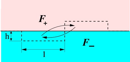
Figure 1: Interchange variation at the surface of gradient discontinuity.

3 Interchange driving force

While it is natural that condition (2.12) of strong local stability of the interface implies strong local stability of each individual deformation gradient $\bm{F}_{+}$ and $\bm{F}_{-}$, a less obvious claim of Theorem 2.2 is that the only joint stability constraint on the kinematically compatible pair $(\bm{F}_{+},\bm{F}_{-})$ is provided by condition ($I$). A natural challenge is then to identify the variation producing this condition.

We observe that conventional variations, linking both sides of a jump discontinuity and leading to Maxwell condition [8] or roughening instability condition [11], represent combinations of weak and strong variations. This creates unnecessary coupling and obscures the strong character of the minimizer under consideration. Physically it is clear that if ”materials” on both sides of the interface are stable and if we can interchange one ”material” by another without increasing the energy, then the whole configuration should be stable.

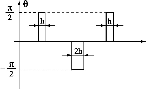
Figure 2: Strong double-dipole variation of the interface normal. The angle $\theta$ between the original and perturbed normals is plotted as a function of length in the tangential direction.

The idea of material interchange is illustrated schematically in Fig. 1 where the two adjacent rectangular domains are flipped and then translated. At $h\rightarrow 0$ this construction can be viewed as a interface generalization of the Weierstrass ”needle variation” since neither the fields are modified, except on a set of zero surface area. As we show in Fig. 2 this variation can be also interpreted as a strong variation of the interface normal.

Notice that if taken literally, the schematics of perturbed field shown in Fig. 1 is incompatible with a gradient of any admissible variation. To fix this technical problem we present below an explicit construction of the variation whose gradient differs significantly from the one shown in Fig. 1 only on a set of an infinitesimal measure.

We define a family of Lipschitz cut-off functions $\{\zeta_{h}(t):h\in(0,1)\}$ on $[0,+\infty)$ such that $\zeta_{h}(t)=1$, when $0\leq t\leq 1-\sqrt{h}$, while $\zeta_{h}(t)=0$, when $t\geq 1$. Let $\rho(t)$ be another Lipschitz cut-off function with $\rho(t)=1$, when $t>1$ and $\rho(t)=0$, when $t<0$. Suppose that $\bm{\eta}$ is a unit vector in $\mathbb{R}^{d}$, such that $\bm{\eta}\perp\bm{n}$. We then define the test function $\bm{\Phi}_{h}(\bm{z})$, to be used in (2.11), as follows

$$\bm{\Phi}_{h}=\bm{\Phi}_{h}^{+}+\bm{\Phi}_{h}^{-},\quad\bm{\Phi}_{h}^{-}(\bm{z})=\bm{\Phi}_{h}^{+}(-\bm{z}),\quad\bm{\Phi}^{+}_{h}(\bm{z})=h\phi\left(\frac{\bm{z}\cdot\bm{n}}{h}\right)\rho\left(\frac{\bm{z}\cdot\bm{\eta}}{\sqrt{h}}\right)\zeta_{h}(|\bm{z}|)\bm{a},$$ (3.1)

where

$$\phi(s)=\begin{cases}1-s,&0<s<1,\\ 1,&s\leq 0,\\ 0,&s\geq 1.\end{cases}$$

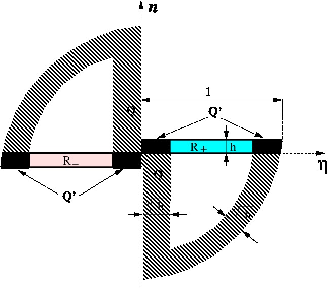
(a) Value map of $|\nabla\Phi_{h}|$ in the $(\bm{\eta},\bm{n})$-plane.

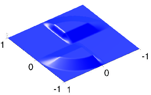
(b) Graph of $\Phi_{h}(\bm{z})$ over the $(\bm{\eta},\bm{n})$-plane.

Figure 3: Interchange variation $\bm{\Phi}_{h}(\bm{z})=\Phi_{h}(\bm{z})\bm{a}$.

Observe that $\bm{\Phi}_{h}(\bm{z})=\Phi_{h}(\bm{z})\bm{a}$, where the graph of $\Phi_{h}(\bm{z})$ is given in Figure 3(b). We remark that the variation (3.1) belongs to the class of multiscale variations proposed in [11]: it uses a small scale $h$ and another small scale $\epsilon$ from (2.5).

The interpretation of the function $\mathfrak{N}$ as an ”interchange driving force” is immediately clear from the following theorem:

Theorem 3.1.

Suppose $\{\bm{F}_{+},\bm{F}_{-}\}\subset\mathbb{M}$ satisfy (2.4). Let $\bm{\Phi}_{h}$ be given by (3.1). Then

$$\lim_{h\to 0}\displaystyle\frac{1}{h}\int_{B}\{W(\nabla\bar{\bm{y}}+\nabla\bm{\Phi}_{h}(\bm{z}))-W(\nabla\bar{\bm{y}})\}d\bm{z}=-\frac{\omega_{d-1}}{2}\mathfrak{N},$$ (3.2)

where $\bar{\bm{y}}(\bm{z})$ is given by (2.15) and $\omega_{k}=\pi^{k/2}/\Gamma(k/2+1)$ is the $k$ dimensional volume of the unit ball in $\mathbb{R}^{k}$.

Proof.

In order to compute the energy increment

$$\Delta E(h)=\int_{B}\{W(\nabla\bar{\bm{y}}+\nabla\bm{\Phi}_{h}(\bm{z}))-W(\nabla\bar{\bm{y}})\}d\bm{z}$$ (3.3)

we use the Weierstrass function

$$W^{\circ}(\bm{F},\bm{H})=W(\bm{F}+\bm{H})-W(\bm{F})-(W_{\bm{F}}(\bm{F}),\bm{H}).$$ (3.4)

We can then rewrite the energy increment $\Delta E(h)$ as

$$\Delta E(h)=\int_{B}W^{\circ}(\nabla\bar{\bm{y}},\nabla\bm{\Phi}_{h})d\bm{z}+\int_{B}(W_{\bm{F}}(\nabla\bar{\bm{y}}),\nabla\bm{\Phi}_{h})d\bm{z}.$$

We easily compute

$$\int_{B}(W_{\bm{F}}(\nabla\bar{\bm{y}}),\nabla\bm{\Phi}_{h})d\bm{z}=-\left([\![\bm{P}]\!]\bm{n},\int_{\Pi_{\bm{n}}\cap B}\bm{\Phi}_{h}dS\right)=-h\omega_{d-1}\mathfrak{N}+O(h^{3/2}).$$ (3.5)

Observe that $\bm{\Phi}^{+}_{h}(\bm{z})$ is non-zero only on $\bm{z}\cdot\bm{\eta}>0$, while $\bm{\Phi}^{-}_{h}(\bm{z})$ is non-zero only on $\bm{z}\cdot\bm{\eta}<0$. Therefore,

$$\int_{B}W^{\circ}(\nabla\bar{\bm{y}},\nabla\bm{\Phi}_{h})d\bm{z}=\int_{B}W^{\circ}(\nabla\bar{\bm{y}},\nabla\bm{\Phi}_{h}^{+})d\bm{z}+\int_{B}W^{\circ}(\nabla\bar{\bm{y}},\nabla\bm{\Phi}_{h}^{-})d\bm{z}.$$

In order to estimate the right-hand side, we identify 3 regions where $\nabla\bm{\Phi}_{h}\not=\bm{0}$ (see Figure 3(a)):

$$R_{\pm}=\{\bm{z}\in B:\pm\bm{z}\cdot\bm{\eta}>\sqrt{h},\ 0<\pm\bm{z}\cdot\bm{n}<h,\ |\bm{z}|<1-\sqrt{h}\},$$

$$Q=\{\bm{z}\in B:|\bm{z}|>1-\sqrt{h},\ (\bm{z}\cdot\bm{\eta})(\bm{z}\cdot\bm{n})<0\}\cup\\ \{\bm{z}\in B:|\bm{z}\cdot\bm{\eta}|<\sqrt{h},\ (\bm{z}\cdot\bm{\eta})(\bm{z}\cdot\bm{n})<0,\ |\bm{z}|<1-\sqrt{h}\},$$

and

$$Q^{\prime}=\{\bm{z}\in B:|\bm{z}\cdot\bm{\eta}|<\sqrt{h},\ |\bm{z}\cdot\bm{n}|<h,\ (\bm{z}\cdot\bm{\eta})(\bm{z}\cdot\bm{n})>0\}\cup\\ \{\bm{z}\in B:|\bm{z}|>1-\sqrt{h},\ |\bm{z}\cdot\bm{n}|<h,\ (\bm{z}\cdot\bm{\eta})(\bm{z}\cdot\bm{n})>0\}.$$

In order to estimate $\nabla\bm{\Phi}_{h}$ we write $\bm{\Phi}_{h}^{\pm}=\bm{\phi}_{h}^{\pm}c_{h}^{\pm}$, where

$$\bm{\phi}_{h}^{\pm}(\bm{z})=h\phi\left(\pm\frac{\bm{z}\cdot\bm{n}}{h}\right)\bm{a},\quad c_{h}^{\pm}(\bm{z})=\rho\left(\pm\frac{\bm{z}\cdot\bm{\eta}}{\sqrt{h}}\right)\zeta_{h}(|\bm{z}|).$$

It is easy to see that

$$|\bm{\phi}_{h}^{\pm}|=O(h),\quad|c_{h}^{\pm}|=O(1),\quad|\nabla\bm{\phi}_{h}^{\pm}|=O(1),\quad|\nabla c_{h}^{\pm}|=O\left(\displaystyle\frac{1}{\sqrt{h}}\right).$$

We see that $c_{h}^{\pm}=1$ and $\nabla\bm{\phi}^{\pm}_{h}=\mp[\![\bm{F}]\!]$ in regions $R_{\pm}$, $\bm{\phi}_{h}^{\pm}=h\bm{a}$ in the region $Q$. Thus

$$\nabla\bm{\Phi}_{h}^{\pm}(\bm{z})=\begin{cases}\mp[\![\bm{F}]\!],&\bm{z}\in R_{\pm},\\ h\bm{a}\otimes\nabla c_{h}^{\pm},&\bm{z}\in Q,\\ c_{h}^{\pm}\nabla\bm{\phi}_{h}^{\pm}+\bm{\phi}_{h}^{\pm}\otimes\nabla c_{h}^{\pm},&\bm{z}\in Q^{\prime},\\ \bm{0},&\text{elsewhere}.\end{cases}$$

Thus, $\nabla\bm{\Phi}_{h}=O(\sqrt{h})$ in the region $Q$ and $\nabla\bm{\Phi}_{h}=O(1)$ in region $Q^{\prime}$. We also see that $|Q|=O(\sqrt{h})$, $|Q^{\prime}|=O(h^{3/2})$, while $|R_{\pm}|=h\omega_{d-1}/2+O(h^{3/2})$. Thus, we estimate

$$\int_{Q\cup Q^{\prime}}W^{\circ}(\nabla\bar{\bm{y}},\nabla\bm{\Phi}_{h})d\bm{z}=O(h^{3/2}),$$

while

$$\int_{R_{\pm}}W^{\circ}(\nabla\bar{\bm{y}},\nabla\bm{\Phi}_{h}^{\pm})d\bm{z}=\frac{h\omega_{d-1}}{2}W^{\circ}(\bm{F}_{\pm},\mp[\![\bm{F}]\!])+O(h^{3/2}).$$

We conclude that

$$\lim_{h\to 0}\displaystyle\frac{1}{h}\int_{B}W^{\circ}(\nabla\bar{\bm{y}},\nabla\bm{\Phi}_{h})d\bm{z}=\frac{\omega_{d-1}}{2}\left(W^{\circ}(\bm{F}_{+},-[\![\bm{F}]\!])+W^{\circ}(\bm{F}_{-},[\![\bm{F}]\!])\right)=\frac{\omega_{d-1}}{2}\mathfrak{N}.$$ (3.6)

Combining (3.5) and (3.6) we obtain (3.2). ∎

While the Theorem 3.1 associates the interchange stability ($I$) with strong variations, the function $\mathfrak{N}$ is also known to be linked with stability with respect to weak variations. Indeed, after being projected onto the shear vector $\bm{a}$, the traction continuity condition $[\![\bm{P}]\!]\bm{n}=0$, which can be viewed as a weak form of Euler-Lagrange equations, gives the following normality condition [17]

$$\mathfrak{N}=([\![\bm{P}]\!],[\![\bm{F}]\!])=0.$$ (3.7)

To understand the origin of (3.7) consider the energy increment corresponding to classical weak variations

$$\bar{\bm{y}}\mapsto\bar{\bm{y}}(\bm{z})+\epsilon\bm{\phi}(\bm{z}),\qquad\bm{\phi}\in C_{0}^{1}(B;\mathbb{R}^{m}).$$ (3.8)

We obtain

$$\lim_{\epsilon\to 0}\displaystyle\frac{1}{\epsilon}\int_{B}\{W(\nabla\bar{\bm{y}}+\epsilon\nabla\bm{\phi})-W(\nabla\bar{\bm{y}})\}d\bm{z}=-\int_{\Pi_{\bm{n}}}([\![\bm{P}]\!]\bm{n},\bm{\phi})dS(\bm{z}).$$ (3.9)

The formula (3.9) shows that if $\bm{\phi}(\bm{z})=\bm{a}\phi(\bm{z})$ then the vanishing of the first variation implies the normality condition (3.7).

The crucial observation is that our strong variation $\bm{\Phi}_{h}$ given by (3.1) is also a scalar multiple of $\bm{a}$. This suggests the idea that our both weak and strong variations can be regarded as two limits of a single continuum of variations $\{t\bm{\Phi}_{h}:t\in[0,1]\}$ interpolating between them. Indeed, it is easy to see that if $t\to 0$ for fixed $h$, the two-parameter family of functions $t\bm{\Phi}_{h}$ converges to the weak variation (3.8), and when $h\to 0$ at $t=1$, we obtain the strong variation (3.1).

To compute the corresponding asymptotics of the energy increment we can use the method used in the proof of Theorem 3.1 which is applicable for any $t>0$. Let

$$\Delta E(t,h)=\int_{B}(W(\nabla\bar{\bm{y}}+t\nabla\bm{\Phi}_{h}(\bm{z}))-W(\nabla\bar{\bm{y}}))d\bm{z}.$$

Rewriting the energy increment in terms of the Weierstrass function we obtain

$$\Delta E(t,h)=\int_{B}W^{\circ}(\nabla\bar{\bm{y}},t\nabla\bm{\Phi}_{h})d\bm{z}+t\int_{B}(W_{\bm{F}}(\nabla\bar{\bm{y}}),\nabla\bm{\Phi}_{h})d\bm{z}.$$

Thus,

$$\lim_{t\to 0}\frac{\Delta E(t,h)}{t}=\int_{B}(W_{\bm{F}}(\nabla\bar{\bm{y}}),\nabla\bm{\Phi}_{h})d\bm{z}.$$

When $t>0$ is fixed we repeat the steps in the proof of Theorem 3.1 and obtain

$$\lim_{h\to 0}\displaystyle\frac{1}{h}\int_{B}W^{\circ}(\nabla\bar{\bm{y}},t\nabla\bm{\Phi}_{h})d\bm{z}=\frac{\omega_{d-1}}{2}(W^{\circ}(\bm{F}_{+},-t[\![\bm{F}]\!])+W^{\circ}(\bm{F}_{-},t[\![\bm{F}]\!])).$$

Hence, using the formula (3.5) we obtain

$$\lim_{h\to 0}\frac{\Delta E(t,h)}{h}=\frac{\omega_{d-1}}{2}(W^{\circ}(\bm{F}_{+},-t[\![\bm{F}]\!])+W^{\circ}(\bm{F}_{-},t[\![\bm{F}]\!])-2t\mathfrak{N}),$$ (3.10)

and

$$\lim_{h\to 0}\lim_{t\to 0}\frac{\Delta E(t,h)}{th}=-\omega_{d-1}\mathfrak{N}.$$

From (3.10) we obtain

$$\lim_{t\to 0}\lim_{h\to 0}\frac{\Delta E(t,h)}{th}=-\omega_{d-1}\mathfrak{N},$$

which shows that the $h$ and $t$ limits commute.

The existence of an explicit interpolation between weak and strong variations suggests to examine the behavior of the normalized energy along the connecting path. To this end, consider the expression

$$D(t)=\lim_{h\to 0}\frac{2\Delta E(t,h)}{h\omega_{d-1}}=W^{\circ}(\bm{F}_{+},-t[\![\bm{F}]\!])+W^{\circ}(\bm{F}_{-},t[\![\bm{F}]\!])-2t\mathfrak{N}$$

on the interval $[0,1]$. To ensure the symmetry of the two limits, we consider the special case $\mathfrak{N}=0$.

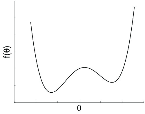
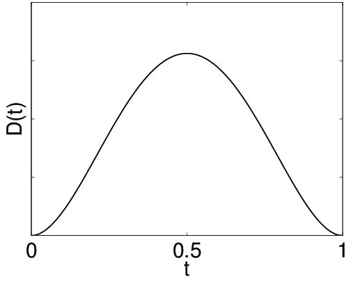
Figure 4: Connecting the weak ($t=0$) and the interchange ($t=1$) variation.

It is clear that the fine structure of the energy landscape along such a path is not universal and depends sensitively on the function $W(\bm{F})$. For the purpose of illustration, let us consider the energy density

$$W(\bm{F})=f(\theta)+\mu\left|\bm{\varepsilon}-\frac{\theta}{d}\bm{I}\right|^{2},\qquad\theta=\mathrm{Tr}\,\bm{F},\quad\bm{\varepsilon}=\frac{\bm{F}+\bm{F}^{T}}{2}.$$

Assuming kinematic compatibility (2.4) and normality (3.7) we obtain

$$D(t)=f(\theta_{t})+f(\widetilde{\theta}_{t})-f(\theta_{+})-f(\theta_{-})+t(1-t)[\![f^{\prime}(\theta)]\!][\![\theta]\!],$$

where

$$\theta_{t}=t\theta_{+}+(1-t)\theta_{-},\qquad\widetilde{\theta}_{t}=(1-t)\theta_{+}+t\theta_{-},$$

with $\theta_{\pm}$ satisfying

$$[\![\Phi^{\prime}]\!][\![\theta]\!]\leq 0,\qquad\Phi(\theta)=f(\theta)+\mu\left(1-\displaystyle\frac{1}{d}\right)\theta^{2}.$$

One can see that if the function $f(\theta)$ has a “double-well” structure (see Figure 4(a)) the graph of $D(t)$ looks like $t^{2}(1-t)^{2}$, see Figure 4(b). The presence of “energy barrier” indicates that any “combination” of the interchange variation and the weak variation (3.8) produces a cruder test of stability than either of the pure variations, incapable of detecting the existing instability. This result confirms our intuition that the realms of weak and strong variations are well separated and that the energy landscapes in the strong and weak topologies can be regarded as unrelated (unless all non-trivial features are removed by assuming uniform convexity or quasiconvexity).

We conclude this section by proving an important property of the interchange driving force $\mathfrak{N}$. More specifically, we show that if the deformation gradients $\bm{F}_{\pm}$ are strongly locally stable and if they are linked only by the kinematic compatibility condition (2.4), then the interchange driving force $\mathfrak{N}$ is non-negative.

We first recall the definition of the Maxwell driving force [7, 8]

$$p^{*}=[\![W]\!]-(\{{\{{\!\mkern-14.7mu}\mkern 14.7mu}{}\!\bm{P}\!\!{\}{\}\mkern 14.7mu}\mkern-14.7mu}{},[\![\bm{F}]\!]),$$ (3.11)

where $\{{\{{\!\mkern-14.7mu}\mkern 14.7mu}{}\!\bm{P}\!\!{\}{\}\mkern 14.7mu}\mkern-14.7mu}{}=\displaystyle\frac{1}{2}{(\bm{P}_{+}+\bm{P}_{-})}$.

Theorem 3.2.

Assume that both $\bm{F}_{+}$ and $\bm{F}_{-}$ are strongly locally stable and satisfy the kinematic compatibility condition (2.4). Then

$$\mathfrak{N}\geq 2|p^{*}|.$$ (3.12)

In particular, $\mathfrak{N}\geq 0$.

The theorem is an immediate consequence of Lemma 3.4 below, that shows that the algebraic inequality (3.12) is a consequence of the “Weierstrass condition” stated in the next lemma.

Lemma 3.3.

Suppose $\bm{F}$ is strongly locally stable. Then the Weierstrass condition holds

$$W^{\circ}(\bm{F},\bm{u}\otimes\bm{v})\geq 0,\text{ for all }\bm{u}\in\mathbb{R}^{m},\ \bm{v}\in\mathbb{R}^{d}.$$ (3.13)

The proof of the lemma can be found in [20, 13].

Lemma 3.4.

Suppose that both $\bm{F}_{+}$ and $\bm{F}_{-}$ satisfy the Weierstrass condition (3.13) and the kinematic compatibility condition (2.4). Then the inequality (3.12) holds.

Proof.

Setting $\bm{F}=\bm{F}_{\pm}$ and $\bm{u}\otimes\bm{v}=\mp[\![\bm{F}]\!]$ in (3.13), we obtain

$$W^{\circ}(\bm{F}_{\pm},\mp[\![\bm{F}]\!])=W(\bm{F}_{\mp})-W(\bm{F}_{\pm})\pm(\bm{P}_{\pm},[\![\bm{F}]\!])=\mp([\![W]\!]-(\bm{P}_{\pm},[\![\bm{F}]\!])).$$

Writing $\bm{P}_{\pm}=\{{\{{\!\mkern-14.7mu}\mkern 14.7mu}{}\!\bm{P}\!\!{\}{\}\mkern 14.7mu}\mkern-14.7mu}{}\pm\displaystyle\frac{1}{2}[\![\bm{P}]\!]$, where $\{{\{{\!\mkern-14.7mu}\mkern 14.7mu}{}\!\bm{P}\!\!{\}{\}\mkern 14.7mu}\mkern-14.7mu}{}=(\bm{P}_{+}+\bm{P}_{-})/2$, we obtain

$$W^{\circ}(\bm{F}_{\pm},\mp[\![\bm{F}]\!])=\mp p^{*}+\frac{\mathfrak{N}}{2}\geq 0.$$ (3.14)

The inequality (3.12) follows. ∎

Theorem  3.2, whose proof is now straightforward, quantifies to what extend conditions of stability of surfaces of jump discontinuity are stronger than conditions of strong local stability of each individual phase.

4 Proof of the main theorem

We are now in a position to prove Theorem 2.2. The necessity of (S) was already observed in Section 2, and the necessity of (I), even with equality, was shown in Section 3. The proof of sufficiency will be split into a sequence of lemmas. Our first step will be to recover the known interface jump conditions. In order to prove these algebraic relations only the Weierstrass condition (3.13) will be needed.

Lemma 4.1.

Assume that the pair $\bm{F}_{\pm}$ satisfies the following three conditions

• Kinematic compatibility: $[\![\bm{F}]\!]=\bm{a}\otimes\bm{n}$ for some $\bm{a}\in\mathbb{R}^{m}$ and $\bm{n}\in\mathbb{S}^{d-1}$,

• Interchange stability of the interface: $\mathfrak{N}=([\![\bm{P}]\!],[\![\bm{F}]\!])\leq 0$,

• Weierstrass condition: $W^{\circ}(\bm{F}_{\pm},\bm{u}\otimes\bm{v})\geq 0$ for all $\bm{u}\in\mathbb{R}^{m}$ and $\bm{v}\in\mathbb{R}^{d}$.

Then the following interface conditions must hold:

• The Maxwell jump condition

  $$p^{*}=0.$$ (4.1)

• Traction continuity

  $$[\![\bm{P}]\!]\bm{n}=\bm{0}.$$ (4.2)

• Interface roughening condition [11]

  $$[\![\bm{P}]\!]^{T}\bm{a}=\bm{0}.$$ (4.3)

Proof.

Combining Lemma 3.4 with (I) we conclude that $\mathfrak{N}=0$, and hence, by (3.12), the Maxwell condition (4.1) holds. In order to prove the remaining equalities we set $\bm{u}=\mp(\bm{a}+\bm{\xi})$ and $\bm{v}=\bm{n}+\bm{\eta}$ in the Weierstrass condition (W), where $\bm{a}$ and $\bm{n}$ are as in (2.4) and $\bm{\xi}$ and $\bm{\eta}$ are small parameters. Then we obtain a pair of inequalities

$$\omega_{\pm}(\bm{\xi},\bm{\eta})=W^{\circ}(\bm{F}_{\pm},\mp(\bm{a}+\bm{\xi})\otimes(\bm{n}+\bm{\eta}))\geq 0$$ (4.4)

that hold for all $\bm{\xi}\in\mathbb{R}^{m}$ and all $\bm{\eta}\in\mathbb{R}^{d}$. Under our smoothness assumptions on $W(\bm{F})$ the functions $\omega_{\pm}(\bm{\xi},\bm{\eta})$ are of class $C^{2}$ in the neighborhood of $(\bm{0},\bm{0})$ in the $(\bm{\xi},\bm{\eta})$-space. The Taylor expansion up to first order in $(\bm{\xi},\bm{\eta})$ gives

$$\omega_{\pm}(\bm{\xi},\bm{\eta})=\mp p^{*}+\frac{\mathfrak{N}}{2}+([\![\bm{P}]\!]\bm{n},\bm{\xi})+([\![\bm{P}]\!]^{T}\bm{a},\bm{\eta})+O(|\bm{\xi}|^{2}+|\bm{\eta}|^{2}).$$ (4.5)

Then the inequalities (4.4), together with $\mathfrak{N}=0$ and (4.1) imply (4.2) and (4.3). ∎

Next we prove a differentiability lemma that guarantees the existence of rank-1 directional derivatives of quasiconvex and rank-1 convex envelopes at “marginally stable” deformation gradients [12]. This result does not require any additional growth conditions, as in the envelope regularity theorems from [3].

Lemma 4.2.

Let $V(\bm{F})$ be a rank-one convex function such that $V(\bm{F})\leq W(\bm{F})$. Let

$${\mathcal{A}}_{V}=\{\bm{F}\in{\mathcal{O}}:W(\bm{F})=V(\bm{F})\},$$

where ${\mathcal{O}}$ is an open subset of $\mathbb{M}$ on which $W(\bm{F})$ is of class $C^{1}$. Then for every $\bm{F}\in{\mathcal{A}}_{V}$ and every $\bm{u}\in\mathbb{R}^{m}$, $\bm{v}\in\mathbb{R}^{d}$

$$\lim_{t\to 0}\frac{V(\bm{F}+t\bm{u}\otimes\bm{v})-V(\bm{F})}{t}=(W_{\bm{F}}(\bm{F}),\bm{u}\otimes\bm{v}).$$ (4.6)

In particular,

$$V(\bm{F}+\bm{u}\otimes\bm{v})\geq W(\bm{F})+(W_{\bm{F}}(\bm{F}),\bm{u}\otimes\bm{v}).$$

Proof.

By our assumption $v(t)=V(\bm{F}+t\bm{u}\otimes\bm{v})$ is convex on $\mathbb{R}$. Recall from the theory of convex functions that

$$q(t)=\frac{v(t)-v(0)}{t}$$

is monotone increasing on each of the intervals $(-\infty,0)$, $(0,+\infty)$. Therefore, the limits

$$v^{\prime}(0^{\pm})=\lim_{t\to 0^{\pm}}\frac{v(t)-v(0)}{t}$$

exist. Moreover, the convexity of $v(t)$ implies that $v^{\prime}(0^{-})\leq v^{\prime}(0^{+})$. Let $w(t)=W(\bm{F}+t\bm{u}\otimes\bm{v})$. By assumption $v(t)\leq w(t)$. We also have $v(0)=w(0)$, since $\bm{F}\in{\mathcal{A}}_{V}$. When $t>0$

$$\frac{v(t)-v(0)}{t}\leq\frac{w(t)-w(0)}{t}.$$

Therefore, $v^{\prime}(0^{+})\leq w^{\prime}(0)$. Similarly, when $t<0$ we obtain $v^{\prime}(0^{-})\geq w^{\prime}(0)$. Thus,

$$w^{\prime}(0)\leq v^{\prime}(0^{-})\leq v^{\prime}(0^{+})\leq w^{\prime}(0).$$

We conclude that the limit on the left-hand side of (4.6) exists and is equal to

$$w^{\prime}(0)=(W_{\bm{F}}(\bm{F}),\bm{u}\otimes\bm{v}).$$

Thus, the convex function $v(t)$ is differentiable at $t=0$ and $v=w(0)+w^{\prime}(0)t$ is a tangent line to its graph at $t=0$. Convexity of $v(t)$ then implies that $v(t)\geq w(0)+w^{\prime}(0)t$ for all $t\in\mathbb{R}$. ∎

In general, one does not expect explicit formulas for the values of the quasiconvex envelope $QW$ in terms of $W$. In that respect Lemma 4.3 below provides a nice exception to the rule.

Lemma 4.3.

Assume that the pair $\bm{F}_{\pm}$ satisfies all conditions of Theorem 2.2. Then

$$QW(t\bm{F}_{+}+(1-t)\bm{F}_{-})=RW(t\bm{F}_{+}+(1-t)\bm{F}_{-})=tW(\bm{F}_{+})+(1-t)W(\bm{F}_{-})$$ (4.7)

for all $t\in[0,1]$, where $RW(\bm{F})$ is the rank-1 convex envelope of $W(\bm{F})$ [6].

Proof.

By assumption (S) we have $QW(\bm{F}_{\pm})=W(\bm{F}_{\pm})\geq RW(\bm{F}_{\pm})\geq QW(\bm{F}_{\pm})$. Therefore,

$$QW(\bm{F}_{\pm})=W(\bm{F}_{\pm})=RW(\bm{F}_{\pm}).$$ (4.8)

By rank-one convexity of $QW(\bm{F})$ [22, 1, 6] and assumptions (K) and (S) we have

$$QW(t\bm{F}_{+}+(1-t)\bm{F}_{-})\leq tQW(\bm{F}_{+})+(1-t)QW(\bm{F}_{-})=tW(\bm{F}_{+})+(1-t)W(\bm{F}_{-}).$$ (4.9)

To prove the opposite inequality we apply Lemma 4.2 and obtain

$$QW(t\bm{F}_{+}+(1-t)\bm{F}_{-})\geq W(\bm{F}_{-})+(\bm{P}_{-},t[\![\bm{F}]\!])=tW(\bm{F}_{+})+(1-t)W(\bm{F}_{-})-tp^{*}-\frac{t}{2}\mathfrak{N}.$$ (4.10)

Thus, Lemma 4.1, (4.9) and (4.10) result in the formula for $QW(t\bm{F}_{+}+(1-t)\bm{F}_{-})$ from (4.7). We also have, in view of the assumption (K) and (4.8), that

$$tW(\bm{F}_{+})+(1-t)W(\bm{F}_{-})=QW(t\bm{F}_{+}+(1-t)\bm{F}_{-})\leq RW(t\bm{F}_{+}+(1-t)\bm{F}_{-})\leq\\ tRW(\bm{F}_{+})+(1-t)RW(\bm{F}_{-})=tW(\bm{F}_{+})+(1-t)W(\bm{F}_{-}).$$

Formula (4.7) is now proved. ∎

We are now ready to establish the inequality (2.12), proving Theorem 2.2. Let $\bm{\phi}_{0}\in W_{0}^{1,\infty}(B;\mathbb{R}^{m})$ be an arbitrary test function. Let $Q_{\bm{n}}$ be the cube with side 2 centered at the origin and having a face with normal $\bm{n}$. Consider a $Q_{\bm{n}}$-periodic function $\bar{\bm{F}}_{\rm per}(\bm{z})$ on $\mathbb{R}^{d}$ given on its period $Q_{\bm{n}}$ by

$$\bar{\bm{F}}_{\rm per}(\bm{z})=\left\{\begin{array}[]{ll}\bm{F}_{+},&\text{ if }\bm{z}\cdot\bm{n}>0\\ \bm{F}_{-},&\text{ if }\bm{z}\cdot\bm{n}<0.\end{array}\right.$$

Assumption (K) implies that

$$\bar{\bm{F}}_{\rm per}(\bm{z})=\{{\{{\!\mkern-14.7mu}\mkern 14.7mu}{}\!\bm{F}\!\!{\}{\}\mkern 14.7mu}\mkern-14.7mu}{}+\nabla(\psi(\bm{z}\cdot\bm{n})\bm{a}),\qquad\{{\{{\!\mkern-14.7mu}\mkern 14.7mu}{}\!\bm{F}\!\!{\}{\}\mkern 14.7mu}\mkern-14.7mu}{}=\displaystyle\frac{1}{2}(\bm{F}_{+}+\bm{F}_{-}),$$

where $\psi(\zeta)$ is a 2-periodic saw-tooth function such that that $\psi(\zeta)=|\zeta|/2$, $\zeta\in[-1,1]$. Let $\bm{\phi}_{\rm per}(\bm{z})$ be $Q_{\bm{n}}$-periodic function such that

$$\bm{\phi}_{\rm per}(\bm{z})=\begin{cases}\bm{\phi}_{0}(\bm{z}),&\bm{z}\in B,\\ \bm{0},&\bm{z}\in Q_{\bm{n}}\setminus B.\end{cases}$$

This function is Lipschitz continuous, since $\bm{\phi}_{0}\in W_{0}^{1,\infty}(B;\mathbb{R}^{m})$ and $B\subset Q_{\bm{n}}$. The function $QW(\bm{F})$ is quasiconvex and the function $\bm{\phi}_{\rm per}(\bm{z})+\psi(\bm{z}\cdot\bm{n})\bm{a}$ is $Q_{\bm{n}}$-periodic. Therefore (see [6]),

$$QW(\{{\{{\!\mkern-14.7mu}\mkern 14.7mu}{}\!\bm{F}\!\!{\}{\}\mkern 14.7mu}\mkern-14.7mu}{})\leq\mathchoice{{\vbox{\hbox{$\textstyle-$ }}\kern-7.83337pt}}{{\vbox{\hbox{$\scriptstyle-$ }}\kern-5.90005pt}}{{\vbox{\hbox{$\scriptscriptstyle-$ }}\kern-4.75003pt}}{{\vbox{\hbox{$\scriptscriptstyle-$ }}\kern-4.25003pt}}\!\int_{Q_{\bm{n}}}QW(\{{\{{\!\mkern-14.7mu}\mkern 14.7mu}{}\!\bm{F}\!\!{\}{\}\mkern 14.7mu}\mkern-14.7mu}{}+\nabla(\bm{\phi}_{\rm per}+\psi(\bm{z}\cdot\bm{n})\bm{a}))d\bm{z}\leq\mathchoice{{\vbox{\hbox{$\textstyle-$ }}\kern-7.83337pt}}{{\vbox{\hbox{$\scriptstyle-$ }}\kern-5.90005pt}}{{\vbox{\hbox{$\scriptscriptstyle-$ }}\kern-4.75003pt}}{{\vbox{\hbox{$\scriptscriptstyle-$ }}\kern-4.25003pt}}\!\int_{Q_{\bm{n}}}W(\bar{\bm{F}}_{\rm per}(\bm{z})+\nabla\bm{\phi}_{\rm per})d\bm{z}.$$

By Lemma 4.3

$$QW(\{{\{{\!\mkern-14.7mu}\mkern 14.7mu}{}\!\bm{F}\!\!{\}{\}\mkern 14.7mu}\mkern-14.7mu}{})=\{{\{{\!\mkern-14.7mu}\mkern 14.7mu}{}\!W\!\!{\}{\}\mkern 14.7mu}\mkern-14.7mu}{}=\mathchoice{{\vbox{\hbox{$\textstyle-$ }}\kern-7.83337pt}}{{\vbox{\hbox{$\scriptstyle-$ }}\kern-5.90005pt}}{{\vbox{\hbox{$\scriptscriptstyle-$ }}\kern-4.75003pt}}{{\vbox{\hbox{$\scriptscriptstyle-$ }}\kern-4.25003pt}}\!\int_{Q_{\bm{n}}}W(\bar{\bm{F}}_{\rm per}(\bm{z}))d\bm{z}.$$

Hence

$$\int_{Q_{\bm{n}}}W(\bar{\bm{F}}_{\rm per}(\bm{z}))d\bm{z}\leq\int_{Q_{\bm{n}}}W(\bar{\bm{F}}_{\rm per}(\bm{z})+\nabla\bm{\phi}_{\rm per})d\bm{z}.$$

The inequality (2.12) is proved, since $\bm{\phi}_{0}(\bm{z})$ is supported on $B$.

We remark that Theorem 2.2 answers the question studied in [25] by giving a complete characterization of all possible pairs of deformation gradient values $\bm{F}_{\pm}$ that can occur on a stable phase boundary. Global minimality of $\bar{\bm{y}}(\bm{z})$, given by (2.15) also implies that any other interface conditions, like, for example, local Grinfeld condition [10] or roughening stability inequality [11, Remark 4.2], must be consequences of (K), (I) and (S).

5 An example of strongly locally stable interfaces

In this section we establish a relation between particular solutions of the variational problems (2.13) and (2.14) which elucidates the role played in the theory by the normality condition.

Consider the set $\mathfrak{B}$ of all $\bm{F}\in\mathbb{M}$ that are not strongly locally stable; we called this set the ”elastic binodal” in [12]. For such $\bm{F}$ the infimum in the variational problem (2.13) may be reachable only by minimizing sequences characterized by their Young measures [26, 18]. Suppose that for some $\bm{F}\in\mathfrak{B}$ the Young measure solution of (2.13) has the form of a simple laminate [23]:

$$\nu=\theta\delta_{\bm{F}_{+}}+(1-\theta)\delta_{\bm{F}_{-}},\qquad\bm{F}=\theta\bm{F}_{+}+(1-\theta)\bm{F}_{-},\quad 0<\theta<1.$$ (5.1)

The set $\mathfrak{B}_{1}$ of all such $\bm{F}\in\mathfrak{B}$ will be called the simple laminate region. There is a direct connection between the simple laminate region $\mathfrak{B}_{1}$ and locally stable interfaces.

Theorem 5.1.

A strongly locally stable interface determined by $\bm{F}_{\pm}$ corresponds to a straight line segment $\{\theta\bm{F}_{+}+(1-\theta)\bm{F}_{-}:\theta\in(0,1)\}\subset\mathfrak{B}_{1}$, so that the laminate Young measure (5.1) solves (2.13) with $\bm{F}=\theta\bm{F}_{+}+(1-\theta)\bm{F}_{-}$. Conversely, every point $\bm{F}\in\mathfrak{B}_{1}$, corresponding to a laminate Young measure (5.1) determines a strongly locally stable interface.

Proof.

If $\Pi_{\bm{n}}=\{\bm{z}\in\mathbb{R}^{d}:\bm{z}\cdot\bm{n}=0\}$ is a strongly locally stable interface determined by $\bm{F}_{+}$ and $\bm{F}_{-}$ then the pair $\bm{F}_{\pm}$ satisfies conditions (K), (I) and (S). By Lemma 4.3 the gradient Young measure (5.1) attains the minimum in (2.13) for $\bm{F}=\theta\bm{F}_{+}+(1-\theta)\bm{F}_{-}$, $\theta\in(0,1)$, and thus $\bm{F}\in\mathfrak{B}_{1}$. If $\mathfrak{B}_{1}$ has a non-empty interior then formula (4.7) says that the graph of the quasiconvex envelope $QW(\bm{F})$ over $\mathfrak{B}_{1}$ is formed by straight line segments joining $(\bm{F}_{+},W(\bm{F}_{+}))$ and $(\bm{F}_{-},W(\bm{F}_{-}))$. In other words the graph of $QW(\bm{F})$ is a ruled surface.

Conversely, if the gradient Young measure (5.1) attains the minimum in (2.13), then $\bm{F}_{\pm}$ satisfy the kinematic compatibility condition (2.4) and

$$QW(\theta\bm{F}_{+}+(1-\theta)\bm{F}_{-})=\theta W(\bm{F}_{+})+(1-\theta)W(\bm{F}_{-}).$$ (5.2)

The difference between (5.2) and (4.7) is that (5.2) is assumed to hold for a single fixed value of $\theta\in(0,1)$. Therefore, both material stability (S) at $\bm{F}_{\pm}$ and interchange stability (I) need to be established.

Lemma 5.2.

Assume that the pair $\bm{F}_{\pm}$ satisfies (2.4) and that (5.2) holds for some $\theta\in(0,1)$. Then $QW(\bm{F}_{\pm})=W(\bm{F}_{\pm})$ and $\mathfrak{N}=0$.

Proof.

The proof is based on the following general property of convex functions.

Lemma 5.3.

Let $\phi(t)$ be a convex function on $[0,1]$. Suppose that $\phi(\theta)=\theta\phi(1)+(1-\theta)\phi(0)$ for some $\theta\in(0,1)$. Then

$$\phi(t)=t\phi(1)+(1-t)\phi(0)$$ (5.3)

for all $t\in[0,1]$.

Proof.

By convexity

$$\phi(t)\leq t\phi(1)+(1-t)\phi(0),\quad t\in[0,1].$$ (5.4)

If $t\in(0,\theta)$, then

$$\theta=\lambda+(1-\lambda)t,\qquad\lambda=\frac{\theta-t}{1-t}\in(0,1).$$

Therefore, by the assumption of the lemma and convexity of $\phi$

$$\theta\phi(1)+(1-\theta)\phi(0)=\phi(\theta)\leq\lambda\phi(1)+(1-\lambda)\phi(t).$$

It follows that

$$\phi(t)\geq\frac{(\theta-\lambda)\phi(1)+(1-\theta)\phi(0)}{1-\lambda}=t\phi(1)+(1-t)\phi(0).$$

This inequality in combination with (5.4) establishes (5.3) for $t\in(0,\theta)$. The proof of (5.3) for $t\in(\theta,1)$ is similar. ∎

To prove Lemma 5.2 we recall that $QW(\bm{F})\leq W(\bm{F})$ for all $\bm{F}\in\mathbb{M}$. By (5.2) and rank-1 convexity of $QW(\bm{F})$ we have

$$\theta W(\bm{F}_{+})+(1-\theta)W(\bm{F}_{-})=QW(\theta\bm{F}_{+}+(1-\theta)\bm{F}_{-})\leq\\ \theta QW(\bm{F}_{+})+(1-\theta)QW(\bm{F}_{-})\leq\theta W(\bm{F}_{+})+(1-\theta)W(\bm{F}_{-}),$$

which is possible if and only if $QW(\bm{F}_{\pm})=W(\bm{F}_{\pm})$. Then, defining

$$\phi(t)=QW(t\bm{F}_{+}+(1-t)\bm{F}_{-})$$

and applying Lemma 5.3 we obtain (4.7). We can also apply Lemma 4.2 with $\bm{F}=\bm{F}_{\pm}$, $V(\bm{F})=QW(\bm{F})$. The formula (4.6) allows us to differentiate (4.7) at $t=0$ and $t=1$:

$$(\bm{P}_{-},[\![\bm{F}]\!])=[\![W]\!],\qquad(\bm{P}_{+},[\![\bm{F}]\!])=[\![W]\!].$$

Subtracting the two equalities we obtain $\mathfrak{N}=0$. ∎

Thus, we have shown that every $\bm{F}$ in the simple laminate region $\mathfrak{B}_{1}$ gives rise to the pair $\bm{F}_{\pm}$ satisfying all conditions of Theorem 2.2. Theorem 2.2 then implies that the interface $\Pi_{\bm{n}}$ determined by $\bm{F}_{\pm}$ is strongly locally stable. Theorem 5.1 is now proved. ∎

Remark 5.4.

The system of algebraic equations (2.4), (4.1), (4.2) and (4.3) defines a co-dimension 1 surface $\mathfrak{J}\subset\mathbb{M}$ called the “jump set”. We have shown in [11] that under some non-degeneracy assumptions the jump set must lie in the closure of the binodal region $\mathfrak{B}$. In fact all points on the jump set are “marginally stable” and detectable through the nucleation of an infinite layer in an infinite space [12]. It follows that the existence of a strongly locally stable interface has significant consequences for the geometry of $\mathfrak{B}$. The presence of stable interfaces implies that a part of the jump set must coincide with a part of the “binodal”, the boundary of $\mathfrak{B}$. The rank-1 lines joining $\bm{F}_{+}$ and $\bm{F}_{-}$, both of which lie on the binodal, cover the simple lamination region $\mathfrak{B}_{1}\subset\mathfrak{B}$.

6 Analogy with plasticity theory

In this section we show that the algebraic equation

$$\mathfrak{N}=0,$$

interpreted above as condition of interchange equilibrium, is conceptually similar to the well known normality condition in plasticity theory [19, 9].

To build a link between the two frameworks we now show that a microstructure in elasticity theory plays the role of a “ mechanism” in plasticity theory. Consider a loading program with affine Dirichlet boundary conditions $\bm{y}(\bm{x})=\bm{F}(t)\bm{x}$. Suppose that $\bm{F}(t)\in\mathfrak{B}_{1}$ for an interval of values of the loading parameter $t$. Then, for every $t$ the deformation gradient $\bm{F}(t)$ will be accommodated by a laminate (5.1), so that

$$\bm{F}(t)=\theta(t)\bm{F}_{+}(t)+(1-\theta(t))\bm{F}_{-}(t).$$ (6.1)

We now interpret the representation (6.1) from the point of view of plasticity theory. While the deformations associated with the change of $\bm{F}_{+}$ and $\bm{F}_{-}$ in each layer of the laminate are elastic, the deformation associated with the change of parameter $t$, affecting the microstructure and modifying the Young measure $\nu$, can be regarded as “inelastic”. In fact, it is similar to lattice invariant shear characterizing elementary slip in crystal plasticity theory. To be more specific, we can decompose the strain rate $\dot{\bm{F}}$ as follows

$$\dot{\bm{F}}=\theta\dot{\bm{F}}_{+}+(1-\theta)\dot{\bm{F}}_{-}+\dot{\theta}[\![\bm{F}]\!]=\dot{\bm{\varepsilon}}^{e}+\dot{\bm{\varepsilon}}^{p},$$

where $\dot{\bm{\varepsilon}}^{e}=\theta\dot{\bm{F}}_{+}+(1-\theta)\dot{\bm{F}}_{-}$ is the elastic strain rate and $\dot{\bm{\varepsilon}}^{p}=\dot{\theta}[\![\bm{F}]\!]$ is the “plastic” strain rate.

Next we notice that in equilibrium the “inelastic” strain rate $\dot{\bm{\varepsilon}}^{p}$ defines an affine direction along the quasiconvex envelope of the energy (see Lemma 4.3). This suggests that there is a stress plateau with which one can associate a notion of the “yield” stress [19].

To find an equation for the corresponding “yield surface” we choose a special loading path where the elastic fields in the layers do not change $\dot{\bm{F}}_{\pm}=\bm{0}$. Then, differentiating (4.7) in $t$, we find that the total stress field $\bm{P}_{\rm tot}(t)=QW_{\bm{F}}(\bm{F}(t))$ lies on the hyperplane

$$\mathfrak{Y}_{{\mathcal{M}}}=\{\bm{P}:(\bm{P},[\![\bm{F}]\!])=[\![W]\!]\}$$ (6.2)

which we interpret as the “yield surface” associated with “plastic” mechanism ${\mathcal{M}}=(\bm{F}_{+},\bm{F}_{-})$. If we now rewrite our elastic normality condition $\mathfrak{N}=0$ in the form

$$(\bm{P}_{+},[\![\bm{F}]\!])=(\bm{P}_{-},[\![\bm{F}]\!]).$$ (6.3)

it becomes apparent that the “plastic” strain rate $\dot{\bm{\varepsilon}}^{p}=\dot{\theta}[\![\bm{F}]\!]$ is orthogonal to the yield surface $\mathfrak{Y}_{{\mathcal{M}}}$.

To strengthen the analogy we observe that in plasticity theory the yield surface marks the set of minimally stable elastic states [24]. In elastic framework the states $\bm{F}_{\pm}$ adjacent to the jump discontinuity are also only marginally stable, see Remark 5.4. The fact that in elasticity setting the normality condition appears as a part of energy minimization while in plasticity theory it is usually derived by maximizing plastic dissipation, is secondary in view of the implied rate independent nature of plastic dissipation [21].

The analogy between elastic and plastic normality conditions becomes more transparent if we consider a simple example. Suppose that our material is isotropic and the deformation is anti-plane shear. Take the energy density in the form

$$W(\bm{F})=\min\left\{\frac{\mu_{+}}{2}|\bm{F}|^{2}+w_{+},\frac{\mu_{-}}{2}|\bm{F}|^{2}+w_{-}\right\}.$$ (6.4)

where $\bm{F}\in\mathbb{R}^{2}$and the shear moduli of the “phases” $\mu_{\pm}$ are positive.

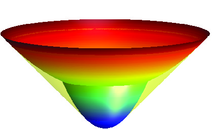
Figure 5: Anti-plane shear energy density function and its convex envelope.

In this scalar example the quasiconvex and convex envelopes of the energy density coincide, and hence we can write (see Fig. 5)

$$QW(\bm{F})=CW(\bm{F})=\left\{\begin{array}[]{ll}\dfrac{\mu_{+}}{2}|\bm{F}|^{2}+w_{+},&\text{ if }|\bm{F}|\leq\varepsilon_{+}\\[12.91663pt] \dfrac{\mu_{-}}{2}|\bm{F}|^{2}+w_{-},&\text{ if }|\bm{F}|\geq\varepsilon_{-}\\[12.91663pt] |\bm{F}|\sqrt{-\dfrac{2[\![w]\!]\mu_{+}\mu_{-}}{[\![\mu]\!]}}+\dfrac{[\![\mu w]\!]}{[\![\mu]\!]},&\text{ if }\varepsilon_{+}\leq|\bm{F}|\leq\varepsilon_{-}.\end{array}\right.,$$

where

$$\varepsilon_{+}=\sqrt{\dfrac{-2[\![w]\!]\mu_{-}}{[\![\mu]\!]\mu_{+}}},\qquad\varepsilon_{-}=\sqrt{-\dfrac{2[\![w]\!]\mu_{+}}{[\![\mu]\!]\mu_{-}}}.$$

Observe also that the binodal region

$$\mathfrak{B}=\{\bm{F}\in\mathbb{R}^{2}:\varepsilon_{+}\leq|\bm{F}|\leq\varepsilon_{-}\}.$$

coincides with the simple laminate region $\mathfrak{B}_{1}$ since for $\bm{F}_{0}\in\mathfrak{B}$ the gradient Young measures

$$\nu(\bm{F})=\theta\delta_{\bm{F}_{+}}(\bm{F})+(1-\theta)\delta_{\bm{F}_{-}}(\bm{F}),\qquad\theta=\frac{|\bm{F}_{0}|-\varepsilon_{-}}{[\![\varepsilon]\!]},\quad\bm{F}_{\pm}=\frac{\varepsilon_{\pm}}{|\bm{F}_{0}|}\bm{F}_{0}$$

attain the infimum in (2.13).

Figure 6: Envelope of yield lines in anti-plane shear.

By fixing $\bm{F}_{+}$ on the circle ${\mathcal{C}}_{+}=\{\bm{F}\in\mathbb{R}^{2}:|\bm{F}|=\varepsilon_{+}\}$ we then obtain the unique

$$\bm{F}_{-}=\frac{\varepsilon_{-}}{\varepsilon_{+}}\bm{F}_{+},$$

which furnishes the “plastic” mechanism ${\mathcal{M}}=(\bm{F}_{+},\bm{F}_{-})$. The associated “yield plane” $\mathfrak{Y}_{{\mathcal{M}}}$ can be written explicitly

$$\mathfrak{Y}_{{\mathcal{M}}}=\left\{\bm{P}\in\mathbb{R}^{2}:\bm{P}\cdot\bm{F}_{+}=\frac{2\varepsilon_{+}[\![w]\!]}{[\![\varepsilon]\!]}\right\}.$$

We observe that as $\bm{F}_{+}$ is varied over the circle ${\mathcal{C}}_{+}$, the yield lines $\mathfrak{Y}_{{\mathcal{M}}}$ form an envelope of the circle

$${\mathcal{P}}=\left\{\bm{P}\in\mathbb{R}^{2}:|\bm{P}|=\frac{2[\![w]\!]}{[\![\varepsilon]\!]}\right\},$$

in stress space (see Fig. 6), which is the image of the binodal $\partial\mathfrak{B}$ under the map $W_{\bm{F}}(\bm{F})$.

Since the stress in each phase of the laminate is always the same

$$\bm{P}_{+}=\bm{P}_{-}=\mu_{+}\bm{F}_{+}=\mu_{-}\bm{F}_{-},$$

we can write

$$|\bm{P}_{\pm}|^{2}=\mu_{+}^{2}\varepsilon_{+}^{2}=-\frac{2[\![w]\!]\mu_{+}\mu_{-}}{[\![\mu]\!]}=\frac{4[\![w]\!]^{2}}{[\![\varepsilon]\!]^{2}}.$$

Thus, in an arbitrary loading program the total stress $\bm{P}(t)=\theta\bm{P}_{+}+(1-\theta)\bm{P}_{-}$ will be confined to the yield surface envelope ${\mathcal{P}}$, provided $\bm{F}(t)\in\mathfrak{B}$.

Two cautionary notes are in order. First, in contrast with conventional plasticity theory, the regions of stress space both inside and outside of the “yield” surface ${\mathcal{P}}$ are elastic. This distinguishes our ”transformational plasticity” where hysteresis is infinitely narrow, from the classical plasticity where hysteresis is essential. Such geometric picture continue to hold as long as $[\![\bm{P}]\!]=\bm{0}$, in particular, it holds for all scalar problems ($m=1$). The second observation is that for $[\![\bm{P}]\!]\not=0$, our “hardening free” plastic analogy breaks down because the total stress in an arbitrary loading program is no longer confined to any surface. In this case the ”plastic” mechanism operates on a set of full measure and the proposed analogy requires a generalization.

7 Acknowledgement

This material is based upon work supported by the National Science Foundation under Grant No. 1008092 and the French ANR grant EVOCRIT (2008-2012).

References

[1]
J. M. Ball.
Convexity conditions and existence theorems in nonlinear elasticity.
Arch. Ration. Mech. Anal., 63(4):337–403, 1976/77.
[2]
J. M. Ball.
Some open problems in elasticity.
In Geometry, mechanics, and dynamics, pages 3–59. Springer,
New York, 2002.
[3]
J. M. Ball, B. Kirchheim, and J. Kristensen.
Regularity of quasiconvex envelopes.
Calc. Var. Partial Differential Equations, 11(4):333–359,
2000.
[4]
J. M. Ball and J. E. Marsden.
Quasiconvexity at the boundary, positivity of the second variation
and elastic stability.
Arch. Ration. Mech. Anal., 86(3):251–277, 1984.
[5]
B. Dacorogna.
Quasiconvexity and relaxation of nonconvex problems in the calculus
of variations.
J. Funct. Anal., 46(1):102–118, 1982.
[6]
B. Dacorogna.
Direct methods in the calculus of variations.
Springer-Verlag, New York, 1989.
[7]
G. Erdmann.
Über die unstetige Lösungen in der Variationsrechnung.
J. Reine Angew. Math., 82:21–30, 1877.
[8]
J. D. Eshelby.
Energy relations and energy momentum tensor in continuum mechanics.
In M. Kanninen, W. Adler, A. Rosenfeld, and R. Jaffee, editors, Inelastic behavior of solids, pages 77–114. McGraw-Hill, New York, 1970.
[9]
R. Fosdick and E. Volkmann.
Normality and convexity of the yield surface in nonlinear plasticity.
Quart. Appl. Math., 51:117–127, 1993.
[10]
Y. Grabovsky, V. A. Kucher, and L. Truskinovsky.
Weak variations of lipschitz graphs and stability of phase
boundaries.
Continuum Mechanics and Thermodynamics, in press, 2010.
[11]
Y. Grabovsky and L. Truskinovsky.
Roughening instability of broken extremals.
Arch. Rat. Mech. Anal., 200(1):183–202, 2011.
[12]
Y. Grabovsky and L. Truskinovsky.
Marginal material stability.
Journal of Nonlinear Science, 23(5):891–969, 2013.
[13]
L. M. Graves.
The weierstrass condition for multiple integral variation problems.
Duke Math. J., 5(3):656–660, 1939.
[14]
M. A. Grinfeld.
Stability of heterogeneous equilibrium in systems containing solid
elastic phases.
Dokl. Akad. Nauk SSSR, 265(4):836–840, 1982.
[15]
M. E. Gurtin.
Two-phase deformations of elastic solids.
Arch. Ration. Mech. Anal., 84(1):1–29, 1983.
[16]
J. Hadamard.
Mémoire sur le problème d’analyse relatif à
l’équilibre des plaques élastiques encastrées, volume 33 of
Mem. Acad. Sci. Paris.
Imprimerie nationale, 1908.
[17]
R. Hill.
Energy momentum tensors in elastostatics:some reflections on the
general theory.
J. Mech. Phys. Solids, 34:305–317, 1986.
[18]
D. Kinderlehrer and P. Pedregal.
Characterizations of Young measures generated by gradients.
Arch. Ration. Mech. Anal., 115(4):329–365, 1991.
[19]
J. Lubliner.
Plasticity theory.
Macmillan Publishing Company, New York, 1990.
[20]
E. J. McShane.
On the necessary condition of weierstrass in the multiple integral
problem of the calculus of variations.
Annals of Mathematics, 32(3):pp. 578–590, 1931.
[21]
A. Mielke and L. Truskinovsky.
From discrete visco-elasticity to continuum rate-independent
plasticity: rigorous results.
Archive for Rational Mechanics and Analysis, 203(2):577–619,
2012.
[22]
J. Morrey, Charles B.
Multiple integrals in the calculus of variations.
Springer-Verlag New York, Inc., New York, 1966.
Die Grundlehren der mathematischen Wissenschaften, Band 130.
[23]
P. Pedregal.
Laminates and microstructure.
European Journal of Applied Mathematics, 4:121–149, 6 1993.
[24]
O. Salman and L. Truskinovsky.
On the critical nature of plastic flow: One and two dimensional
models.
International Journal of Engineering Science, 59:219–254,
2012.
[25]
M. Šilhavý.
Maxwell’s relation for isotropic bodies.
In Mechanics of material forces, volume 11 of Adv. Mech.
Math., pages 281–288. Springer, New York, 2005.
[26]
L. Tartar.
Étude des oscillations dans les équations aux dérivées
partielles non linéaires.
In Trends and applications of pure mathematics to mechanics
(Palaiseau, 1983), pages 384–412. Springer-Verlag, Berlin, 1984.