Robust $T$-optimal discriminating designs

Abstract

This paper considers the problem of constructing optimal discriminating experimental designs for competing regression models on the basis of the $T$-optimality criterion introduced by Atkinson and Fedorov [Biometrika 62 (1975a) 57–70]. $T$-optimal designs depend on unknown model parameters and it is demonstrated that these designs are sensitive with respect to misspecification. As a solution to this problem we propose a Bayesian and standardized maximin approach to construct robust and efficient discriminating designs on the basis of the $T$-optimality criterion. It is shown that the corresponding Bayesian and standardized maximin optimality criteria are closely related to linear optimality criteria. For the problem of discriminating between two polynomial regression models which differ in the degree by two the robust $T$-optimal discriminating designs can be found explicitly. The results are illustrated in several examples.

T1Supported in part by the Collaborative Research Center “Statistical modeling of nonlinear dynamic processes” (SFB 823, Teilprojekt C2) of the German Research Foundation (DFG).

, and

t2Supported by Russian Foundation for Basic Research (project number 12-01-00747).

1 Introduction

An important problem of regression analysis is the identification of an appropriate model to describe the relation between the response and a predictor. Typical examples include dose response studies [see, e.g., Bretz, Pinheiro and Branson (2005)] in medicine or toxicology or problems in pharmacokinetics, where a model has usually to be chosen from a class of competing regression functions; see, for example, Atkinson, Bogacka and Bogacki (1998), Asprey and Macchietto (2000), Uciński and Bogacka (2005) or Foo and Duffull (2011). Because a misspecification of a regression model can result in an inefficient—in the worst case, incorrect—data analysis, several authors argue that the design of the experiment should take the problem of model identification into account. Meanwhile a huge amount of literature can be found which addresses the construction of efficient designs for model discrimination. The literature can be roughly decomposed into two groups.

Hunter and Reiner (1965), Stigler (1971), Hill (1978), Studden (1982), Spruill (1990), Dette (1994, 1995), Dette and Haller (1998), Song and Wong (1999), Dette, Melas and Wong (2005) (among many others) considered two nested models, where the extended model reduces to the “smaller” model for a specific choice of a subset of the parameters. The optimal discriminating designs are then constructed such that these parameters are estimated most precisely. This concept relies heavily on the assumption of nested models, and as an alternative Atkinson and Fedorov (1975a) introduced in a fundamental paper the $T$-optimality criterion for discriminating between two competing regression models. Since its introduction this criterion has been studied by numerous authors [Atkinson and Fedorov (1975b), Ponce de Leon and Atkinson (1991) Uciński and Bogacka (2005), Waterhouse et al. (2008), Dette and Titoff (2009), Atkinson (2010), Tommasi and López-Fidalgo (2010), Wiens (2009, 2010) or Dette, Melas and Shpilev (2012) among others].

The $T$-optimal design problem is essentially a maximin problem, and the criterion can also be applied for nonnested models. Except for very simple models, $T$-optimal discriminating designs are not easy to find and even their numerical determination is a very challenging task. Moreover, an important drawback of this approach consists of the fact that the criterion and, as a consequence, the corresponding optimal discriminating designs depend sensitively on the parameters of one of the competing regression models. In contrast to other optimality criteria this dependence appears even in the case where only linear models have to be discriminated. Therefore $T$-optimal designs are locally optimal in the sense of Chernoff (1953) as they can only be implemented if some prior information regarding these parameters is available. Moreover, we will demonstrate in Example 2.1 that the efficiency of a $T$-optimal design depends sensitively on a precise specification of the unknown parameters in the criterion. This problem has already been recognized by Atkinson and Fedorov (1975a) who proposed Bayesian or minimax versions of the $T$-optimality criterion. However—to the best knowledge of the authors—there exist no results in the literature investigating optimal design problems of this type more rigorously (we are not even aware of any numerical solutions).

The present paper is devoted to a more detailed discussion of robust $T$-optimal discriminating designs. We will study a Bayesian and a standardized maximin version of the $T$-optimal discriminating design problem; see Chaloner and Verdinelli (1995) and Dette (1997). It is demonstrated that optimal designs with respect to these criteria are closely related to optimal designs with respect to linear optimality criteria. For the particular case of discriminating between two competing polynomial regression models which differ in the degree by two, robust $T$-optimal discriminating designs are found explicitly. These results provide—to our best of our knowledge—the first explicit solution in this context. Interestingly, the structure of these Bayesian and standardized maximin $T$-optimal discriminating designs is closely related to the structure of designs for a most precise estimation of the two highest coefficients in a polynomial regression model; see Gaffke (1987) or Studden (1989).

The remaining part of the paper is organized as follows. In Section 2 we revisit the $T$-optimality criterion introduced by Atkinson and Fedorov (1975a) for two regression models, which will be called locally $T$-optimality criterion in order to reflect the dependence on the parameters of one of the competing models. In particular it is demonstrated that locally $T$-optimal designs can be inefficient if the parameters in the optimality criterion have been misspecified. Section 3 is devoted to robust versions of the $T$-optimality criterion and properties of the corresponding optimal designs, while Section 4 gives explicit results for Bayesian and standardized maximin $T$-optimal discriminating designs for two competing polynomial regression models. In Section 5 we illustrate the results and construct robust optimal discriminating designs for a constant and quadratic regression. These two models have been proposed in Bretz, Pinheiro and Branson (2005) to detect dose response signal in phase II clinical trial if there is some evidence that the shape of the dose response might be u-shaped. In particular it is demonstrated by a small simulation study that the $T$-optimal discriminating designs improve the power of the $F$-test for discriminating between the two polynomial models.

2 Locally $T$-optimal designs

We assume that the relation between a predictor $x$ and response $y$ is described by the regression model

$$y=\eta(x)+\varepsilon,$$

where $x$ varies in a compact designs space ${{{\cal X}}}\subset\mathbb{R}^{k}$, and $\varepsilon$ denotes a centered random variable with finite variance. We also assume that observations at experimental conditions $x_{1}$ and $x_{2}$ are independent and that there exist two competing continuous parametric models, say $\eta_{1}$ or $\eta_{2}$, for the regression function $\eta$ with corresponding parameters $\theta_{1}\in\mathbb{R}^{m_{1}}$; $\theta_{2}\in\mathbb{R}^{m_{2}}$, respectively. In order to find “good” designs for discriminating between the models $\eta_{1}$ and $\eta_{2}$, we consider approximate designs in the sense of Kiefer (1974), which are defined as probability measures on the design space $\mathcal{X}$ with finite support. The support points, say $x_{1},\ldots,x_{s}$, of an (approximate) design $\xi$ give the locations where observations are taken, while the weights give the corresponding relative proportions of total observations to be taken at these points. If the design $\xi$ has masses $\omega_{i}>0$ at the different points $x_{i}$ $(i=1,\ldots,s)$ and $n$ observations can be made by the experimenter, the quantities $\omega_{i}n$ are rounded to integers, say $n_{i}$, satisfying $\sum^{s}_{i=1}n_{i}=n$, and the experimenter takes $n_{i}$ observations at each location $x_{i}$ $(i=1,\ldots,s)$. It has been demonstrated by Pukelsheim and Rieder (1992) that the loss of efficiency caused by rounding is of order $O(n^{-2})$ and $O(n^{-1})$ for differentiable and nondifferentiable optimality criteria, respectively.

To determine a good design for discriminating between the two rival regression models $\eta_{1}$ and $\eta_{2}$, Atkinson and Fedorov (1975a) proposed in a fundamental paper to fix one model, say $\eta_{2}$ (more precisely its corresponding parameter $\theta_{2}$), and to determine the design which maximizes the minimal deviation

$$T(\xi,\theta_{2})=\min_{\theta_{1}\in\Theta_{1}}\int_{\chi}\bigl{(}\eta_{1}(x,\theta_{1})-\eta_{2}(x,\theta_{2})\bigr{)}^{2}\xi(dx)$$ (1)

between the model $\eta_{2}$ and the class of models $\{\eta_{1}(x,\theta_{1})|\theta_{1}\in\Theta_{1}\}$ defined by $\eta_{1}$, that is,

$$\xi^{*}=\mathop{\arg\max}_{\xi}T(\xi,\theta_{2}).$$ (2)

Note that a design maximizing (1) is constructed, such that the deviation between the given model $\eta_{2}(\cdot,\theta_{2})$ and its best approximation by models of the form $\eta_{1}(\cdot,\theta_{1})$ with respect to the $L^{2}(\xi)$-distance is maximal. Moreover, in linear and nested models $\eta_{1}$ and $\eta_{2}$ it can be shown that the design $\xi^{*}$ in (4) maximizes the power of the corresponding $F$-test. For these and further properties of the criterion we refer to Dette and Titoff (2009). Throughout this paper we call the maximizing design and optimality criterion in (2) locally $T$-optimal discriminating design and local $T$-optimality criterion, respectively, because they will depend on the specification of the parameter $\theta_{2}$ used for the model $\eta_{2}$. The local $T$-optimal design problem is a maximin problem and except for very simple models the corresponding optimal designs are extremely hard to find. Even their numerical construction is a difficult and challenging task. Nevertheless, since its introduction the optimal designs with respect to the criterion (1) have found considerable interest in the literature and we refer the interested reader to the work of Uciński and Bogacka (2005) or Dette and Titoff (2009) among others. The latter authors showed that the optimization problem (2) is closely related to a problem in nonlinear approximation theory, that is,

$$R(\theta_{2}):=\max_{\xi}T(\xi,\theta_{2})=\inf_{\theta_{1}\in\Theta_{1}}\sup_{x\in\mathcal{X}}\bigl{|}\eta_{1}(x,\theta_{1})-\eta_{2}(x,\theta_{2})\bigr{|}^{2},$$ (3)

where $T(\xi,\theta_{2})$ is defined in (1). Because of its local character, locally $T$-optimal designs are rather sensitive with respect to the misspecification of the unknown parameter and the following example illustrates this fact.

Example 2.1.

We consider the problem of constructing a $T$-optimal discriminating design for the Michaelis–Menten model,

$$\eta_{1}(x,\theta_{1})=\frac{\theta_{1,1}x}{\theta_{1,2}+x}$$

[see, e.g., Cornish-Bowden (1965)] and the EMAX model

$$\eta_{2}(x,\theta_{2})=\theta_{2,0}+\frac{\theta_{2,1}x}{\theta_{2,2}+x};$$

see, for example, Danesi et al. (2002). It is easy to see that the $T$-optimal discriminating design does not depend on the parameter $\theta_{2,1}$ and therefore we assume without loss of generality $\theta_{2,1}\equiv 1$. In Table 1 we display some locally

Table 1: The support points and the weights of $T$-optimal discriminating designs for a Michaelis–Menten and an EMAX model and various specifications of the parameters $\theta_{2,0}$ and $\theta_{2,2}$ of the EMAX model. The locally $T$-optimal design puts weights $w_{1},w_{2}$ and $w_{3}$ at the points $1$, $x^{*}$ and $2$, respectively

$\bolds{\theta_{2,0}}$	$\bolds{\theta_{2,2}}$	$\bolds{x^{*}}$	$\bolds{w_{1}}$	$\bolds{w_{2}}$	$\bolds{w_{3}}$	$\bolds{\theta_{2,0}}$	$\bolds{\theta_{2,2}}$	$\bolds{x^{*}}$	$\bolds{w_{1}}$	$\bolds{w_{2}}$	$\bolds{w_{3}}$
$-2$	$2$	$1.368$	$0.206$	$0.499$	$0.295$	$-2$	$1$	$1.352$	$0.211$	$0.499$	$0.29$0
$-1$	$2$	$1.347$	$0.176$	$0.495$	$0.329$	$-1$	$1$	$1.321$	$0.165$	$0.491$	$0.344$
$-1/2$	$2$	$1.211$	$0.040$	$0.584$	$0.376$	$-1/2$	$1$	$1.590$	$0.619$	$0.336$	$0.045$
$1/2$	$2$	$1.400$	$0.260$	$0.498$	$0.242$	$1/2$	$1$	$1.384$	$0.261$	$0.498$	$0.239$
$1$	$2$	$1.390$	$0.247$	$0.499$	$0.254$	$1$	$1$	$1.378$	$0.253$	$0.499$	$0.248$
$2$	$2$	$1.387$	$0.238$	$0.499$	$0.263$	$2$	$1$	$1.337$	$0.244$	$0.500$	$0.256$

$T$-optimal discriminating designs on the interval $[1,2]$ for various values of parameters $\theta_{2,i},i=0,2$. We observe that the resulting designs are rather sensitive with respect to the specification of the values $\theta_{2,0}$ and $\theta_{2,2}$. Note that in contrast to the $T$-optimal discriminating design, the $T$-efficiency

$$\mathrm{Eff}_{T}(\xi,\theta_{2})=\frac{T(\xi,\theta_{2})}{\sup_{\eta}T(\eta,\theta_{2})}$$ (4)

depends also on the parameter $\theta_{2,1}$ of the EMAX model and some efficiencies are depicted in Figure 1 if the true values are given by $\theta_{2,0}=-1$, $\theta_{2,1}=1$, $\theta_{2,2}\in(2,6)$, and one uses the $T$-optimal discriminating design calculated under the

Figure 1: $T$-efficiency (4) of the locally $T$-optimal discriminating design for Michaelis–Menten and EMAX model calculated under the assumption $\theta_{2,0}=-1/4$, $\theta_{2,1}=1$ while the “true” values are given by $\theta_{2,0}=-1$, $\theta_{2,1}=1$. The efficiencies depend on the parameter $\theta_{2,2}\in(2,6)$.

assumption $\theta_{2,0}=-1/4$, $\theta_{2,1}=1$ and $\theta_{2,2}\in(2,6)$. We observe a substantial loss of $T$-efficiency in some regions for $\theta_{2,2}$. If $\theta_{2,2}\in(0,2)$ the efficiency is larger than $50\%$, if $\theta_{2,2}\in(2,3)\cup(5.5,6)$ it varies between $15\%$ and $40\%$, if $\theta_{2,2}\in(3,5.5)$ the efficiency is smaller than $15\%$, and the locally $T$-optimal design cannot be recommended. On the basis of these observations it might be desirable to use designs which are less sensitive with respect to misspecification of the parameter $\theta_{2,0}$, and the corresponding methodology will be developed in the following section. Robust $T$-optimal designs for discriminating between the Michaelis and EMAX model will be discussed at the end of this paper where we construct a uniformly better design; see Section 5.3.

3 Robust $T$-optimal discriminating designs

Because the previous example indicates that locally $T$-optimal discriminating designs are sensitive with respect to misspecification of the parameters $\theta_{2}$ of the model $\eta_{2}$ in the $T$-optimality criterion (1), the consideration of robust optimality criteria for model discrimination is of great interest. In the context of constructing efficient robust designs for parameter estimation in nonlinear regression models Bayesian and standardized maximin optimality criteria have been discussed intensively in the literature; see Chaloner and Verdinelli (1995), Dette (1997) or Müller and Pázman (1998), among many others. However, to our best knowledge, these methods have not been investigated rigorously in the context of model discrimination so far, and in this section we will define a robust version of the local $T$-optimality criterion. Recall the definition of this criterion in (1) and its optimal value $R(\theta_{2})$ in (3); then a design $\xi^{*}_{M}$ is called standardized maximin $T$-optimal discriminating (with respect to the set $\Theta_{2}$) if it maximizes the criterion

$$V_{M}(\xi)=\inf_{\theta_{2}\in\Theta_{2}}\frac{T(\xi,\theta_{2})}{R(\theta_{2})},$$ (5)

where $\Theta_{2}$ is a pre-specified set, reflecting the experimenter’s belief about the unknown parameter $\theta_{2}$. Similarly, if $\pi$ denotes a prior distribution on the set $\Theta_{2}$, then a design $\xi^{*}_{B}$ is called Bayesian $T$-optimal (with respect to the prior $\pi$) if it maximizes the criterion

$$V_{B}(\xi)=\int_{\Theta_{2}}T(\xi,\theta_{2})\pi(d\theta_{2}).$$ (6)

We would like to point out here that criteria (5) and (6) yield to different optimal designs. Some interesting relations between both optimality criteria can be found in Dette, Haines and Imhof (2007). In particular, these authors showed that, under appropriate regularity assumptions, a design maximizing criterion (5) is always a Bayesian $T$-optimal design with respect to a prior supported at the extreme points of the best approximation of the function $\eta_{2}(\cdot,\theta_{2})$ by the function $\eta_{1}(\cdot,\theta_{1})$ with respect to the sup-norm $\|g\|_{\infty}=\sup_{x\in\mathcal{X}}|g(x)|$. From a practical point of view the use of criterion (5) or (6) is a matter of taste and depends on the concrete application. If some regions of the parameter space are more likely than others a Bayesian criterion could be preferred; otherwise the maximin or Bayesian criterion with an uninformative prior might be appropriate.

In the following discussion we investigate the problem of constructing robust discriminating designs for two linear regression models

$$\eta_{1}(x,\theta_{1})=\sum^{m_{1}-1}_{i=0}\theta_{1,i}f_{i}(x),\qquad\eta_{2}(x,\theta_{2})=\sum^{m_{2}-1}_{i=0}\theta_{2,i}f_{i}(x),$$ (7)

where $m_{2}>m_{1}$, $f_{0},\ldots,f_{m_{2}-1}$ are given linearly independent regression functions, and $\theta_{i}=(\theta_{i,0},\ldots,\theta_{i,m_{i}-1})^{T}$ denotes the parameter in the model $\eta_{i}$ $(i=1,2)$. We introduce the notation $b_{1}=\theta_{2,m_{1}}/\theta_{2,m_{2}-1},\ldots,b_{m_{2}-m_{1}-1}=\theta_{2,m_{2}-2}/\theta_{2,m_{2}-1}$, $m=m_{2}-1$, $s=m_{2}-m_{1}$, $q_{i}=\theta_{1,i}-\theta_{2,i}$ ($i=0,1,\ldots,m-s$) and obtain for the difference $\eta_{1}(x,\theta_{1})-\eta_{2}(x,\theta_{2})$ the representation

$$\bar{\eta}\bigl{(}x,q,\theta^{c}_{2,m},\theta_{2,m}\bigr{)}$$

$$\qquad=\sum^{m-s}_{i=0}q_{i}f_{i}(x)-\bigl{(}b_{1}f_{m-s+1}(x)+\cdots+b_{s-1}f_{m-1}(x)+f_{m}(x)\bigr{)}\theta_{2,m},$$

where $\theta^{c}_{2,m}=(\theta_{2,m-s+1},\ldots,\theta_{2,m-1})^{T}$. Thus the locally $T$-optimality criterion in (1) can be rewritten as

$$T(\xi,\theta_{2}) = \inf_{\theta_{1}\in\mathbb{R}^{m-s+1}}\int_{\mathcal{X}}\bigl{(}\eta_{1}(x,\theta_{1})-\eta_{2}(x,\theta_{2})\bigr{)}^{2}\,d\xi(x)$$

$$= \theta^{2}_{2,m}\inf_{q\in\mathbb{R}^{m-s+1}}\int_{\mathcal{X}}\bar{\eta}^{2}(x,q,b,1)\,d\xi(x),$$

where $b=(b_{1},\ldots,b_{s-1})^{T}$. Consequently, locally $T$-optimal designs depend only on the ratios $b_{i}=\theta_{2,m-s+i}/\theta_{2,m}$ $(i=1,\ldots,s-1)$. Similarly, if $\pi$ is a prior distribution for the vector $\theta_{2}$, then it follows from these discussions that the Bayesian $T$-optimality criterion depends only on the induced prior distribution, say $\bar{\pi}$, for the parameter $b=(b_{1},\ldots,b_{s-1}$). Therefore we assume that the vector $b$ varies in a subset ${{\cal B}}\subset\mathbb{R}^{s-1}$ and define $\bar{\pi}$ as a prior distribution on ${{\cal B}}$. With these notations the Bayesian $T$-optimality criterion in (6) simplifies to

$$V_{B}(\xi)=\int_{\mathcal{B}}\inf_{q\in\mathbb{R}^{m-s+1}}\int_{{{\cal X}}}\bar{\eta}^{2}(x,q,b,1)\xi(dx)\bar{\pi}(db).$$ (9)

Similarly, we have with the notation $\bar{\theta}_{2}=\theta_{2}/\theta_{2,m}$,

$$R(\theta_{2})=\max_{\xi}T(\xi,\theta_{2})=\theta^{2}_{2,m}R(\bar{\theta}_{2})$$

and defining ${\cal{B}}=\{(\theta_{2,m-s+1}/\theta_{2,m},\ldots,\theta_{2,m-1}/\theta_{2,m})^{T}|\theta_{2}\in\Theta_{2}\}\subset\mathbb{R}^{s-1}$ and for $b\in{{\cal B}}$

$$\bar{R}(b)=R\bigl{(}(b_{1},\ldots,b_{s-1},1)^{T}\bigr{)}$$ (10)

the factor $\theta^{2}_{2,m}$ in (5) cancels and the standardized maximin $T$-optimality criterion reduces to

$$V_{M}(\xi)=\inf_{b\in{{\cal B}}}\frac{\inf_{q\in\mathbb{R}^{m-s+1}}\int_{\cal X}\bar{\eta}^{2}(x,q,b,1)\xi(dx)}{\bar{R}(b)}=\inf_{b\in{{\cal B}}}\operatorname{eff}_{T}(\xi,b),$$ (11)

where the efficiency is defined in an obvious manner, that is,

$$\operatorname{eff}_{T}(\xi,b)=\frac{T(\xi,(b_{1},\ldots,b_{s-1},1)^{T})}{\bar{R}(b)}.$$

Throughout this paper we denote by $f(x)=(f_{0}(x),f_{1}(x),\ldots,f_{m}(x))^{T}$ the vector of regression functions with corresponding decomposition

$$f_{(1)}(x) = \bigl{(}f_{0}(x),f_{1}(x),\ldots,f_{m-s}(x)\bigr{)}^{T}\in\mathbb{R}^{m-s+1},$$

$$f_{(2)}(x) = \bigl{(}f_{m-s+1}(x),\ldots,f_{m}(x)\bigr{)}^{T}\in\mathbb{R}^{s}.$$

We assume that the functions $f_{0},\ldots,f_{m}$ are linearly independent and continuous on $\mathcal{X}$ and define

$$M(\xi)=\int_{\mathcal{X}}f(x)f^{T}(x)\xi(dx)$$

as the information matrix of a design with corresponding blocks

$$M_{ij}(\xi)=\int_{\cal X}f_{(i)}(x)f_{(j)}^{T}(x)\xi(dx),\qquad i,j=1,2,$$

and Schur complement

$$M_{(s)}(\xi)=M_{22}(\xi)-X^{T}M_{11}(\xi)X,$$

where $X\in\mathbb{R}^{m-s+1\times s}$ is an arbitrary solution of the equation $M_{11}(\xi)X=M_{12}(\xi)$ [if this equation has no solutions, then the matrix $M_{(s)}(\xi)$ remains undefined]. Our first main result relates the Bayesian and standardized maximin $T$-optimality criteria to linear optimality criteria.

Theorem 3.1

Let $\bar{\pi}$ denote a prior distribution for the vector $b\in{{\cal B}}$, such that the matrix

$$L=\int_{\mathcal{B}}\pmatrix{bb^{T}&b\cr b^{T}&1}\bar{\pi}(db)$$

exists; then the two following statements are equivalent: [(2)]

The design $\xi^{*}$ is a Bayesian $T$-optimal discriminating design with respect to the prior $\bar{\pi}$ for the linear regression models defined in (7).

The design $\xi^{*}$ maximizes the linear criterion

$$\operatorname{tr}LM_{(s)}(\xi)$$

in the class of all approximate designs $\xi$, for which there exists a solution $X\in\mathbb{R}^{m-s+1\times s}$ of the equation

$$M_{11}(\xi)X=M_{12}(\xi).$$ (12)

If the matrix $M_{(s)}(\xi)$ is nonsingular, then it follows from Karlin and Studden [(1966), Section 10.8], that

$$\bigl{(}M_{(s)}(\xi)\bigr{)}^{-1}=\bigl{(}{\mathbf{O}}^{T}\dvtx I_{s}\bigr{)}M^{-}(\xi)\pmatrix{{\mathbf{O}}\cr I_{s}},$$

where $I_{s}\in\mathbb{R}^{s\times s}$ is the identity matrix, ${\mathbf{O}}\in\mathbb{R}^{m-s+1\times s}$ is the matrix with all entries equal to $0$ and $M^{-}(\xi)$ is an arbitrary generalized inverse of the matrix $M(\xi)$. For any $(m-s+1)\times s$ matrix $K$ we have the inequality

$$\bigl{(}-K^{T}\dvtx I_{s}\bigr{)}\pmatrix{M_{11}(\xi)&M_{12}(\xi)\cr M_{21}(\xi)&M_{22}(\xi)}\pmatrix{-K\cr I_{s}}\geq M_{(s)}(\xi),$$

where there is equality if and only if the matrix $K$ is a solution of the equation (12); see Karlin and Studden (1966), Section 10.8. From (3) and the discussion in the subsequent paragraph, we obtain the representation

$$T(\xi,\theta_{2}) = \theta^{2}_{2,m}\min_{q\in\mathbb{R}^{m-s+1}}\bigl{(}q^{T},b^{T},1\bigr{)}M(\xi)\bigl{(}q^{T},b^{T},1\bigr{)}^{T}$$

$$= \theta^{2}_{2,m}\bigl{(}b^{T},1\bigr{)}M_{(s)}(\xi)\bigl{(}b^{T},1\bigr{)}^{T},$$

where the last equality follows from the fact that each vector $(q^{T},b^{T},1)^{T}$ can be represented in the form

$$\bigl{(}q^{T},b^{T},1\bigr{)}^{T}=\bigl{(}-K^{T}\dvtx I_{s}\bigr{)}^{T}\bigl{(}b^{T},1\bigr{)}^{T}$$

for some appropriate matrix $K\in\mathbb{R}^{m-s+1\times s}$ [just use the matrix $K=\break-q(b^{T},1)/(b^{T}b+1)$]. The assertion of Theorem 3.1 is now obvious.

A similar result for standardized maximin $T$-optimal discriminating designs is formulated in the following theorem. Throughout this paper we will use the notation $\bar{\mathbb{R}}=\mathbb{R}\cup\{-\infty,\infty\}$ with the usual compactification.

Theorem 3.2

If ${{\cal B}}\subset\bar{\mathbb{R}}^{s-1}$ be a given compact set, then the following two statements are equivalent: [(2)]

The design $\xi^{*}$ is a standardized maximin $T$-optimal discriminating design for the regression models defined in (7) with respect to the set $\mathcal{B}$.

For the design $\xi^{*}$ there exists a solution to equation (12) and a matrix $L^{*}\in\mathbb{R}^{s\times s}$ such that the pair $(L^{*},\xi^{*})$ satisfies

$$\operatorname{tr}L^{*}M_{(s)}\bigl{(}\xi^{*}\bigr{)} = \sup_{\xi}\operatorname{tr}L^{*}M_{(s)}(\xi),$$ (14)

$$\operatorname{tr}L^{*}M_{(s)}\bigl{(}\xi^{*}\bigr{)} = \inf_{\mathcal{L}}\operatorname{tr}LM_{(s)}\bigl{(}\xi^{*}\bigr{)},$$ (15)

where the supremum in (14) is taken with respect to all approximate designs, and the set ${\cal L}$ in (15) is defined by

$$\Biggl{\{}\sum^{k}_{i=1}\bigl{(}b_{i}^{T},1\bigr{)}^{T}\bigl{(}b^{T}_{i},1\bigr{)}{\omega_{i}\over{\bar{R}}(b_{i})}\Big{|}b_{i}\in{{\cal B}},\omega_{i}>0,i=1,\ldots,k,\sum_{i=1}^{k}\omega_{i}=1\Biggr{\}}.$$

By a similar argument as that used in the proof of Theorem 3.1, the standardized $T$-optimality criterion in (11) can be represented as

$$V_{M}(\xi) = \inf_{b\in\mathcal{B}}\inf_{q\in\mathbb{R}^{m-s+1}}\frac{(q^{T},b^{T},1)M(\xi)(q^{T},b^{T},1)^{T}}{\bar{R}(b)}$$

$$= \inf_{b\in\mathcal{B}}\frac{(b^{T},1)M_{(s)}(\xi)(b^{T},1)^{T}}{\bar{R}(b)}=\inf_{L\in\mathcal{L}}\operatorname{tr}LM_{(s)}(\xi).$$

The assertion now follows from the von Neumann theorem on minimax problems; see Osborne and Rubinstein (1994).

A lower bound for the efficiencies of a standardized maximin $T$-optimal discriminating design is given in the following theorem.

Theorem 3.3

Let $\xi^{*}$ denote a standardized maximin $T$-optimal discriminating design for the linear regression models defined in (7) with respect to set $\mathcal{B}$. Then for all $b\in\mathcal{B}$

$$\operatorname{eff}_{T}\bigl{(}\xi^{*},b\bigr{)}\geq\frac{1}{s}.$$

Recall the definition of the standardized maximin optimality criterion in (11). Because for any $b\in\mathcal{B}$

$$\operatorname{eff}_{T}\bigl{(}\xi^{*},b\bigr{)}\geq\inf_{b\in{{\cal B}}}\operatorname{eff}_{T}\bigl{(}\xi^{*},b\bigr{)}=V_{M}\bigl{(}\xi^{*}\bigr{)}$$

the assertion follows, if the inequality

$$\sup_{\xi}V_{M}(\xi)\geq\frac{1}{s}$$

can be established. For this purpose we define the function

$$\psi(x)=f_{(2)}(x)-X^{T}f_{(1)}(x),$$ (16)

where $X$ is an $(m-s+1)\times s$-matrix (the dependence of the function $\psi$ on this matrix is not reflected in the notation). Let $\xi$ be an arbitrary design such that the matrix $M_{(s)}(\xi)$ is nonsingular. Then it follows from the Cauchy–Schwarz inequality that

$$\quad\inf_{l\in\mathbb{R}^{s}\setminus{0}}\frac{l^{T}M_{(s)}(\xi)l}{\sup_{x\in{{{\cal X}}}}{(l^{T}\psi(x))^{2}}}\geq\frac{1}{\sup_{x\in{{{\cal X}}}}\psi^{T}(x)M^{-1}_{(s)}(\xi)\psi(x)}.$$ (17)

By the equivalence theorem for $D_{s}$-optimal designs [see Karlin and Studden (1966), Section 10.8] there exists a design $\tilde{\xi}$ and a matrix $\tilde{X}$ satisfying $M_{11}(\tilde{\xi})\tilde{X}=M_{12}(\tilde{\xi})$, such that the corresponding matrix $M_{(s)}(\tilde{\xi})$ and the vector $\tilde{\psi}(x)=f_{(2)}(x)-\tilde{X}^{T}f_{(1)}(x)$ satisfy

$$\max_{x\in{{{\cal X}}}}\tilde{\psi}^{T}(x)M^{-1}_{(s)}(\tilde{\xi})\tilde{\psi}(x)=s.$$

Consider any design $\xi$ for which a solution $X$ of (12) exists. Then we have for the corresponding function $\psi$ in (16),

$$M_{(s)}(\xi)=\int_{\mathcal{X}}\psi(x)\psi^{T}(x)\xi(dx).$$

Therefore we obtain from formula (3)

$$\bar{R}(b)=\theta_{2,m}^{2}\max_{\xi}\int_{\mathcal{X}}\bigl{(}\bigl{(}b^{T},1\bigr{)}\psi(x)\bigr{)}^{2}\xi(dx)=\theta_{2,m}^{2}\max_{x\in\mathcal{X}}\bigl{(}\bigl{(}b^{T},1\bigr{)}\psi(x)\bigr{)}^{2},$$

which gives for the vector $l=(\theta_{2,m-s+1},\ldots,\theta_{2,m})^{T}$

$$\sup_{x\in{{{\cal X}}}}\bigl{(}l^{T}\psi(x)\bigr{)}^{2}=\bar{R}(b),$$

where $b=(\theta_{2,m-s+1}/\theta_{2,m},\ldots,\theta_{2,m-1}/\theta_{2,m})^{T}$. Thus the left-hand side in (17) equals $V_{M}(\xi)$ and

$$\sup_{\xi}V_{M}(\xi)\geq V_{M}(\tilde{\xi})\geq\frac{1}{s},$$

which proves the assertion of Theorem 3.3.

4 Robust $T$-optimal designs for polynomial regression

In general locally $T$-optimal discriminating designs have to be found numerically, and this statement also applies to the construction of robust $T$-optimal discriminating designs with respect to the Bayesian or standardized maximin criterion. In order to get more insight in the corresponding optimal design problems we consider in this section the case of two competing polynomial regression models which differ in the degree by two. Remarkably, for this situation the robust $T$-optimal discriminating designs can be found explicitly. To be precise, let $s=2$, consider the vectors of monomials

$$f_{(1)}(x)=\bigl{(}1,x,\ldots,x^{m-2}\bigr{)}^{T},\qquad f_{(2)}=\bigl{(}1,x,\ldots,x^{m}\bigr{)}^{T}$$

and define

$$U_{n}(x)=\frac{\sin((n+1)\operatorname{arcos}x)}{\sin(\operatorname{arcos}x)}$$

as the Chebyshev polynomial of the second kind; see Szegö (1959). We assume that the design space is given by the symmetric interval $[-a,a]$ and consider for $\beta>0$ designs $\xi_{m,\beta}$ defined as follows. If $\beta=1$, then the design $\xi_{m,1}$ puts masses $1/(2(m-1))$ at the points $-a$, $a$ and masses $1/(m-1)$ at the $m-2$ roots of the polynomial $U_{m-2}(x/a)$. If $\beta\neq 1$ the design $\xi_{m,\beta}$ is supported at the $m+1$ roots $-a=x_{0}<x_{1}<\cdots<x_{m-1}<x_{m}=a$ of the polynomial

$$\bigl{(}x^{2}-a^{2}\bigr{)}\biggl{\{}U_{m-1}\biggl{(}\frac{x}{a}\biggr{)}+\beta U_{m-3}\biggl{(}\frac{x}{a}\biggr{)}\biggr{\}},$$

where the corresponding weights are given by

$$\xi_{m,\beta}(\mp a) = \frac{1+\beta}{2[m+\beta(m-2)]},$$

$$\xi_{m,\beta}(x_{j}) = \biggl{[}m-1-\frac{(1+\beta)U_{m-2}({x_{j}}/{a})}{U_{m}({x_{j}}/{a})+\beta U_{m-2}({x_{j}}/{a})}\biggr{]}^{-1},\qquad j=1,\ldots,m-1.$$

Theorem 4.1

(1) Let $\bar{\pi}$ denote a symmetric prior distribution on ${{\cal B}}\subseteq(-\infty,\infty)$ with existing second moment, and define

$$\beta_{B}=\min\biggl{\{}1,\frac{\int_{{\cal B}}b^{2}\bar{\pi}(db)}{a^{2}}\biggr{\}}.$$ (18)

The design $\xi_{m,\beta_{B}}$ is a Bayesian $T$-optimal discriminating on the interval $[-a,a]$ for the polynomial regression models of degree $m-2$ and $m$.

(2) Define $\beta_{M}=1-2h^{*}$, where $h^{*}$ is the unique maximizer of the function

$$\inf_{b\in{{\cal B}}}\frac{b^{2}+a^{2}h}{a^{2}\bar{R}(b,a)}(1-h),$$ (19)

where

$$\bar{R}(b,a)=\inf_{q_{0},\ldots,q_{m-2}\in\mathbb{R}}\sup_{x\in[-1,1]}a^{2m}\biggl{|}x^{m}+\frac{b}{a}x^{m-1}+q_{m-2}x^{m-2}+\cdots+q_{1}x+q_{0}\biggr{|}^{2}$$

in the interval $[0,\frac{1}{2}]$. Then the design $\xi_{m,\beta_{M}}$ is a standardized maximin $T$-optimal discriminating design on the interval $[-a,a]$ for the polynomial regression models of degree $m-2$ and $m$.

We will prove the statement using some basic facts of the theory of canonical moments; see Dette and Studden (1997) for details. To be precise, let $\mathcal{P}([-a,a])$ denote the set of all probability measures on the interval $[-a,a]$, and denote for a design $\xi\in\mathcal{P}([-a,a])$ its moments by

$$c_{i}=c_{i}(\xi)=\int^{a}_{-a}x^{i}\xi(dx),\qquad i=1,2,\ldots.$$

Define $\mathcal{M}_{k}=\{(c_{1},\ldots,c_{k})^{T}|\xi\in\mathcal{P}([-a,a])\}$ as the $k$th moment space and $\Phi_{k}(x)=(x,\ldots,x^{k})$ as the vector of monomials of order $k$. Consider for a fixed vector $c=(c_{1},\ldots,c_{k})^{T}\in{\cal M}_{k}$ the set

$$\mathcal{S}_{k}(c):=\biggl{\{}\mu\in\mathcal{P}\bigl{(}[-a,a]\bigr{)}\dvtx\int_{-a}^{a}\Phi_{k}(x)\mu(dx)=c\biggr{\}}$$

of all probability measures on the interval $[0,1]$ whose moments up to the order $k$ coincide with $c=(c_{1},\ldots,c_{k})^{T}$. For $k=2,3,\ldots$ and for a given point $(c_{1},\ldots,c_{k-1})^{T}\in{\cal M}_{k-1}$ we define $c^{+}_{k}=c^{+}_{k}(c_{1},\ldots,c_{k-1})$ and $c^{-}_{k}=c^{-}_{k}(c_{1},\ldots,\break c_{k-1})$ as the largest and smallest value of $c_{k}$ such that $(c_{1},\ldots,c_{k})^{T}\in\partial{\cal M}_{k}$, that is,

$$c^{-}_{k} = \min\biggl{\{}\int_{-a}^{a}x^{k}\mu(dx)\Big{|}\mu\in{S}_{k-1}(c_{1},\ldots,c_{k-1})\biggr{\}},$$

$$c^{+}_{k} = {\max}\biggl{\{}\int_{-a}^{a}x^{k}\mu(dx)\Big{|}\mu\in{S}_{k-1}(c_{1},\ldots,c_{k-1})\biggr{\}}.$$

Note that $c^{-}_{k}\leq c_{k}\leq c^{+}_{k}$ and that both inequalities are strict if and only if $(c_{1},\ldots,c_{k-1})^{T}\in\mathcal{M}_{k-1}^{0}$ where $\mathcal{M}^{0}_{k-1}$ denotes the interior of the set $\mathcal{M}_{k-1}$; see Dette and Studden (1997). For a moment point $c=(c_{1},\ldots,c_{n})^{T}$, such that $c=(c_{1},\ldots,c_{n-1})^{T}$ is in the interior of the moment space ${\cal M}_{n-1}$, the canonical moments or canonical coordinates of the vector $c$ are defined by $p_{1}=c_{1}$ and

$$p_{k}=\frac{c_{k}-c^{-}_{k}}{c^{+}_{k}-c^{-}_{k}},\qquad k=2,\ldots,n.$$ (20)

Note that $p_{k}\in(0,1)$, $k=1,\ldots,n-1$ and $p_{n}\in\{0,1\}$ if and only if $(c_{1},\ldots,\break c_{n-1})\in\mathcal{M}^{0}_{n-1}$ and $(c_{1},\ldots,c_{n})^{T}\in\partial{\cal M}_{n}$. In this case the canonical moments $p_{i}$ or order $i>n$ remain undefined.

We begin with a proof of the first part of Theorem 4.1. By Theorem 3.1 the determination of Bayesian $T$-optimal discriminating designs can be obtained by minimizing the linear optimality criterion

$$\operatorname{tr}LM_{(2)}(\xi)$$

for some appropriate matrix $L$, which is diagonal by the symmetry of the prior distribution. A standard argument of optimal design theory shows that there exists a symmetric Bayesian $T$-optimal discriminating design, say $\xi$, for which the corresponding $2\times 2$ matrix $M_{(2)}(\xi)$ is also diagonal, that is,

$$M_{(2)}(\xi)=\pmatrix{a_{m-1}&0\cr 0&a_{m}}.$$

It now follows from Dette and Studden [(1997), Section 5.7], that for such a design, the elements in this matrix are given by

$$a_{k}(\xi)=(2a)^{2k}\prod^{k}_{i=1}q_{2i-2}p_{2i-1}q_{2i-1}p_{2i},\qquad k=m-1,m,$$ (21)

where $q_{0}=1$, $q_{i}=1-p_{i}$ ($i\geq 1$). Consequently, by Theorem 3.1 the Bayesian $T$-optimal discriminating design problem is reduced to maximization of the function

$$\operatorname{tr}LM_{(2)}(\xi)=a_{m}(\xi)+\beta a_{m-1}(\xi),$$ (22)

where the quantities $a_{m}(\xi)$ are defined in (21), and $\beta=\int b^{2}\bar{\pi}(db)$ denotes the second moment of the prior distribution. This expression can now be directly maximized in terms of the canonical moments, which gives $p_{2m}=1$, $p_{i}=\frac{1}{2}$, $i=1,2,\ldots,2m-1$, $i\neq 2m-2$ and

$$p_{2m-2}=\min\biggl{\{}\frac{a^{2}+\beta}{2a^{2}},1\biggr{\}}=\frac{1+\beta_{B}}{2},$$

where $\beta_{B}$ is defined in (18). The corresponding design is uniquely determined and can be obtained from Theorems 4.4.4 and 1.3.2 in Dette and Studden (1997), which proves the first part of the theorem.

For a proof of the second part we note that it follows from the proof of Theorem 3.2 that the standardized maximin $T$-optimal criterion reduces to

$$\inf_{b\in{{\cal B}}}\frac{a_{m}(\xi)+b^{2}a_{m-1}(\xi)}{\bar{R}(b)}\to\sup_{\xi},$$ (23)

where $\bar{R}(b)$ is defined in (10), that is,

$$\bar{R}(b) = \inf_{q_{0},\ldots,q_{m-2}\in\mathbb{R}}\sup_{x\in[-a,a]}\bigl{|}x^{m}+bx^{m-1}+q_{m-2}x^{m-2}+\cdots+q_{1}x+q_{0}\bigr{|}^{2}$$

$$= \bar{R}(b,a).$$

From (21) it is obvious that the canonical moments of a (symmetric) standardized maximin $T$-optimal discriminating design satisfy $p_{2m}=1$,

$$p_{i}=\tfrac{1}{2},\qquad i=1,2,\ldots,2m-3,2m-1,$$

and it remains to maximize (23) with respect to the quantity $p_{2m-2}$.A straightforward calculation shows that the optimal value of $p_{2m-2}$ is determined by the condition $p_{2m-2}=1-h^{*}$, where $h^{*}$ is a solution of the problem

$$\inf_{b\in{{\cal B}}}\frac{a^{2}h+b^{2}}{\bar{R}(b,a)a^{2}}(1-h)\to\max_{0\leq h\leq 1/2}.$$

The corresponding design is uniquely determined and can again be obtained from Theorems 4.4.4 and 1.3.2 in Dette and Studden (1997), which completes the proof of Theorem 4.1.

Remark 4.1.

The structure of the Bayesian and standardized maximin $T$-optimal designs determined in Theorem 4.1 is the same as the structure of the $\phi_{p}$-optimal design for estimating the two coefficients corresponding to the powers $x^{m}$ and $x^{m-1}$ in a polynomial regression model of degree $m$ on the interval $[-a,a]$. More precisely, it was shown in Gaffke (1987), Studden (1989) (for the interval $[-1,1]$) and in Dette and Studden (1997) (for arbitrary symmetric intervals) that the designs minimizing

$$\phi_{p}(\xi)=\bigl{(}\operatorname{tr}M_{(2)}^{-p}(\xi)\bigr{)}^{1/p},\qquad-1<p\leq\infty,$$

is given by the design $\xi_{m,\beta(p)}$ where $\beta(p)$ is the unique solution of the equation

$$\biggl{(}\frac{1-\beta}{2}\biggr{)}^{p+1}-a^{-2p}\beta=0$$

in the interval $[0,1]$.

5 Some illustrative examples

In this section we illustrate the results in a few examples. We restrict ourselves to the problem of discriminating between a constant and the quadratic regression model on the interval $[-1,1]$. Additionally, we construct robust designs for the situation considered in Example 2.1. Further results for other models are available from the authors.

5.1 Standardized maximin $T$-optimal discriminating designs for quadratic regression

Consider the problem of discriminating between a constant and a quadratic regression on the interval ${\cal X}=[-1,1]$. As pointed out in Bretz, Pinheiro and Branson (2005), these models are of importance for detecting dose response signals in phase II clinical trials. If $\mathcal{B}=[-d,d]$, then it follows from Theorem 4.1 $(m=2)$ that a standardized maximin $T$-optimal design is given by

$$\xi^{*}_{M}=\pmatrix{-1&0&1\vspace*{2pt}\cr\displaystyle{\frac{1-h^{*}}{2}}&\displaystyle{h^{*}}&\displaystyle{\frac{1-h^{*}}{2}}},$$

where $h^{*}$ is a solution of the problem (19). Due to formula (3.9) in Dette, Melas and Shpilev (2012) we have

$$\bar{R}(b)=\bar{R}(b,1)=\cases{\displaystyle{{1\over 4}\biggl{(}1+\frac{|b|}{2}\biggr{)}^{4}},&\quad$|b|\leq 2$,\vspace*{2pt}\cr b^{2},&\quad$|b|\geq 2$.}$$ (24)

We define

$$K(h,b)=\frac{h+b^{2}}{\overline{R}(b)}(1-h),$$

and then the solution of the problem

$$\max_{h\in[0,0.5]}\inf_{b\in[-d,d]}K(h,b)$$

can be obtained by straightforward but tedious calculations, which are omitted for the sake of brevity. For the solution one has to distinguish three cases: [(3)]

If $0<d\leq\frac{1}{2}$ the minimum of the function $K(h,b)$ with respect to the variable $b$ is attained at the boundary of the interval ${{\cal B}}=[-d,d]$ and the optimal value is given by $h^{*}=(1-d^{2})/2$. A typical situation is depicted in the left part of Figure 2.

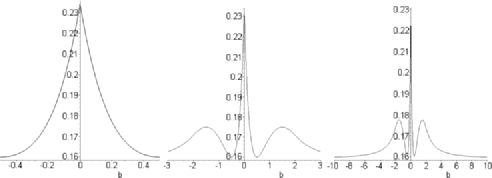
Figure 2: The behavior of the function $K(h^{*},b)$, for different values of $d$. Left panel $d=1/2$, middle panel $d=2$, right panel $d=10$.

A standardized maximin $T$-optimal discriminating design has masses $(1+d^{2})/4$, $(1-d^{2})/2$ and $(1+d^{2})/4$ at the points $-1$, $0$ and $1$, respectively.

In the case $1/2<d\leq 5\sqrt{10}/4$ the solution is given by $h^{*}=3/8$, $b^{*}=1/2$. Therefore the design with masses $5/16$, $3/8$ and $5/16$ at the points $-1$, $0$ and $1$ is a standardized maximin $T$-optimal discriminating design. The behavior of the function $K(h^{*},b)$ in this case is depicted in the middle panel of Figure 2.

In the case $d\in[\frac{5\sqrt{10}}{4},\infty]$ the structure of the solution changes again. For this interval the optimal pair $h^{*},b^{*}$ is obtained as a solution of the system

$$K(h,b)=K(h,d),\qquad\frac{\partial}{\partial b}K(h,b)=0,$$

and we find by a direct calculation that $b^{*}$ is the unique root of the equation

$$x^{4}+6x^{3}+\bigl{(}-2d^{2}+12\bigr{)}x^{2}+\bigl{(}-16d^{2}+8\bigr{)}x+8d^{2}=0$$

in the interval $[-4+2\sqrt{5},1/2]$. We have $h^{*}=b^{*}-\frac{(b^{*})^{2}}{2}$ and a standardized maximin $T$-optimal discriminating design has masses $1/2-b^{*}/2+(b^{*})^{2}/4$, $b^{*}-(b^{*})^{2}/2$, and $1/2-b^{*}/2+(b^{*})^{2}/4$ at the points $-1$, $0$ and $1$, respectively. In the limiting case $d=\infty$, that is, ${{\cal B}}=\mathbb{R}$, we have $b^{*}=-4+2\sqrt{5}$, $h^{*}=-22+10\sqrt{5}$ and a standardized maximin $T$-optimal discriminating design has masses $23/2-5\sqrt{5}$, $-22+10\sqrt{5}$, and $23/2-5\sqrt{5}$ at the points $-1$, $0$ and $1$, respectively. A typical case for the function $K(h^{*},b)$ in this case is depicted in the right panel of Figure 2 for $d=10$.

5.2 Bayesian $T$-optimal discriminating designs for quadratic regression

For the Bayesian $T$-optimality criterion a prior has to be chosen, and we propose to maximize an average of the efficiencies

$$\int_{-a}^{a}\operatorname{eff}_{T}(\xi,b)\,db$$

with respect to the uniform distribution on the interval $[-a,a]$. In criterion (6) this corresponds to an absolute continuous prior with density proportional to

$$f(b)=\cases{\displaystyle\frac{3(2+a)^{3}}{16a(12+6a+a^{2})}\frac{1}{\bar{R}(b)},&\quad$a\leq 2$,\cr\displaystyle\frac{3a}{17a-6}\frac{1}{\bar{R}(b)},&\quad$a\geq 2$,}$$

where $\bar{R}(b)$ is defined in (24) and the term depending on $a$ is the corresponding normalizing constant. By direct calculations we obtain

$$\int_{-a}^{a}b^{2}f(b)\,db=2\int_{0}^{a}b^{2}f(b)\,db=\cases{\displaystyle\frac{4a^{2}}{12+6a+a^{2}},&\quad$a\leq 2$,\vspace*{2pt}\cr\displaystyle\frac{6a^{2}-4a}{17a-6},&\quad$a\geq 2$.}$$

In order to apply Theorem 4.1 we consider $\beta_{B}=\min\{1,\int^{a}_{-a}b^{2}f(b)\,db\}$, and again three cases have to be considered: [(3)]

If $0<a\leq 2$ we have $\beta_{B}=\frac{4a^{2}}{12+6a+a^{2}}$ and a Bayesian $T$-optimal discriminating design has masses $\frac{5a^{2}+6a+12}{4(12+6a+a^{2})}$, $\frac{-3a^{2}+6a+12}{2(12+6a+a^{2})}$ and $\frac{5a^{2}+6a+12}{4(12+6a+a^{2})}$ at the points $-1$, $0$ and $1$.

If $2\leq a\leq\frac{7+\sqrt{33}}{4}$ we have $\beta_{B}=\frac{3a^{2}-4a}{17a-6}$, and a Bayesian $T$-optimal discriminating design has masses $\frac{6a^{2}+13a-6}{4(17a-6)}$, $\frac{-6a^{2}+21a-6}{2(17a-6)}$ and $\frac{6a^{2}+13a-6}{4(17a-6)}$ at the points $-1$, $0$ and $1$.

If $\frac{7+\sqrt{33}}{4}\leq a$ we have $\beta=1$ and a Bayesian $T$-optimal discriminating design has masses $1/2$ and $1/2$ at the points $-1$ and $1$.

5.3 Robust $T$-optimal discriminating designs for the Michaelis–Menten and EMAX model

In this section we briefly illustrate the application of the methodology in the situation described in Example 2.1, where the interest is in designs with good properties for discriminating between the Michaelis–Menten and EMAX model. We have calculated the standardized maximin $T$-optimal discriminating design for the Michaelis–Menten and EMAX model, where the region for the parameter $(\theta_{2,0},\theta_{2,1},\theta_{2,2})$ is given by $[-1.1,-0.2]\times\{1\}\times[2,6]$. The corresponding robust design is given by

$$\xi=\pmatrix{1&1.36&2\cr 0.410&0.205&0.385}.$$

As pointed out in Example 2.1, the efficiency of locally $T$-optimal discriminating designs can be low if some of the parameters of the regression models have been misspecified, and in Figure 3 we compare the performance of the locally and robust optimal discriminating designs if the true values are $\theta_{2,0}=-1$, $\theta_{2,1}=1$ and $\theta_{2,2}\in(2,6)$. We observe a substantial improvement by the standardized maximin $T$-optimal discriminating design. Other scenarios showed a similar picture and are not displayed for the sake of brevity.

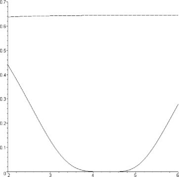
Figure 3: $T$-efficiency (4) of the standardized maximin optimal discriminating design (dotted line) and the locally $T$-optimal discriminating design for the Michaelis–Menten and EMAX model (calculated under the assumption $\theta_{2,0}=-1/4$, $\theta_{2,2}=1$, solid line). The “true” values are given by $\theta_{2,0}=-1$, $\theta_{2,1}=1$ and the efficiencies depend on the parameter $\theta_{2,2}\in(2,6)$.

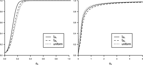
Figure 4: The power of the $F$-test for the hypothesis (26). Data are generated according to model (27). Left panel: normal distributed errors; right panel: normal distributed errors contaminated with $10\%$ Cauchy distributed errors.

5.4 Power and robustness

In order to demonstrate the effect of the optimal design on the power of the test for the corresponding hypothesis, we have conducted a small simulation study comparing Bayesian $T$-optimal discriminating designs and the commonly used uniform designs with respect to their discrimination properties for the models

$$\eta_{1}(x,\theta_{1})=\theta_{1,0};\qquad\eta_{2}(x,\theta_{2})=\theta_{2,0}+\theta_{2,1}x+\theta_{2,2}x^{2},$$ (25)

where the explanatory variable $x$ varies in the interval $[-1,1]$. For the construction of optimal discriminating designs we assume that the “true” ratio of the coefficients of $x$ and $x^{2}$ is an element of the interval $\mathcal{B}=[-1,1]$ or $\mathcal{B}=[-3,3]$. It follows from Section 5.2 that the Bayesian $T$-optimal discriminating designs with respect to the uniform distribution on the interval $[-1,1]$ and $[-3,3]$ are obtained as

$$\xi_{B_{1}}=\pmatrix{-1&0&1\vspace*{2pt}\cr\frac{23}{76}&\frac{15}{38}&\frac{23}{76}},\qquad\xi_{B_{2}}=\pmatrix{-1&0&1\vspace*{2pt}\cr\frac{29}{60}&\frac{1}{30}&\frac{29}{60}},$$

respectively. We assume that $60$ observations can be taken, which yield to the “realized” designs:

• $\xi_{B1}$: $18$, $24$, $18$ observations at the points $-1,0,1$ if $\mathcal{B}=[-1,1]$.

• $\xi_{B_{2}}$: $29$, $2$, $29$ observations at the points $-1,0,1$ if $\mathcal{B}=[-3,3]$.

For a comparison we use the uniform design:

• $6$ observations at the points $-1,-7/9,-5/9,\ldots,5/9,7/9,1$.

In the left part of Figure 4 we show the simulated rejection probabilities of the $F$-test for the hypothesis

$$H_{0}\dvtx\theta_{2,1}=\theta_{2,2}=0$$ (26)

(nominal level $5\%$) in the model

$$\eta_{2}(x,\theta_{2})=3+\tfrac{1}{2}\vartheta_{2}x+\vartheta_{2}x^{2},$$ (27)

where the errors are centered normal distributed with variance $\sigma^{2}=0.5$ (note that this means that the “true” ratio of the coefficients of $x$ and $x^{2}$ is given by $b=\frac{\theta_{2,1}}{\theta_{2,2}}=1/2$). All results are based on 250,000 simulation runs. We observe a notable improvement with respect to the power of the $F$-test if the experiments are conducted according to the $T$-optimal discriminating designs. The Bayesian $T$-optimal discriminating design with respect to the uniform distribution on $\mathcal{B}=[-1,1]$ yields a larger power than the Bayesian optimal design with respect to the uniform distribution on the interval $[-3,3]$. This corresponds to intuition because this design uses more precise and correct information regarding the unknown ratio $b=\theta_{2,1}/\theta_{2,2}$. In fact, using Bayesian $T$-optimal discriminating designs with respect to smaller intervals containing the “true” value $b=1/2$ yields even more powerful tests (these results are not depicted for the sake of brevity).

It was pointed out by a referee that it might be of interest to investigate the sensitivity of the $F$-test for the different designs with respect to influential observations. For this purpose we have performed the same simulation where $10\%$ of the normal distributed errors are replaced by Cauchy distributed random variables. The corresponding results are shown in the right part of Figure 4, and the results change substantially. We observe a loss in power for all three designs. Under the null hypothesis the Bayesian $T$-optimal discriminating designs yield a slightly conservative test while the $F$-test based on the uniform design rejects the null hypothesis too often. Because of continuity of the power function this phenomenon is also observed for other values of $\vartheta_{2}$. On the other hand, for large values of $\vartheta_{2}$ the Bayesian $T$-optimal discriminating design $\xi_{B_{1}}$ with respect to the uniform distribution on the interval $[-1,1]$ and the uniform design yield a similar power of the $F$-test, while a slightly lower power is observed for the $F$-test based on the Bayesian $T$-optimal discriminating design $\xi_{B_{2}}$ with respect to the uniform distribution on the interval $[-3,3]$.

Model (27) keeps the ratio of the coefficients of $x$ and $x^{2}$ constant and in the second example of this section we consider an alternative data generating model, that is,

$$\eta_{2}(x,\theta_{2})=3+\tfrac{1}{8}x+\vartheta_{2}x^{2},$$ (28)

where $\vartheta_{2}$ varies in the interval $[-0.5,0.5]$, which means that the “true” ratio $b$ of the coefficients of $x$ and $x^{2}$ varies in $\mathbb{R}\setminus[-0.25,0.25]$. In particular the ratio of the coefficients of $x$ and $x^{2}$ in model (28) can attain values which are not contained in the set $\mathcal{B}$ used for the construction of the Bayesian $T$-optimal discriminating designs. Again $60$ observations are generated according to the designs specified in the previous paragraph and the corresponding results are depicted in Figure 5. Note that none of the values $\vartheta_{2}\in[-0.5,0.5]$ corresponds to the null hypothesis and consequently the curves show only the power under certain alternatives. We observe from the left panel in Figure 5 that for normally distributed

Figure 5: The power of the $F$-test for the hypothesis (26). Data are generated according to model (28). Left panel: normal distributed errors; right panel: normal distributed errors contaminated with $10\%$ Cauchy distributed errors.

errors the Bayesian $T$-optimal discriminating design $\xi_{B_{1}}$ with respect to the uniform distribution on the interval $[-1,1]$ yields uniformly more power than the uniform design. On the other hand the Bayesian $T$-optimal discriminating design $\xi_{B_{2}}$ with respect to the uniform distribution on the interval $[-3,3]$ is preferable to the uniform design if $\vartheta_{2}\leq 0.3$, while for larger values of $\vartheta_{2}$ the $F$-test based on the uniform design is more powerful. Moreover, if $\vartheta_{2}\leq 0.1$ the design $\xi_{B_{2}}$ is even better than the design $\xi_{B_{1}}$. This corresponds to intuition, because the design $\xi_{B_{2}}$ is very close to the optimal design for discriminating between a constant and a linear regression model, which puts equal masses at the points $-1$ and $1$. For Cauchy distributed errors we observe a very similar behavior, where the power is smaller due to the contamination of the normal distribution.

References

- Asprey and Macchietto (2000) {barticle}[auto:STB—2013/06/05—13:45:01] \bauthor\bsnmAsprey, \bfnmS. P.\binitsS. P. and \bauthor\bsnmMacchietto, \bfnmS.\binitsS. (\byear2000). \btitleStatistical tools for optimal dynamic model building. \bjournalComputers and Chemical Engineering \bvolume24 \bpages1261–1267. \bptokimsref \endbibitem
- Atkinson (2010) {bincollection}[auto:STB—2013/06/05—13:45:01] \bauthor\bsnmAtkinson, \bfnmA. C.\binitsA. C. (\byear2010). \btitleThe non-uniqueness of some designs for discriminating between two polynomial models in one variable. In \bbooktitleMODA 9, Advances in Model-Oriented Design and Analysis \bpages9–16. \bpublisherSpringer, \blocationHeidelberg. \bptokimsref \endbibitem
- Atkinson, Bogacka and Bogacki (1998) {barticle}[auto:STB—2013/06/05—13:45:01] \bauthor\bsnmAtkinson, \bfnmA. C.\binitsA. C., \bauthor\bsnmBogacka, \bfnmB.\binitsB. and \bauthor\bsnmBogacki, \bfnmM. B.\binitsM. B. (\byear1998). \btitle- and -optimum designs for the kinetics of a reversible chemical reaction. \bjournalChemometrics and Intelligent Laboratory Systems \bvolume43 \bpages185–198. \bptokimsref \endbibitem
- Atkinson and Fedorov (1975a) {barticle}[mr] \bauthor\bsnmAtkinson, \bfnmA. C.\binitsA. C. and \bauthor\bsnmFedorov, \bfnmV. V.\binitsV. V. (\byear1975a). \btitleThe design of experiments for discriminating between two rival models. \bjournalBiometrika \bvolume62 \bpages57–70. \bidissn=0006-3444, mr=0370955 \bptokimsref \endbibitem
- Atkinson and Fedorov (1975b) {barticle}[mr] \bauthor\bsnmAtkinson, \bfnmA. C.\binitsA. C. and \bauthor\bsnmFedorov, \bfnmV. V.\binitsV. V. (\byear1975b). \btitleOptimal design: Experiments for discriminating between several models. \bjournalBiometrika \bvolume62 \bpages289–303. \bidissn=0006-3444, mr=0381163 \bptokimsref \endbibitem
- Bretz, Pinheiro and Branson (2005) {barticle}[mr] \bauthor\bsnmBretz, \bfnmF.\binitsF., \bauthor\bsnmPinheiro, \bfnmJ. C.\binitsJ. C. and \bauthor\bsnmBranson, \bfnmM.\binitsM. (\byear2005). \btitleCombining multiple comparisons and modeling techniques in dose-response studies. \bjournalBiometrics \bvolume61 \bpages738–748. \biddoi=10.1111/j.1541-0420.2005.00344.x, issn=0006-341X, mr=2196162 \bptokimsref \endbibitem
- Chaloner and Verdinelli (1995) {barticle}[mr] \bauthor\bsnmChaloner, \bfnmKathryn\binitsK. and \bauthor\bsnmVerdinelli, \bfnmIsabella\binitsI. (\byear1995). \btitleBayesian experimental design: A review. \bjournalStatist. Sci. \bvolume10 \bpages273–304. \bidissn=0883-4237, mr=1390519 \bptokimsref \endbibitem
- Chernoff (1953) {barticle}[mr] \bauthor\bsnmChernoff, \bfnmHerman\binitsH. (\byear1953). \btitleLocally optimal designs for estimating parameters. \bjournalAnn. Math. Statist. \bvolume24 \bpages586–602. \bidissn=0003-4851, mr=0058932 \bptokimsref \endbibitem
- Cornish-Bowden (1965) {bbook}[auto:STB—2013/06/05—13:45:01] \bauthor\bsnmCornish-Bowden, \bfnmA.\binitsA. (\byear1965). \btitleFundamentals of Enzyme Kinetics, \beditionrev. ed. \bpublisherPortland Press, \blocationLondon. \bptokimsref \endbibitem
- Danesi et al. (2002) {barticle}[auto:STB—2013/06/05—13:45:01] \bauthor\bsnmDanesi, \bfnmR.\binitsR., \bauthor\bsnmInnocenti, \bfnmF.\binitsF., \bauthor\bsnmFogli, \bfnmS.\binitsS., \bauthor\bsnmGennari, \bfnmA.\binitsA., \bauthor\bsnmBaldini, \bfnmE.\binitsE., \bauthor\bsnmDi Paolo, \bfnmA.\binitsA., \bauthor\bsnmSalvadori, \bfnmB.\binitsB., \bauthor\bsnmBocci, \bfnmG.\binitsG., \bauthor\bsnmConte, \bfnmP. F.\binitsP. F. and \bauthor\bsnmDel Tacca, \bfnmM.\binitsM. (\byear2002). \btitlePharmacokinetics and pharmacodynamics of combination chemotherapy with paclitaxel and epirubicin in breast cancer patients. \bjournalBr. J. Clin. Pharmacol. \bvolume53 \bpages508–518. \bptokimsref \endbibitem
- Dette (1994) {barticle}[mr] \bauthor\bsnmDette, \bfnmHolger\binitsH. (\byear1994). \btitleDiscrimination designs for polynomial regression on compact intervals. \bjournalAnn. Statist. \bvolume22 \bpages890–903. \biddoi=10.1214/aos/1176325501, issn=0090-5364, mr=1292546 \bptokimsref \endbibitem
- Dette (1995) {barticle}[mr] \bauthor\bsnmDette, \bfnmHolger\binitsH. (\byear1995). \btitleOptimal designs for identifying the degree of a polynomial regression. \bjournalAnn. Statist. \bvolume23 \bpages1248–1266. \biddoi=10.1214/aos/1176324708, issn=0090-5364, mr=1353505 \bptokimsref \endbibitem
- Dette (1997) {barticle}[mr] \bauthor\bsnmDette, \bfnmHolger\binitsH. (\byear1997). \btitleDesigning experiments with respect to “standardized” optimality criteria. \bjournalJ. R. Stat. Soc. Ser. B Stat. Methodol. \bvolume59 \bpages97–110. \biddoi=10.1111/1467-9868.00056, issn=0035-9246, mr=1436556 \bptokimsref \endbibitem
- Dette, Haines and Imhof (2007) {barticle}[mr] \bauthor\bsnmDette, \bfnmHolger\binitsH., \bauthor\bsnmHaines, \bfnmLinda M.\binitsL. M. and \bauthor\bsnmImhof, \bfnmLorens A.\binitsL. A. (\byear2007). \btitleMaximin and Bayesian optimal designs for regression models. \bjournalStatist. Sinica \bvolume17 \bpages463–480. \bidissn=1017-0405, mr=2408676 \bptokimsref \endbibitem
- Dette and Haller (1998) {barticle}[mr] \bauthor\bsnmDette, \bfnmHolger\binitsH. and \bauthor\bsnmHaller, \bfnmGerd\binitsG. (\byear1998). \btitleOptimal designs for the identification of the order of a Fourier regression. \bjournalAnn. Statist. \bvolume26 \bpages1496–1521. \biddoi=10.1214/aos/1024691251, issn=0090-5364, mr=1647689 \bptokimsref \endbibitem
- Dette, Melas and Wong (2005) {barticle}[mr] \bauthor\bsnmDette, \bfnmHolger\binitsH., \bauthor\bsnmMelas, \bfnmViatcheslav B.\binitsV. B. and \bauthor\bsnmWong, \bfnmWeng Kee\binitsW. K. (\byear2005). \btitleOptimal design for goodness-of-fit of the Michaelis–Menten enzyme kinetic function. \bjournalJ. Amer. Statist. Assoc. \bvolume100 \bpages1370–1381. \biddoi=10.1198/016214505000000600, issn=0162-1459, mr=2236448 \bptokimsref \endbibitem
- Dette, Melas and Shpilev (2012) {barticle}[mr] \bauthor\bsnmDette, \bfnmHolger\binitsH., \bauthor\bsnmMelas, \bfnmViatcheslav B.\binitsV. B. and \bauthor\bsnmShpilev, \bfnmPetr\binitsP. (\byear2012). \btitle-optimal designs for discrimination between two polynomial models. \bjournalAnn. Statist. \bvolume40 \bpages188–205. \biddoi=10.1214/11-AOS956, issn=0090-5364, mr=3013184 \bptokimsref \endbibitem
- Dette and Studden (1997) {bbook}[mr] \bauthor\bsnmDette, \bfnmHolger\binitsH. and \bauthor\bsnmStudden, \bfnmWilliam J.\binitsW. J. (\byear1997). \btitleThe Theory of Canonical Moments with Applications in Statistics, Probability, and Analysis. \bpublisherWiley, \blocationNew York. \bidmr=1468473 \bptokimsref \endbibitem
- Dette and Titoff (2009) {barticle}[mr] \bauthor\bsnmDette, \bfnmHolger\binitsH. and \bauthor\bsnmTitoff, \bfnmStefanie\binitsS. (\byear2009). \btitleOptimal discrimination designs. \bjournalAnn. Statist. \bvolume37 \bpages2056–2082. \biddoi=10.1214/08-AOS635, issn=0090-5364, mr=2533479 \bptokimsref \endbibitem
- Foo and Duffull (2011) {bincollection}[auto:STB—2013/06/05—13:45:01] \bauthor\bsnmFoo, \bfnmL. K.\binitsL. K. and \bauthor\bsnmDuffull, \bfnmS.\binitsS. (\byear2011). \btitleOptimal design of pharmacokinetic-pharmacodynamic studies. In \bbooktitlePharmacokinetics in Drug Development, Advances and Applications. \bpublisherSpringer, \blocationNew York. \bptokimsref \endbibitem
- Gaffke (1987) {barticle}[mr] \bauthor\bsnmGaffke, \bfnmNorbert\binitsN. (\byear1987). \btitleFurther characterizations of design optimality and admissibility for partial parameter estimation in linear regression. \bjournalAnn. Statist. \bvolume15 \bpages942–957. \biddoi=10.1214/aos/1176350485, issn=0090-5364, mr=0902238 \bptokimsref \endbibitem
- Hill (1978) {barticle}[auto:STB—2013/06/05—13:45:01] \bauthor\bsnmHill, \bfnmP. D.\binitsP. D. (\byear1978). \btitleA review of experimental design procedures for regression model discrimination. \bjournalTechnometrics \bvolume20 \bpages15–21. \bptokimsref \endbibitem
- Hunter and Reiner (1965) {barticle}[mr] \bauthor\bsnmHunter, \bfnmWilliam G.\binitsW. G. and \bauthor\bsnmReiner, \bfnmAlbey M.\binitsA. M. (\byear1965). \btitleDesigns for discriminating between two rival models. \bjournalTechnometrics \bvolume7 \bpages307–323. \bidissn=0040-1706, mr=0192615 \bptokimsref \endbibitem
- Karlin and Studden (1966) {bbook}[mr] \bauthor\bsnmKarlin, \bfnmSamuel\binitsS. and \bauthor\bsnmStudden, \bfnmWilliam J.\binitsW. J. (\byear1966). \btitleTchebycheff Systems: With Applications in Analysis and Statistics. \bseriesPure and Applied Mathematics \bvolumeXV. \bpublisherWiley, \blocationNew York. \bidmr=0204922 \bptokimsref \endbibitem
- Kiefer (1974) {barticle}[mr] \bauthor\bsnmKiefer, \bfnmJ.\binitsJ. (\byear1974). \btitleGeneral equivalence theory for optimum designs (approximate theory). \bjournalAnn. Statist. \bvolume2 \bpages849–879. \bidissn=0090-5364, mr=0356386 \bptokimsref \endbibitem
- Müller and Pázman (1998) {barticle}[mr] \bauthor\bsnmMüller, \bfnmChristine H.\binitsC. H. and \bauthor\bsnmPázman, \bfnmAndrej\binitsA. (\byear1998). \btitleApplications of necessary and sufficient conditions for maximin efficient designs. \bjournalMetrika \bvolume48 \bpages1–19. \bidissn=0026-1335, mr=1647889 \bptokimsref \endbibitem
- Osborne and Rubinstein (1994) {bbook}[mr] \bauthor\bsnmOsborne, \bfnmMartin J.\binitsM. J. and \bauthor\bsnmRubinstein, \bfnmAriel\binitsA. (\byear1994). \btitleA Course in Game Theory. \bpublisherMIT Press, \blocationCambridge, MA. \bidmr=1301776 \bptokimsref \endbibitem
- Ponce de Leon and Atkinson (1991) {barticle}[mr] \bauthor\bparticlePonce de \bsnmLeon, \bfnmA. C.\binitsA. C. and \bauthor\bsnmAtkinson, \bfnmA. C.\binitsA. C. (\byear1991). \btitleOptimum experimental design for discriminating between two rival models in the presence of prior information. \bjournalBiometrika \bvolume78 \bpages601–608. \biddoi=10.1093/biomet/78.3.601, issn=0006-3444, mr=1130928 \bptokimsref \endbibitem
- Pukelsheim and Rieder (1992) {barticle}[mr] \bauthor\bsnmPukelsheim, \bfnmFriedrich\binitsF. and \bauthor\bsnmRieder, \bfnmSabine\binitsS. (\byear1992). \btitleEfficient rounding of approximate designs. \bjournalBiometrika \bvolume79 \bpages763–770. \biddoi=10.1093/biomet/79.4.763, issn=0006-3444, mr=1209476 \bptokimsref \endbibitem
- Song and Wong (1999) {barticle}[mr] \bauthor\bsnmSong, \bfnmDale\binitsD. and \bauthor\bsnmWong, \bfnmWeng Kee\binitsW. K. (\byear1999). \btitleOn the construction of -optimal designs. \bjournalStatist. Sinica \bvolume9 \bpages263–272. \bidissn=1017-0405, mr=1678893 \bptokimsref \endbibitem
- Spruill (1990) {barticle}[mr] \bauthor\bsnmSpruill, \bfnmM. C.\binitsM. C. (\byear1990). \btitleGood designs for testing the degree of a polynomial mean. \bjournalSankhyā Ser. B \bvolume52 \bpages67–74. \bidissn=0581-5738, mr=1178893 \bptokimsref \endbibitem
- Stigler (1971) {barticle}[auto:STB—2013/06/05—13:45:01] \bauthor\bsnmStigler, \bfnmS.\binitsS. (\byear1971). \btitleOptimal experimental design for polynomial regression. \bjournalJ. Amer. Statist. Assoc. \bvolume66 \bpages311–318. \bptokimsref \endbibitem
- Studden (1982) {barticle}[mr] \bauthor\bsnmStudden, \bfnmW. J.\binitsW. J. (\byear1982). \btitleSome robust-type -optimal designs in polynomial regression. \bjournalJ. Amer. Statist. Assoc. \bvolume77 \bpages916–921. \bidissn=0162-1459, mr=0686418 \bptokimsref \endbibitem
- Studden (1989) {barticle}[mr] \bauthor\bsnmStudden, \bfnmW. J.\binitsW. J. (\byear1989). \btitleNote on some -optimal designs for polynomial regression. \bjournalAnn. Statist. \bvolume17 \bpages618–623. \biddoi=10.1214/aos/1176347129, issn=0090-5364, mr=0994254 \bptokimsref \endbibitem
- Szegö (1959) {bbook}[mr] \bauthor\bsnmSzegö, \bfnmGabor\binitsG. (\byear1959). \btitleOrthogonal Polynomials, \beditionrev. ed. \bseriesAmerican Mathematical Society Colloquium Publications \bvolume23. \bpublisherAmer. Math. Soc., \blocationProvidence, RI. \bidmr=0106295 \bptokimsref \endbibitem
- Tommasi and López-Fidalgo (2010) {barticle}[mr] \bauthor\bsnmTommasi, \bfnmC.\binitsC. and \bauthor\bsnmLópez-Fidalgo, \bfnmJ.\binitsJ. (\byear2010). \btitleBayesian optimum designs for discriminating between models with any distribution. \bjournalComput. Statist. Data Anal. \bvolume54 \bpages143–150. \biddoi=10.1016/j.csda.2009.07.022, issn=0167-9473, mr=2558465 \bptokimsref \endbibitem
- Uciński and Bogacka (2005) {barticle}[mr] \bauthor\bsnmUciński, \bfnmDariusz\binitsD. and \bauthor\bsnmBogacka, \bfnmBarbara\binitsB. (\byear2005). \btitle-optimum designs for discrimination between two multiresponse dynamic models. \bjournalJ. R. Stat. Soc. Ser. B Stat. Methodol. \bvolume67 \bpages3–18. \biddoi=10.1111/j.1467-9868.2005.00485.x, issn=1369-7412, mr=2136636 \bptokimsref \endbibitem
- Waterhouse et al. (2008) {barticle}[mr] \bauthor\bsnmWaterhouse, \bfnmT. H.\binitsT. H., \bauthor\bsnmWoods, \bfnmD. C.\binitsD. C., \bauthor\bsnmEccleston, \bfnmJ. A.\binitsJ. A. and \bauthor\bsnmLewis, \bfnmS. M.\binitsS. M. (\byear2008). \btitleDesign selection criteria for discrimination/estimation for nested models and a binomial response. \bjournalJ. Statist. Plann. Inference \bvolume138 \bpages132–144. \biddoi=10.1016/j.jspi.2007.05.017, issn=0378-3758, mr=2369620 \bptokimsref \endbibitem
- Wiens (2009) {barticle}[mr] \bauthor\bsnmWiens, \bfnmDouglas P.\binitsD. P. (\byear2009). \btitleRobust discrimination designs. \bjournalJ. R. Stat. Soc. Ser. B Stat. Methodol. \bvolume71 \bpages805–829. \biddoi=10.1111/j.1467-9868.2009.00711.x, issn=1369-7412, mr=2750096 \bptokimsref \endbibitem
- Wiens (2010) {barticle}[mr] \bauthor\bsnmWiens, \bfnmDouglas P.\binitsD. P. (\byear2010). \btitleRobustness of design for the testing of lack of fit and for estimation in binary response models. \bjournalComput. Statist. Data Anal. \bvolume54 \bpages3371–3378. \biddoi=10.1016/j.csda.2009.03.001, issn=0167-9473, mr=2727759 \bptokimsref \endbibitem