Control of transport in higher dimensional systems via dynamical decoupling of degrees of freedom with quasiperiodic driving fields

Abstract

We consider the problem of the control of transport in higher dimensional periodic structures by applied ac fields. In a generic crystal, transverse degrees of freedom are coupled, and this makes the control of motion difficult to implement. We show, both with simulations and with an analytical functional expansion on the driving amplitudes, that the use of quasiperiodic driving significantly suppresses the coupling between transverse degrees of freedom. This allows a precise control of the transport, and does not require a detailed knowledge of the crystal geometry.

I Introduction

Periodic and quasiperiodic structures, both in time and in space, exhibit completely different properties. For the case of spatial quasiperiodicity, it is well established that quasiperiodic crystals exhibit properties which are very different from their periodic counterpart. In particular, transport properties, which are the main focus of this work, are significantly modified in the transition from a periodic structure to a quasi-periodic one. The transition from a ballistic regime in a periodic crystal to a regime of anomalous diffusion in a perfect quasicrystal well highlights the profound difference between the two structures. Mathematically, a quasicrystal can be treated as a periodic structure embedded in an hyperspace of higher dimension. That is, the effective dimensionality of the system is changed in the transition from periodicity to quasiperiodicity. This is the feature that, in the time-domain, will be central to our analysis.

In this work we consider the problem of the control of transport in higher-dimensional crystals via ac driving fields reimann02 ; hanmar09 . In a generic crystal transverse degrees of freedom are coupled, and this makes the control of motion difficult to implement. Inspired by the above unique feature of quasiperiodic structures, we examine the case of a periodic spatial lattice and a quasiperiodic driving. We demonstrate, both with simulations and with a quite general functional expansion on the driving amplitudes, that the use of quasiperiodic driving leads to a dynamical decoupling of degrees of freedom, whereby the coupling between transverse degrees of freedom is significantly suppressed. This allows a precise control of the transport, independently of the lattice structure.

II Model and definitions

In the simulations, we choose as an example the dynamics of a classical particle described by the Langevin equation

$$m\ddot{{\bf r}}=-\alpha\dot{{\bf r}}-\nabla U({\bf r})+{\bf F}(t)+{\bf\xi}(t),$$ (1)

where ${\bf r}=(x,y)$ is the coordinate vector of the particle, $m$ is its mass, $\alpha$ the friction coefficient, ${\bf\xi}=(\xi_{x},\xi_{y})$ a fluctuating force modeled by two independent Gaussian white noises, $\langle\xi_{i}(t)\xi_{j}(t^{\prime})\rangle=2D\delta(t-t^{\prime})\delta_{ij}$ ($i,j=x,y$), ${\bf F}(t)$ an applied time-dependent driving to be specified later on, and $U({\bf r})$ a two-dimensional space-periodic potential that is also spatially symmetric in both directions $x$ and $y$. We have considered first the potential

$$U({\bf r})=U_{0}\cos(kx)[1+\cos(2ky)],$$ (2)

which defines a rectangular lattice. Throughout the paper, reduced units are assumed so that $m=k=U_{0}=1$. In these units, the friction coefficient and the noise strength were fixed to $\alpha=0.1$ and $D=0.5$.

This system model contains noise, dissipation, and finite inertia, which are important ingredients in the modelling of the experiments using 2D optical lattices presented in Ref. lebren09 . Note however that the main conclusions reported in this paper are supported by a general analytical calculation based only on symmetry considerations, and, thus, do not depend on the specific details of the dynamics (1), or if the particle is classical or quantum.

The quantity of interest is the directed current, formally defined as

$$\langle{\bf v}\rangle=\lim_{t\rightarrow\infty}\frac{\langle{\bf r}(t)-{\bf r}(0)\rangle}{t}.$$ (3)

Such a current is generated by the application of an appropriate ac force. We consider here a driving consisting of two orthogonal bi-harmonic drives along the $x$ and $y$ directions:

$$F_{x}(t) = A_{x}[\cos(\omega_{1}t)+\cos(2\omega_{1}t+\phi_{1})],$$ (4a)

$$F_{y}(t) = A_{y}[\cos(\omega_{2}t)+\cos(2\omega_{2}t+\phi_{2})],$$ (4b)

with $\phi_{1}=\phi_{2}=\pi/2$. Previous work for one-dimensional systems has shown that the biharmonic driving, breaking all the system symmetries, is able to produce a current, whose amplitude and direction can be controlled via the amplitude and the frequency of the strength of the driving fabio ; chialvo ; dykman ; flayev00 ; machura ; cubleb10 ; wiccub11 . In the absence of coupling between transverse degrees of freedom, ac driving of the form of Eq. (4) allows a precise control of transport through the 2D lattice.

It is important to note that, numerically or in an experiment, the limit (3) cannot be carried out to infinity, but to a sufficiently large observation time $T_{s}$. This has important implications on whether two driving frequencies $\omega_{1}$ and $\omega_{2}$ can be regarded as commensurate (i.e. $\omega_{2}/\omega_{1}$ is a rational number) or effectively incommensurate (quasiperiodic driving) on the time scale of the simulation. Obviously, a periodic driving with a rational ratio $\omega_{2}/\omega_{1}$, specifically chosen with a period much larger than $T_{s}$, cannot be distinguished from one with an irrational ratio. The periodic and quasiperiodic regimes are then determined by the observation time $T_{s}$, as we illustrate in the next section.

III Control of transverse coupling

In the absence of a coupling between the $x$ and $y$ direction, a driving of the form of Eq. (4) allows a precise control of transport through the 2D lattice. However, for a generic lattice the transverse degrees of freedom are effectively coupled. This can be shown by considering the minimal case of a split biharmonic driving denzol08 ; lebren09 : $F_{x}(t)=A\cos(\omega_{1}t)$, $F_{y}(t)=A\cos(\omega_{2}t+\pi/2)$ with $\omega_{2}=2\omega_{1}$. For sufficiently large times, the system approaches an attractor solution which is time periodic, with period $T=2\pi/\omega_{1}$. Invariance under the symmetry transformation $(x,y,t)\rightarrow(-x,y,t+T/2)$ forbids transport along the $x$ direction. On the other hand, the $y$ component of the driving force breaks all symmetries of the system reimann02 ; denzol08 , and thus directed transport is expected along the $y$ direction. In our simulations, with the driving parameters $A=5$, $\omega_{1}=\omega_{2}/2=\sqrt{2}$, we obtained $\langle v_{x}\rangle=-0.0001\pm 0.0004$ and $\langle v_{y}\rangle=-0.0281\pm 0.0003$, confirming the symmetry analysis. The uncertainties were estimated from the statistics of 39000 independent trajectories. Note that if the system were one-dimensional, e.g along the $y$ direction, the single harmonic driving $F_{y}(t)$ would not induce a current, because the system would be symmetric under the transformation $(y,t)\rightarrow(-y,t+\pi/\omega_{2})$. This analysis shows that there is a strong coupling between the $x$ and $y$ directions. The particle needs to explore orbits the $x$ direction in order to produce an average drift in the $y$ direction denzol08 .

As a central result of our analysis, we now show that the transverse coupling can be effectively suppressed by replacing the periodic driving considered so far by a quasiperiodic one with the same functional form, as obtained by choosing a driving frequency $\omega_{2}$ that is incommensurate with respect to $\omega_{1}$. While the variation in frequency required to obtain the transition from a periodic to a quasiperiodic driving may be tiny (few parts per thousand in the case studies presented in the following), the change in the type of driving has profound effects on the dynamics. In fact, the transition to quasiperiodicity determines an effective change in the dimensionality of the system. Formally, the compact phase space is extended neupik02 to include the variables $\psi_{1}=\omega_{1}t$ and $\psi_{2}=\omega_{2}t$. This extension removes the explicit time-dependence of the problem, turning the focus from time-dependent to stationary solutions (and thus time-periodic with period zero). Since the irrationality of the frequency ratio provides ergodic motion in the compact subspace $(\psi_{1},\psi_{2})$ arnold74 , it is natural to assume neupik02 that the dynamics in the extended phase space is ergodic. As a consequence, the variables $\psi_{1}$ and $\psi_{2}$ can be treated as effectively independent variables in the symmetry analysis. The system, driven by the split biharmonic force with $\omega_{2}/\omega_{2}$ irrational, is symmetric under the transformation $(x,y,\psi_{1},\psi_{2})\rightarrow(-x,-y,\psi_{1}+\pi,\psi_{2}+\pi)$, and no directed current should appear in any direction. The simulations confirm this prediction for the driving frequencies $\omega_{1}=\sqrt{2}$ and $\omega_{2}=2.82$, with an observation time of $T_{s}=10^{5}$, resulting in a zero (within the error) current with $\langle v_{x}\rangle=-0.0001\pm 0.0002$ and $\langle v_{y}\rangle=-0.0002\pm 0.0003$. This shows that the coupling between transverse degrees of freedom can be controlled and suppressed by using quasiperiodic ac drivings. Remarkably, a small variation in frequency ($\omega_{1}$ and $\omega_{2}/2$ differ in less than 0.3%) is sufficient for the system to react as if $\omega_{2}/\omega_{1}$ were irrational, displaying a very different physical behavior when compared to the rational case $\omega_{1}=\omega_{2}/2$. The present result also represents the generalization to 2D of the symmetry analysis for 1D quasiperiodically driven systems introduced in Refs. fladen04 ; gomden06 ; gombro07 .

So far we only discussed the current at the exact value of the frequency corresponding to quasiperiodicity. For finite-time real (numerical) experiments, as the case considered here, it is interesting to examine the dependence on the current generated along the $y$ direction on the frequency of the control fields. Such a dependence is shown in Figure 1, and it can be precisely explained by the finite observation time $T_{s}$. The symmetry analysis discussed earlier, which assumes an infinite $T_{s}$, predicts that only the value $\omega_{2}=2\sqrt{2}$ of those shown in Fig. 1 produces a current different from zero. Correspondingly, the Fourier cosine transform of the single harmonic $F(t)=\cos(\omega_{0}t)$ is proportional to a Dirac delta centered at $\omega_{0}$,

$$\int_{0}^{\infty}dt\,\cos(\omega_{0}t)\cos(\omega t)=\pi\delta(\omega-\omega_{0}).$$ (5)

However, when the finite observation time $T_{s}$ is taken into account, the Fourier transform has to be replaced by

$$\int_{0}^{T_{s}}dt\,\cos(\omega_{0}t)\cos(\omega t)=\pi\delta_{1/T_{s}}(\omega+\omega_{0})+\pi\delta_{1/T_{s}}(\omega-\omega_{0}),$$ (6)

where $\delta_{\epsilon}(x)=\mathrm{sinc}(x/\epsilon)/(\pi\epsilon)$ is a well known representation of the delta function with the sinc function $\mathrm{sinc}(x)=\sin(x)/x$. The first delta function of the right-hand side of (6) is irrelevant because the frequency $\omega$ in the Fourier cosine transform is only defined for $\omega\geq 0$. Therefore, we would expect that the system response also shows a similar frequency broadening in the neighborhood of $\omega_{2}=2\omega_{1}$ due to the finite duration $T_{s}$,

$$\langle v_{y}\rangle\approx v_{0}\cdot\mathrm{sinc}[(\omega_{2}-2\omega_{1})T_{s}],$$ (7)

where $v_{0}$ is the value of $\langle v_{y}\rangle$ when $\omega_{2}=2\omega_{1}$ (note that $\mathrm{sinc}(0)=1$). The lines in Fig. 1 show that the shape is well described by this approximation. The width $\Delta\omega$ of the resonance around the value which defines quasiperiodicity is simply the frequency resolution introduced by the finite duration $T_{s}$ of the measurement: $\Delta\omega=2\pi/T_{s}$. For a real experiment, such a width controls the frequency window within which the driving could be regarded approximately as periodic, i.e. it defines the frequency jump required to move from the periodic driving regime to the quasiperiodic one.

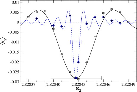
Figure 1: (Color online) Simulation results for the $y$ component of the current as a function of the frequency $\omega_{2}$ for a system driven by a split bi-harmonic driving with $\omega_{1}=\sqrt{2}$. The empty diamonds correspond to an observation time of $T_{s}=10^{5}$, while the filled diamonds to $T_{s}=5\cdot 10^{5}$. The horizontal error bars centered at $\omega_{2}=2\sqrt{2}$ indicate $\Delta\omega=2\pi/T_{s}$ with $T_{s}=10^{5}$ (solid line) and $T_{s}=5\cdot 10^{5}$ (dashed line). The lines are the prediction given by (7) with $T_{s}=10^{5}$ (solid line) and $T_{s}=5\cdot 10^{5}$ (dashed line).

IV Control of transport in 2D with quasiperiodic driving

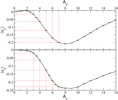
Figure 2: (Color online) Simulation results for the 1D current, as obtained by applying a biharmonic driving along one direction only, as a function of the amplitude of the driving for the relevant direction. Using the notations as from Eq. (4), the parameters of the calculations are as follows. Top panel: $\langle v_{y}\rangle$ vs. $A_{y}$ for $A_{x}=0$; bottom panel: $\langle v_{x}\rangle$ vs. $A_{x}$ for $A_{y}=0$. In all cases $\omega_{1}=\omega_{2}=\sqrt{2}$. The solid lines are a guide to the eye. The dotted lines (red) mark a set of reference values of $A_{x}$ and $A_{y}$.

We now consider the problem of the control of transport in 2D with ac drivings. We analyze the simplest case of drivings breaking all the relevant symmetries, the double biharmonic driving, Eq. (4).

Previous work lebren09 demonstrated that it is possible to produce directed motion along an arbitrary direction of the 2D substrate by using ac driving forces. However, the mechanism shown in that work lacks the essential feature of a control protocol: predictability. Indeed, because of the coupling between transverse degrees of freedom, and the nonlinearity of the mechanism of rectification along each direction, it is impossible, given the parameters of the driving, to predict in a straightforward way the direction along which directed motions will be produced. Only a complete calculation, which also requires the exact knowledge of the geometry of the 2D structure, can reveal the direction of the current which is in general different from the direction corresponding to the vector sum of the forces oscillating in the two directions.

As it will be shown here, the use of quasiperiodic ac fields leads instead to a simple control protocol, which produces a current closer to a direction corresponding to the vector sum of the forces oscillating in the two directions, independently of the lattice geometry.

As a starting point, we consider the 1D current, as obtained by applying a biharmonic driving along one direction only. Numerical results for this case are reported in Fig. 2. The observation time was fixed to $T_{s}=10^{5}$. Two general remarks are in order. First, the sign of the current (negative for the considered parameters) is not important as it can be controlled by inverting the values of $A_{x}$ and/or $A_{y}$ or changing the values of $\phi_{1}$ and/or $\phi_{2}$ to $\phi_{1}\rightarrow\phi_{1}+\pi$ and $\phi_{2}\rightarrow\phi_{2}+\pi$. In either case, the sign of the current component $\langle v_{x}\rangle$ and/or $\langle v_{y}\rangle$ would be reversed. Second, it can be seen that for the relatively small values of the driving amplitudes (about $A_{x},A_{y}\leq 2$ in Fig. 2), the current remains very small. A functional expansion on the driving amplitude confirms that no current is generated at the first reimann02 (linear response theory) and second order on the driving amplitude quicue10 . Furthermore, Fig. 2 shows that the current in each direction presents a non-monotonous behavior with the driving amplitudes (showing two minima at about $A_{x},A_{y}\sim 8$). This is also expected, because for very large driving amplitudes the potential can be neglected and thus, the potential’s nonlinearity, which determines the current generation, diminishes, eventually leading to the disappearance of the current for large enough driving. Since we are interested in controlling the directed current through the driving amplitudes, it will suffice to restrict ourselves to the range of parameter values defined by $3\leq A_{x},A_{y}\leq 7$.

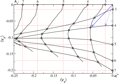
Figure 3: (Color online) Simulation results for the rectangular potential of Eq. (2) and the bidimensional driving of Eq. (4) with $\omega_{1}=\omega_{2}=\sqrt{2}$. The numbers on the top of the plot mark the values of $A_{x}$ for each vertical (constant $A_{x}$) solid line. The numbers on the right axis of the plot mark the values of $A_{y}$ for each horizontal (constant $A_{y}$) solid line. The dotted (red) lines are a guide to indicate the current values marked in Fig. 2, and thus the values that would be obtained if we could neglect the coupling between both directions. The dotted and solid (blue) arrows indicate the direction of the current for $(A_{x},A_{y})=(3,4)$ in the ideal and real cases, respectively.

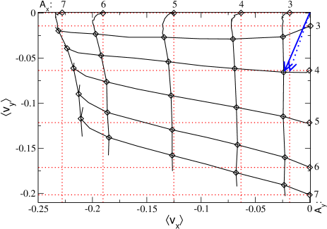
Figure 4: (Color online) Same as in Fig. 3 but for $\omega_{1}=\sqrt{2}$ and $\omega_{2}=1.41$, showing a considerably reduced lattice deformation. Note that the difference here between $\omega_{1}$ and $\omega_{2}$ is less than 0.3%.

If we intend to produce a current in a direction other than along the axes, we need to simultaneously apply drivings in both $x$ and $y$ directions. Fig. 3 shows what happens when this is done. The ideal situation for direction control would be that a superposition principle would apply, so that a specific required current direction could be obtained by applying the corresponding driving amplitudes in each perpendicular direction. However, Fig. 3 shows a very large deviation from this behavior, with the directed current values (solid lines and diamonds at the crossing between the lines) going far away from the ideal case (dotted lines). Looking for example at the current produced at $(A_{x},A_{y})=(3,4)$, one would expect, after observing the corresponding values at Fig. 2 (which are indicated in Fig. 3 with dotted lines), that a current is formed along the direction indicated in Fig. 3 by the dotted arrow. However, the current ends up having the direction given by the solid arrow, which forms a much larger angle with the $y$ axis than expected. In addition, further increasing $A_{y}$ additionally produces an unexpected non-monotonous behavior in $\langle v_{x}\rangle$, which makes control of the current direction rather difficult.

This phenomenon is due to the strong coupling between the $x$ and $y$ components at the same driving frequencies $\omega_{1}=\omega_{2}$. Remarkably, we can significantly suppress this coupling by using two incommensurate frequencies, as shown in Fig. 4. Note that the difference in $\omega_{2}$ with the case of periodic driving shown in Fig. 2 is just less than 0.3%, which implies that the curve shown in the top panel of this figure is practically indistinguishable from the one obtained with the latter frequency $\omega_{2}=1.41$. Fig. 4 shows that the deviation from an ideal behavior of uncoupled $x$ and $y$ dynamics is significantly reduced, in particular for weak driving [$A_{x,y}\leq 5$]. The deviation from such an ideal behavior is still pronounced at larger driving fields, with driving amplitude values close to the minima shown in Fig. 2.

A similar behavior is observed for a system with the following potential

$$U({\bf r})=U_{0}\left[\cos(kx)+2\cos(kx/2)\cos(\sqrt{3}y/2)\right],$$ (8)

which produces an hexagonal lattice in the XY plane, being in addition spatially symmetric in both perpendicular directions. Fig. 5 shows that the decoupling produced by the quasiperiodic driving is almost perfect for small driving amplitudes, allowing a precise control of the current direction.

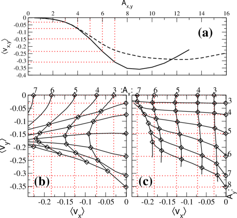
Figure 5: (Color online) Simulation results for the hexagonal potential (8) and the bidimensional driving (4) with $\omega_{1}=\sqrt{2}$ and: (b) $\omega_{2}=\sqrt{2}$ (periodic driving) and (c) $\omega_{2}=1.41$ (quasiperiodic driving). (a) shows the 1D current, when the biharmonic driving is applied in one direction only ($x$: solid line and $y$: dashed line), as a function of the amplitude the driving in the relevant direction.

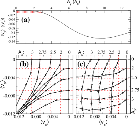
Figure 6: (Color online) Simulation results for the square potential of Eq. (9) and the bidimensional driving of Eq. (4) with $\omega_{1}=\sqrt{2}$ and: (b) $\omega_{2}=\sqrt{2}$ (periodic driving) and (c) $\omega_{2}=1.41$ (quasiperiodic driving). (a) shows the 1D current when the biharmonic driving is applied in one direction only as a function of the amplitude the driving in the relevant direction. In (b) and (c) the simulation data is represented by diamonds, with the solid lines being a guide to the eye connecting the data points. Each data point is estimated to have an error bar of about $\Delta v=0.001$ in each perpendicular direction (not drawn for clarity).

We have also studied a square lattice. Figure 6 shows the simulation results for the potential

$$U({\bf r})=U_{0}\cos(kx)\cos(ky).$$ (9)

Due to the explicit symmetry in the potential between the $x$ and $y$ directions, the directed current displays the strongest couplings when the biharmonic driving (4) is applied in both directions. The coupling is so strong that no significant improvement is found even with the quasiperiodic driving for moderate values of the driving amplitudes. Only at very small driving amplitudes – the values indicated in Fig. 6a with dotted lines – the quasiperiodic driving is able to diminish the couplings so that a reasonable control of the current direction is possible. Note that the current values shown in Fig. 6a and 6b are very small, and the simulation error bars are thus of considerable size. Still, it can be observed that the quasiperiodic driving is able to reduce significantly the large lattice distortion produced by the couplings.

In fact, we prove in the Appendix that this is a general result applicable to any spatially periodic system that is also spatially symmetric in both the $x$ and $y$ directions. A functional expansion in the driving amplitudes shows that the directed current of a system driven by the forces (4) with $\omega_{2}/\omega_{1}$ irrational is, in the first orders in the driving amplitudes $A_{x}$ and $A_{y}$,

$$\langle v_{x}\rangle=A_{x}^{3}B_{x0}\cos(\phi_{1}-\phi_{x0})+\mathcal{O}(5),$$ (10a)

$$\langle v_{y}\rangle=A_{y}^{3}B_{y0}\cos(\phi_{2}-\phi_{y0})+\mathcal{O}(5),$$ (10b)

where $B_{x0}$ ($B_{y0}$) and $\phi_{x0}$ ($\phi_{y0}$) are independent of the driving parameters $A_{x}$, $A_{y}$, $\phi_{1}$, $\phi_{2}$, and $\omega_{2}$ ($\omega_{1}$). Explicit expressions for the fifth order terms are given in the appendix. Therefore, in the lowest order on the driving amplitudes ($A_{x}^{3}$ for $\langle v_{x}\rangle$ and $A_{y}^{3}$ for $\langle v_{y}\rangle$), the current contains no coupling between the $x$ and $y$ directions when the quasiperiodic driving is applied. In contrast, with the periodic driving $\omega_{1}=\omega_{2}$, the current contains additional third order terms such as $A_{x}A_{y}^{2}$ in $\langle v_{x}\rangle$ and $A_{y}A_{x}^{2}$ in $\langle v_{y}\rangle$ (see the appendix), which makes the control of the current direction rather difficult for any values of the driving amplitudes. These considerations are not restricted to the specific equation of motion (1), since the calculations rely only on general symmetry considerations.

The observed partial loss of control at large driving amplitudes can also be explained within the framework of Dynamical Systems theory dynsys1 ; dynsys2 . The robustness of a quasiperiodic state can be understood by considering the two phases $\psi_{1}$, $\psi_{2}$ as coupled dynsys1 . We refer to the exactly solvable model

$$\dot{\psi}_{1}=\omega_{1}+f_{1}(\psi_{1},\psi_{2}),\quad\dot{\psi}_{2}=\omega_{2}+f_{2}(\psi_{1},\psi_{2}),$$ (11)

with $\omega_{1}$, $\omega_{2}$ incommensurate frequencies, and $f_{1}$ and $f_{2}$ arbitrary coupling functions that are $2\pi$-periodic in each argument. This model is useful to highlight the loss of quasiperiodicity in the dynamics at large driving amplitudes which, in our system, leads to loss of control. The key observation is the dependence of the commensurability of the observed frequencies $\Omega_{1}=\langle\dot{\psi}_{1}\rangle$ and $\Omega_{1}=\langle\dot{\psi}_{2}\rangle$ on the coupling functions. It is known that for small coupling $f_{1,2}$, the measure of all parameter values for which periodic regimes (i.e. $\Omega_{1}$ and $\Omega_{2}$ commensurate) are observed is small, while the measure of the corresponding quasiperiodic states is large. For large $f_{1,2}$, the measure of the periodic regimes grows, while that of quasiperiodic regimes decreases. These features are in agreement with the observed behavior in the 2D driven systems studied here.

V Conclusions

In conclusion, in this work we consider the problem of the control of transport in higher dimensional periodic structures by applied ac fields. In a generic lattice, transverse degrees of freedom are coupled, and this makes the control of motion difficult to implement. We show, both with a numerical and a rather general analytical analysis, that the use of quasiperiodic driving significantly suppresses the coupling between transverse degrees of freedom. Remarkably, this requires tiny variations of the frequency of the control field, of the order of few parts per thousand for the case studies presented in this work. The specific minimum variation required for quasiperiodic behavior in a real experiment or simulation is shown to depend on the observation time, as expected.

The dynamical decoupling of degrees of freedom allows a precise control of the transport, and does not require a detailed knowledge of the crystal geometry. Our results are of relevance for the control of transport in higher dimensional systems in which direct control, or knowledge, of the substrate geometry is lacking, as usually encountered in solid state systems vortex .

Appendix A Functional expansion in the driving amplitudes

We follow here the powerful method presented in Ref. quicue10 for a one-dimensional spatially periodic and symmetric system subject to the driving force

$$F(t)=A[\cos(p\omega t+\varphi_{1})+\cos(q\omega t+\varphi_{2})],$$ (12)

where $p$ and $q$ are positive integers. The current $\langle v\rangle=v[F]$ has a functional dependence on $F(t)$, and thus, it can be Taylor expanded as

$$v[F] = \sum_{n\geq 0}v_{n}[F],$$

$$v_{n}[F] = \{c_{n}(t_{1},\ldots,t_{n})F(t_{1})\cdots F(t_{n})\},$$ (13)

where

$$\{f(t_{1},\ldots,t_{n})\}\equiv\frac{1}{T^{n}}\int_{0}^{T}dt_{1}\cdots\int_{0}^{T}dt_{n}\,f(t_{1},\ldots,t_{n}),$$ (14)

$T$ is the period of the driving, and $c_{n}$ functions that can be chosen totally symmetric under any exchange of their arguments. It is shown in quicue10 that, when the system symmetries are taken into account, all terms in (A) with $n<p+q$ vanish, giving the lowest order possible contribution at $n=p+q$. Therefore, in the quasiperiodic limit, defined as $p,q\rightarrow\infty$ and $\omega\rightarrow 0$, so that $q\omega=\omega_{1},p\omega=\omega_{2}$, with $\omega_{1}$ and $\omega_{2}$ two incommensurate (finite) frequencies, all terms in (A) vanish, producing the expected suppression of current.

We can apply this method to a 2D system by using the expansion (A) for any component of the current, and then further Taylor expanding $c_{n}$ on the other component of the driving force. We then obtain for the $x$ component $\langle v_{x}\rangle=v_{x}[{\bf F}]$,

$$v_{x}[{\bf F}] = \sum_{n_{x}\geq 1}v_{n_{x},0}^{(x)}[F_{x},0]+\sum_{n_{x}n_{y}\geq 1}v_{n_{x},n_{y}}^{(x)}[{\bf F}],$$ (15a)

$$v_{n_{x},n_{y}}^{(x)}[{\bf F}] = \{c_{n_{x},n_{y}}(t_{1},\ldots,t_{n_{x}};t^{\prime}_{1},\ldots,t^{\prime}_{n_{y}})$$

$$\times F_{x}(t_{1})\cdots F_{x}(t_{n_{x}})F_{y}(t^{\prime}_{1})\cdots F_{y}(t^{\prime}_{n_{y}})\},$$

where we have already used the fact that $v_{x}[0,F_{y}]=0$ because of the system symmetries (see Eq. (18a)), and thus excluded the possibility $n_{x}=0$ from (15a). The first sum in the right-hand side of (15a) contains the terms which are independent of the transverse driving component $F_{y}(t)$, while the second sum accounts for the transverse couplings.

Before continuing, let us state explicitly the basic symmetries that we are going to use in the calculation. First, the potential $U(x,y)$ must be spatially symmetric in both directions, i.e. for each $y$ ($x$), there must exist a $x_{0}$ ($y_{0}$) such as

$$U(x_{0}+x,y)=U(x_{0}-x,y)\mbox{ for all }x,$$ (16a)

$$U(x,y_{0}+y)=U(x,y_{0}-y)\mbox{ for all }y.$$ (16b)

In this situation, the current can only appear by the application of a symmetry-breaking driving force, which thus controls the sign of the current

$$v_{x}[-F_{x},-F_{y}]=-v_{x}[F_{x},F_{y}],$$ (17a)

$$v_{y}[-F_{x},-F_{y}]=-v_{y}[F_{x},F_{y}],$$ (17b)

and for each component,

$$v_{x}[-F_{x},F_{y}]=-v_{x}[F_{x},F_{y}],$$ (18a)

$$v_{y}[F_{x},-F_{y}]=-v_{y}[F_{x},F_{y}].$$ (18b)

To satisfy the condition (17a), the functions $c_{n_{x},n_{y}}$ in (15) have to be identically zero for even values of $n=n_{x}+n_{y}$. Similarly, (18a) implies no contribution in (15) from terms with even values of $n_{x}$. In addition, in dissipative systems, as the one considered here, the current usually does not depend on the specific choice of time origin,

$$v_{x}[{\bf F}(t+t_{0})] = v_{x}[{\bf F}(t)],$$ (19a)

$$v_{y}[{\bf F}(t+t_{0})] = v_{y}[{\bf F}(t)],$$ (19b)

for any $t_{0}$. In non-dissipative systems displaying a strong dependence on the initial conditions, as in Hamiltonian ratchets reimann02 , the condition (19) can generally be satisfied either by averaging over the initial time flayev00 , or by adiabatically switching on the driving ${\bf F}(t)$. The implications of (19) depend on the explicit form of the driving force. Instead of (4), let us consider the following – slightly more general – biharmonic driving

$$F_{x}(t) = A_{x}[\cos(\omega_{1}t+\hat{\phi}_{1})+\cos(2\omega_{1}t+\phi_{1})],$$ (20a)

$$F_{y}(t) = A_{y}[\cos(\omega_{2}t+\hat{\phi}_{2})+\cos(2\omega_{2}t+\phi_{2})],$$ (20b)

where $\hat{\phi}_{1}$ and $\hat{\phi}_{2}$ are new driving phase constants. The conditions (19) imply that the current must be invariant under the following transformation

$$\hat{\phi}_{1}\rightarrow\hat{\phi}_{1}+\omega_{1}t_{0},\quad\phi_{1}\rightarrow\phi_{1}+2\omega_{1}t_{0},$$

$$\hat{\phi}_{2}\rightarrow\hat{\phi}_{2}+\omega_{2}t_{0},\quad\phi_{2}\rightarrow\phi_{2}+2\omega_{2}t_{0},$$ (21)

for any arbitrary $t_{0}$.

Expanding the cosines in (20) in complex exponentials yields

$$v_{n_{x},n_{y}}^{(x)}[{\bf F}]=\sum_{{\bf n}\geq 0}^{\otimes}A_{x}^{n_{x}}A_{y}^{n_{y}}C({\bf n})e^{i\Theta({\bf n},{\boldsymbol{\phi}})},$$ (22)

where ${\bf n}=(n_{1},n_{2},n_{3},n_{4},n_{1}^{\prime},n_{2}^{\prime},n_{3}^{\prime},n_{4}^{\prime})$, the symbol $\otimes$ denotes a restriction in the sum to the values of the tuple ${\bf n}$ such that

$$n_{1}+n_{2}+n_{3}+n_{4}=n_{x},$$

$$n^{\prime}_{1}+n^{\prime}_{2}+n^{\prime}_{3}+n^{\prime}_{4}=n_{y},$$ (23)

${\bf n}\geq 0$ denotes a component-wise inequality,

$${\boldsymbol{\phi}}=(\hat{\phi}_{1},\phi_{1},\hat{\phi}_{2},\phi_{2}),$$ (24)

and

$$\Theta({\bf n},{\boldsymbol{\phi}}) = [(n_{1}-n_{2})\hat{\phi}_{1}+(n_{3}-n_{4})\phi_{1}$$ (25)

$$+(n_{1}^{\prime}-n_{2}^{\prime})\hat{\phi}_{2}+(n_{3}^{\prime}-n_{4}^{\prime})\phi_{2}].$$

$C$ is a complex function of ${\bf n}$, $\omega_{1}$ and $\omega_{2}$ that can be traced back to time integrals of $c_{n_{x},n_{y}}$ multiplied by the factors $e^{\pm i\omega_{1}t_{k}}$ and $e^{\pm i\omega_{2}t_{k}^{\prime}}$. Further, it satisfies $C(\hat{\bf n})=C({\bf n})^{\ast}$, where $\ast$ denotes complex conjugate, and

$$\hat{\bf n}=(n_{2},n_{1},n_{4},n_{3},n^{\prime}_{2},n^{\prime}_{1},n^{\prime}_{4},n^{\prime}_{3}).$$ (26)

Thus, for every term in (22) with tuple ${\bf n}$, there is another term given by $\hat{\bf n}$ which is just the complex conjugate of the former, guaranteeing that $v_{n_{x},n_{y}}^{(x)}[{\bf F}]$ is real.

From Eq. (22), it is clear that the order of $v_{n_{x},n_{y}}^{(x)}[{\bf F}]$ is given by the factor $A_{x}^{n_{x}}A_{y}^{n_{y}}$, and thus by $n=n_{x}+n_{y}$.

Notice that the transformation (A) only affects $\Theta$ in (22). More specifically, it implies

$$(n_{1}-n_{2})+2(n_{3}-n_{4})+\frac{\omega_{2}}{\omega_{1}}\left[(n^{\prime}_{1}-n^{\prime}_{2})+2(n^{\prime}_{3}-n^{\prime}_{4})\right]=0.$$ (27)

Since $\omega_{2}/\omega_{1}$ is an irrational number, Eq. (27) is only satisfied when

$$(n_{1}-n_{2})+2(n_{3}-n_{4})=0,$$

$$(n^{\prime}_{1}-n^{\prime}_{2})+2(n^{\prime}_{3}-n^{\prime}_{4})=0.$$ (28)

The restrictions (A), together with (A) and the above mentioned conditions in $n_{x}$ and $n$ given by (17a) and (18a), determine the possible terms in the expansion (15a).

The lowest level in the expansion satisfying the above conditions is given by $v_{3,0}^{(x)}[F_{x},0]$, which is obviously independent of $F_{y}(t)$, having a contribution coming from the tuple ${\bf n}=(2,0,0,1,0,0,0,0)$ (and its corresponding complex conjugate $\hat{\bf n}$), and thus

$$v_{3,0}^{(x)}[F_{x},0]=A_{x}^{3}B_{x0}\cos(\phi_{1}-2\hat{\phi}_{1}-\phi_{x0}),$$ (29)

where $B_{x0}$ and $\phi_{x0}$ depend on the driving parameters only through $\omega_{1}$. This is the only third order term satisfying (A). All fourth order terms are forbidden due to the symmetry (17a). In the fifth order, there is one term containing no transverse coupling, $v_{5,0}^{(x)}$, coming from the tuples ${\bf n}=(2,0,1,2,0,0,0,0)$ and $(3,1,0,1,0,0,0,0)$. Then,

$$v_{5,0}^{(x)}[F_{x},0] = A_{x}^{5}[B_{x1}\cos(\phi_{1}-2\hat{\phi_{1}}-\phi_{x1})$$ (30)

$$+B_{x2}\cos(\phi_{1}-2\hat{\phi_{1}}-\phi_{x2})],$$

where $B_{xj}$ and $\phi_{xj}$, with $j=1,2$, depend on $\omega_{1}$ only. In this order, the only surviving coupling term is given by $v_{3,2}^{(x)}$, which has contributions from the tuples ${\bf n}=(2,0,0,1,1,1,0,0)$ and $(2,0,0,1,0,0,1,1)$, yielding

$$v_{3,2}^{(x)}[F_{x},F_{y}] = A_{x}^{3}A_{y}^{2}[B^{\prime}_{x1}\cos(\phi_{1}-2\hat{\phi_{1}}-\phi^{\prime}_{x1})$$ (31)

$$+B^{\prime}_{x2}\cos(\phi_{1}-2\hat{\phi_{1}}-\phi^{\prime}_{x2})],$$

where now $B^{\prime}_{xj}$ and $\phi^{\prime}_{xj}$ depend on $\omega_{1}$ and $\omega_{2}$.

Finally, note that when the ratio $\omega_{2}/\omega_{1}$ is rational (the case of periodic driving) there are additional terms that satisfy (27). More specifically, for $\omega_{1}=\omega_{2}$ the coupling term $v_{1,2}^{(x)}$ gives a non-vanishing contribution from the tuples ${\bf n}=(1,0,0,0,1,0,0,1)$ and $(0,0,0,1,2,0,0,0)$,

$$v_{1,2}^{(x)}[F_{x},F_{y}] = A_{x}A_{y}^{2}[B_{x1}^{p}\cos(\phi_{2}-\hat{\phi_{1}}-\hat{\phi_{2}}-\phi_{x1}^{p})$$ (32)

$$+B_{x2}^{p}\cos(\phi_{1}-2\hat{\phi_{2}}-\phi_{x2}^{p})].$$

References

- (1) P. Reimann, Phys. Rep. 361, 57 (2002).
- (2) P. Hänggi and F. Marchesoni, Rev. Mod. Phys. 81, 387 (2009).
- (3) V. Lebedev and F. Renzoni, Phys. Rev. A 80, 023422 (2009).
- (4) F. Marchesoni, Phys. Lett. A 119, 221 (1986).
- (5) D.R. Chialvo and M.M. Millonas, Phys. Lett. A 209, 26 (1995).
- (6) M.I. Dykman, H. Rabitz, V.N. Smelyanskiy, and B.E. Vugmeister, Phys. Rev. Lett. 79, 1178 (1997).
- (7) S. Flach, O. Yevtushenko, and Y. Zolotaryuk, Phys. Rev. Lett. 84, 2358 (2000).
- (8) L. Machura, M. Kostur, and J. Luczka, Chem. Phys. 373 (2010).
- (9) D. Cubero, V. Lebedev, and F. Renzoni, Phys. Rev. E 82, 041116 (2010).
- (10) A. Wickenbrock, D. Cubero, N. A. Abdul Wahab, P. Phoonthong, and F. Renzoni, Phys. Rev. E 84, 021127 (2011).
- (11) S. Denisov, Y. Zolotaryuk, S. Flach, and O. Yevtushenko, Phys. Rev. Lett. 100, 224102 (2008).
- (12) E. Neumann and A. Pikovsky, Eur. Phys. J. B 26, 219 (2002).
- (13) V.I. Arnold, Mathematical Methods of Classical Mechanics, Springer, New York (1989).
- (14) S. Flach and S.Denisov, Acta Phys. Pol. B 35, 1437, 2004.
- (15) R. Gommers, S. Denisov, and F. Renzoni, Phys. Rev. Lett. 96,240604 (2006).
- (16) R. Gommers, M. Brown, and F. Renzoni, Phys. Rev. A 75, 053406 (2007).
- (17) N.R. Quintero, J.A. Cuesta, and R. Alvarez-Nodarse, Phys. Rev. E 81, 030102R (2010).
- (18) A. Katok and B. Hasselbatt, Introduction to the modern theory of dynamical systems, Cambdrige University Press, 1995.
- (19) U. Feudel, S. Kuznetsov, and A. Pikovsky, Strange nonchaotic attractors, dynamics between order and chaos in quasiperiodically forced systems, World Sicentific Publishing Co., Singapure, 2006.
- (20) D.E. Shalóm and H. Pastoriza, Phys. Rev. Lett. 94, 177001 (2005); S. Savel’ev and F. Nori, Nat. Mater. 1, 179 (2002); D. Cole et al., Nat. Mater. 5, 305 (2006); S. Ooi et al, Phys. Rev. Lett. 99, 207003 (2007).