Numerical study of broadband spectra caused by internal shocks in magnetized relativistic jets of blazars.

Abstract

The internal-shocks scenario in relativistic jets has been used to explain the variability of blazars’ outflow emission. Recent simulations have shown that the magnetic field alters the dynamics of these shocks producing a whole zoo of spectral energy density patterns. However, the role played by magnetization in such high-energy emission is still not entirely understood. With the aid of Fermi’s second LAT AGN catalog, a comparison with observations in the $\gamma$-ray band was performed, in order to identify the effects of the magnetic field.

1 Introduction

Relativistic outflows have been observed extensively in blazars, a class of radio-loud active galactic nuclei (AGNs) whose jets are pointing very close to the line of sight towards the observer Urry:1995aa , and known for showing the most rapid variability of all AGNs. Their remarkable characteristic flares in the X-ray frequency range usually have a duration of the order of one day. Often the internal-shocks (IS) scenario Rees:1994ca is invoked to explain this variability Spada:2001do ; Mimica:2004ay ; Mimica:2005aa . The IS scenario is an idealized model of a variable jet where an intermittently working central engine ejects shells of magnetized plasma which collide due to their velocity differences. As a consequence of the collision internal shocks are formed, particles are accelerated at the shock fronts and the non-thermal, highly variable radiation is produced.

Our long-term project is the study of the influence of magnetic fields on the radiation from IS using numerical simulations. In Mimica:2012aa we studied a large number of shell collisions with different magnetization levels. In the present work we focus on a limited number of shell magnetization levels, but vary other parameters such as the jet viewing angle, bulk Lorentz factor of the shells, and their relative Lorentz factor. The data obtained from these simulations is used to categorize the specific effects that variations of each parameter have on average spectra. These synthetic observations are then compared with the second LAT AGN catalog (2LAC) of blazars observed by Fermi Ackermann:2011apj .

Our numerical setup is describen in Sec. 2. The results are shown in Sec. 3. Finally we discuss briefly our results in Sec. 4.

2 Numerical Setup

We use a modified version of the SPEV codeMimica:2009aa ; Mimica:2012aa to compute the non-thermal emission from the IS. We do not consider the full hydrodynamic interaction of colliding magnetized shells (see. e.g. Mimica:2007aa for a detailed study). Instead, we simplify the shell interaction as a one-dimensional Riemann problem and focus our resources on a more detailed treatment of the non-thermal radiation. Our method consists of three phases:

1. Solution of the Riemann problem. Making use of an exact RMHD Riemann solver Romero:2005zr we determine the properties of the internal shock waves. We follow the procedure described in Mimica:2010aa to set-up the shells and to extract the information needed for the steps 2 and 3.

2. Non-thermal particles transport and evolution. The particles are injected behind the shock fronts following the prescription of Bottcher:2010gn ; Joshi:2011bp ; Mimica:2012aa . We assume that a fraction of the thermal electrons are accelerated to high energies, and that their energy density is a fraction of the internal energy density of the shocked fluid. We assume a cylindrical shell geometry and perform all the calculations in the rest frame of the shocked fluid. In this frame the shocks are propagating away from the initial discontinuity, injecting and leaving non-thermal particles behind. We evolve the energy distribution of non-thermal electrons taking into account synchrotron and inverse-Compton (IC) losses. See Mimica:2012aa for more details.

3. Radiative transfer. The total emissivity at each point is assumed to be a combination of the following emission processes: (1) synchrotron radiation, (2) IC upscattering of an external radiation field (EIC) and (3) synchrotron self-Compton (SSC). The details of how they are calculated are given in Mimica:2012aa . The radiative transfer equation is solved taking into account the relativistic effects and time delays.

We compute light curves and average spectral energy distribution (SED) for each shell collision. In this work we focus our attention on how parameter variations affect the SEDs.

3 Results

As mentioned in Sec. 1, the aim of this work is to cover a wider range in the parameter space than was done in Mimica:2012aa . We group our models according to the initial shell magnetization, $\sigma:=B^{2}/4\pi\rho\Gamma^{2}c^{2}$. We denote by letters S, M and W the following families of models:

• weakly magnetized, $\sigma_{L}=10^{-6},\sigma_{R}=10^{-6}$,

• moderately magnetized, $\sigma_{L}=10^{-2},\sigma_{R}=10^{-2}$, and

• strongly magnetized, $\sigma_{L}=1,\sigma_{R}=10^{-1}$.

Hereafter the subscripts $L$ and $R$ will denote left (faster) and right (slower) shells, respectively. As parameters to vary we considered both intrinsic and extrinsic ones. Among the intrinsic parameters we choose the Lorentz factor of the slow shell, $\Gamma_{R}$, and the relative Lorentz factor $\Delta g:=\Gamma_{L}/\Gamma_{R}-1$, where $\Gamma_{L}$ is the Lorentz factor of the fast shell. The parameter space covered is shown in Table 1.

Parameter	value
$\sigma_{L}$	$10^{-6},\ 10^{-2},\ 1$
$\sigma_{R}$	$10^{-6},\ 10^{-2},\ 10^{-1}$
$\Gamma_{R}$	$10,12,17,20,22,25$
$\Delta g$	$0.5,0.7,1.0,1.5,2.0$
$\theta$	$5$

Table 1: Parameters of the models. $\Gamma_{R}$ is the Lorentz factor of the slow shell, $\sigma_{L}$ and $\sigma_{R}$ are the fast and slow shell magnetizations and $\theta$ is viewing angle of the observer.

For clarity, when we refer to a particular model we label it by appending the values of each of these parameters to the model letter. For instance, S-G10-D1.0-T5 is the strongly magnetized model with $\Gamma_{R}=10$ (G10), $\Delta g=1.0$ (D1.0) and $\theta=5^{\circ}$ (T5). If we refer to a subset of models with one or two parameters fixed we use an abbreviated notation, where we omit the varying parameters from the label. We compute the spectra for a typical source located at $z=0.5$.

In the rest of this section we will present some of the final SEDs resulting from our simulations. A larger collection is shown in (Rueda:2013aa, ). The SEDs of each model has been averaged over the time interval $0-10^{6}$ s.

3.1 Weakly-magnetized models

The SEDs computed for the models W-G10-T5 (varying $\Delta g$) are shown in the left panel of Fig. 1. The spectra show that with increasing $\Delta g$ the IC component also increases, up to three orders of magnitude. In order to see the effects on each emission process, the synchrotron, SSC and EC components for $\Delta g=0.5,2.0$ are shown as dashed, dot-dashed and dot-dot-dashed lines, respectively. As we can see, while the three components of the spectrum (synchrotron, SSC and EC) are around the same order of magnitude for $\Delta g=0.5$, for $\Delta g=2.0$ the SSC is almost two orders of magnitude more luminous than the other two. The inset shows the $\gamma$-ray spectral slope of each model as a function of its $\gamma$-ray flux (see Sec. 3.4).

3.2 Moderately-magnetized models

The SEDs of the family of models M-D1.0-T5 are presented in the right panel of Fig. 1. Analogous to the left panel of Fig. 1 the synchrotron, SSC and EC components are shown as dashed, dot-dashed and dot-dot-dashed lines, respectively, for $\Gamma_{R}=10,17,25$. The synchrotron component for $\Gamma_{R}=10$ is $\simeq 20$ times brighter than the SSC one, in contrast to the EC which is $100$ times dimmer. For $\Gamma_{R}=25$ the EC is of the same order of magnitude of SSC and synchrotron. The latter two decrease one order of magnitude between M-G10-D1.0-T5 and M-G25-D1.0-T5, while the EC grows by almost one order of magnitude. This is a consequence of the fact that the number of electrons and the comoving magnetic field strength decrease with the increasing $\Gamma_{R}$ Mimica:2012aa , which means that there are less synchrotron photons and less electrons which can scatter them in the SSC process. On the other hand, the radiation field density of the seed photons for the EC is independent of $\Gamma_{R}$, which, in combination with the Doppler boost causes the increase in the EC luminosity. We also see that at $\simeq 10^{23}$ Hz there is a point where all the EC spectra coincide. This is due to the Klein-Nishina cutoff, which we model as a sharp cutoff. The inset shows that the there is no significant change in the flux of $\gamma$-ray photons, although there was for the spectral index, heading towards lower values for increasing $\Gamma_{R}$.

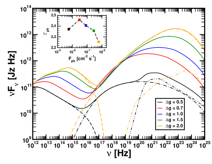
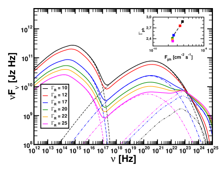
Figure 1: Left panel: Averaged spectra resulting from the collision of weakly magnetized shells ($\sigma_{L}=\sigma_{R}=10^{-6}$). For the models $\Delta g=0.5,2.0$, the synchrotron, SSC and EIC contributions (dashed, dot-dashed and dot-dot-dashed lines, respectively) are shown. The inset shows the photon spectral slope $\Gamma_{ph}$ as a function of the photon flux $F_{ph}$ in the $\gamma$-ray band (see Sec. 3.4). Colors of the points correspond to the line colors in the main plot. Right panel: Same as the left panel, but for moderately magnetized shells ($\sigma_{L}=\sigma_{R}=10^{-2}$) and varying $\Gamma_{R}$. For models with $\Gamma_{R}=10,17,25$ we plot the synchrotron, SSC and EIC contributions.

3.3 Strongly-magnetized models

The third model family consists of the strongly magnetized models where $\sigma_{L}=1$ and $\sigma_{R}=0.1$. The SEDs of the series of models S-D1.0-T5 appear in Fig. 2. As we can see, for $\Gamma_{R}=10$ the synchrotron component is $\simeq 100$ times brighter than the IC. For $\Gamma_{R}=25$ this difference decreases to one order of magnitude. The EIC component rises with rising $\Gamma_{R}$, to the point in which it begins to be comparable to the synchrotron component. These effects are similar to the family M-D1.0-T5, described in Sec. 3.2. The spectra converge due to our treatment of the Klein-Nishina cutoff. In the inset we can see that the flux of $\gamma$-ray photons does not change appreciably in this family of models.

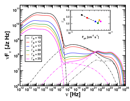
Figure 2: Same as right panel in Fig. 1, but for strongly magnetized shells ($\sigma_{L}=1,\sigma_{R}=$ 0.1).

3.4 $\gamma$-rays spectral slope

A linear mean-squares algorithm is used to deduce the $\gamma$-ray spectral slope $\Gamma_{ph}$. Due to the fact that we are not modeling the Klein-Nishina part of the spectrum, we only performed the calculations of $\Gamma_{ph}$ for those models that do not show a large drop-off in the photon flux. In Fig. 3 we show $\Gamma_{ph}$ as a function of the photon flux for energies $>0.2\,$GeV, where $F_{ph}$ is the photon flux for photon energies $>0.1$ GeV Abdo:2009cb . We compare our results with sources found in 2LAC catalogue Ackermann:2011apj (restricting the comparsion to sources with $0.4\leq z\leq 0.6$). In Fig. 3 we see that weakly and moderately magnetized models overlap with the observations, with more weakly than moderately magnetized models falling within the observed part of the parameter space.

Preliminary results of models where the viewing angle, $\theta$, is changed; i. e. SMW-G10-D1.0, appear also in Fig. 3.

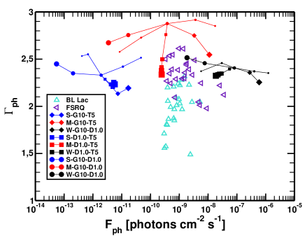
Figure 3: Spectral slope $\Gamma_{ph}$ as a function of the photon flux for energies $>100$ MeV. $\Gamma_{ph}$ is computed for the photon energies $>200$ MeV Abdo:2009cb . The symbols joined by lines represent our numerical models, while cyan and magenta triangles represent BL Lacs and FSRQs at redshift $z\simeq 0.5$ from 2LAC Ackermann:2011apj . In this figure we also show the preliminary three families of models where we vary the opening angle (filled circles).

4 Conclusions

In this paper we report on the progress of the study of the influence of the jet magnetization on blazar flares. We vary two parameters of our models: the relative Lorentz factor $\Delta g$ and the bulk Lorentz factor $\Gamma_{R}$.

When $\Delta g$ is increased we get a more luminous maximum of the inverse Compton component, which is dominated by the SSC. If $\Gamma_{R}$ is increased we find that the EIC begins to dominate over SSC, as well as becoming comparable to the synchrotron component. In the case of strongly magnetized shells, if $\Gamma_{R}\sim 50$ both synchrotron and EC components are of the same order of magnitude (see Rueda:2013aa ). Among all the models studied here, the weakly magnetized are the ones that best fit Fermi observations Ackermann:2011apj . However, the tendencies of certain models with higher magnetization appear to also be consistent with the observations.

References

- (1) C.M. Urry, P. Padovani, PASP 107, 803 (1995)
- (2) M.J. Rees, P. Meszaros, ApJL 430, L93 (1994)
- (3) M. Spada, G. Ghisellini, D. Lazzati, A. Celotti, MNRAS 325, 1559 (2001)
- (4) P. Mimica, M.A. Aloy, E. Müller, W. Brinkmann, A&A 418, 947 (2004)
- (5) P. Mimica, M.A. Aloy, E. Müller, W. Brinkmann, A&A 441, 103 (2005)
- (6) P. Mimica, M.A. Aloy, MNRAS 421, 2635 (2012)
- (7) M. Ackermann et al., ApJ 743, 171 (2011)
- (8) P. Mimica, M.A. Aloy, I. Agudo, J.M. Marti, J.L. Gómez, J.A. Miralles, ApJ 696, 1142 (2009)
- (9) P. Mimica, M.A. Aloy, E. Müller, A&A 466, 93 (2007)
- (10) R. Romero, J. Marti, J.A. Pons, J.M. Ibáñez, J.A. Miralles, JFM 544, 323 (2005)
- (11) P. Mimica, M.A. Aloy, MNRAS 401, 525 (2010)
- (12) M. Böttcher, C. Dermer, ApJ 711, 445 (2010)
- (13) M. Joshi, M. Böttcher, ApJ 727, 21 (2011)
- (14) J. Rueda-Becerril, P. Mimica, M.A. Aloy, MNRAS, in preparation (2013)
- (15) A.A. Abdo, M. Ackermann, M. Ajello, W.B. Atwood, M. Axelsson, L. Baldini, J. Ballet, B. et al., ApJ 700, 597 (2009), 0902.1559