Oscillatory regimes of the thermomagnetic instability in superconducting films

Abstract

The stability of superconducting films with respect to oscillatory precursor modes for thermomagnetic avalanches is investigated theoretically. The results for the onset threshold show that previous treatments of non-oscillatory modes have predicted much higher thresholds. Thus, in film superconductors, oscillatory modes are far more likely to cause thermomagnetic breakdown. This explains the experimental fact that flux avalanches in film superconductors can occur even at very small ramping rates of the applied magnetic field. Closed expressions for the threshold magnetic field and temperature, as well oscillation frequency, are derived for different regimes of the oscillatory thermomagnetic instability.

The irreversible electromagnetic properties of type-II superconductors are commonly explained in terms of the critical current density $j_{c}$, as introduced by Bean Bean (1964). In the corresponding critical state the distribution of magnetic flux is nonuniform and metastable. However, since $j_{c}$ is a decreasing function of temperature the metastable state can become unstable driven by the Joule heat generated during flux motion. In bulk superconductors this thermomagnetic instability gives rise to abrupt displacement of large amounts of flux, so-called flux jumps, which may cause the entire superconductor to be heated to the normal state Wipf (1967); Swartz and Bean (1968); Mints and Rakhmanov (1981); Wipf (1991); Rakhmanov et al. (2004). In some cases, pronounced oscillations in magnetization and temperature have been detected prior to such jumps Legrand et al. (1993); Mints (1996).

In film superconductors experiencing an increasing transverse magnetic fields, the thermomagnetic instability gives rise to abrupt flux entry in the form of dendritic structures rooted at the sample edge Wertheimer and J. le G. Gilchrist (1967). Using magneto-optical imaging Ch. Jooss et al. (2002) the residual flux distribution left in the film after such avalanche events have been observed in many superconducting materials Leiderer et al. (1993); Vlasko-Vlasov et al. (2000); Johansen et al. (2002); Welling et al. (2004). The experiments also show that there is a threshold magnetic field, $H_{\rm th}$, for the onset of avalanche activity, and that the unstable behavior is restricted to temperatures below a threshold value, $T_{\rm th}$, see Fig. 1. These thresholds have been explained on the basis of linear stability analysis of the nonlinear and non-local equations governing the electrodynamics of such films Mints and Brandt (1996); Aranson et al. (2005); Shantsev et al. (2005); Denisov et al. (2006a, b); Albrecht et al. (2007). The theoretical works show that in order to trigger avalanches an electrical field in the range $E=$ 30-100 mV/m is required.

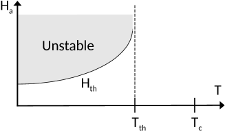
Figure 1: Generic thermomagnetic stability diagram of film superconductors.

Experimentally, one finds in films of many materials, e.g., MgB₂, Nb and NbN, that avalanches occur even when the magnetic field is ramped very slowly, e.g., below 1 mT/s Johansen et al. (2001), inducing correspondingly small $E$-fields. For a film placed in a magnetic field ramped at a rate of $\mu_{0}\dot{H}_{a}$ the Bean model estimates Brandt (1995) the $E$-field along the edge as $E\sim\mu_{0}\dot{H}_{a}w$, where $w$ is the half-width of the film. With a size of a few millimeters and a ramping rate of 1 mT/s the edge field is $E\sim 1~{}\mu$V/m, i.e., several orders of magnitude below the theoretical threshold. Hence, thermomagnetic avalanches should not occur at such ramping rates, quite contrary to experiment.

This inconsistency led to the suggestion Denisov et al. (2006b) that large local $E$-fields are created by non-thermomagnetic micro-avalanches, which in turn trigger the large and devastating Baziljevich et al. (2014) events. From a modelling viewpoint this idea poses severe challenges since the proposed micro-avalanche scenarios Field et al. (1995); Olson et al. (1997); Altshuler and Johansen (2004); Guillamón et al. (2011) have not yet allowed evaluation of the $E$-fields.

In the present work, earlier analyses of the onset conditions for thermomagnetic avalanches are generalized by including modes with complex instability increments. Thus, scenarios involving oscillatory precursor behavior are here considered. It is found that such modes, depending on the material parameters, can have much lower thresholds compared to those of the non-oscillatory ones. As a result, the thermomagnetic instability can develop directly from the low $E$-field background of the Bean critical state, without assuming existence of micro-avalanches of unspecified nature.

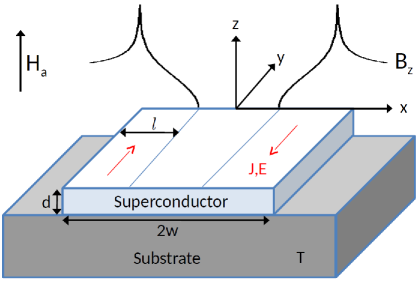
Figure 2: (Color online) Sample geometry: A long superconducting strip in thermal contact with a substrate and exposed to an increasing magnetic field $H_{a}$ applied along the $z$-axis, inducing currents and electrical fields in the $y$-direction.

Consider a superconducting film shaped as a strip of thickness $d$ and width $2w$, where $w\gg d$. The strip is very long in the $y$-direction, and is in thermal contact with the substrate, see Fig. 2. The sample is initially zero-field cooled to a temperature, $T$, below the superconducting transition temperature, $T_{c}$, whereupon a perpendicular magnetic field $H_{a}$ is applied at a constant rate $\dot{H}_{a}$. The overall flux dynamics in the superconductor is assumed to follow the Bean model. The magnetic flux then penetrates to a depth $l$, which increases with the field as Brandt and Indenbom (1993),

$$l/w=1-\cosh^{-1}(\pi H_{a}/dj_{c}).$$ (1)

This flux motion induces an electrical field, which is maximum at the strip edge where the value is given by Brandt (1995),

$$E_{\rm edge}=\mu_{0}\dot{H}_{a}w\tanh\left(\pi H_{a}/dj_{c}\right).$$ (2)

For perturbations of the Bean state, we describe the superconductor using the more general model Mints and Brandt (1996),

$$\mathbf{E}=\left\{\begin{array}[]{ll}\rho_{n}\left(J/dj_{c}\right)^{n-1}\mathbf{J}/d,&J<dj_{c}\mbox{ and below}~{}T_{c},\\ \rho_{n}\mathbf{J}/d,&\mbox{otherwise}.\end{array}\right.$$ (3)

Here, $\mathbf{J}$ is the sheet current, $\rho_{n}$ is the normal state resistivity, and $n$ is the flux creep exponent. The Bean model corresponds to the limit $n\to\infty$.

The electrodynamics follows the Maxwell equations

$$\dot{\mathbf{B}}=-\nabla\times\mathbf{E},~{}~{}\nabla\times\mathbf{H}=\mathbf{J}\delta(z),~{}~{}\nabla\cdot\mathbf{B}=0,$$ (4)

with $\nabla\cdot\mathbf{J}=0$, $\mu_{0}\mathbf{H}=\mathbf{B}$. The heat-flow in the strip is described by

$$c\dot{\tilde{T}}=\kappa\nabla^{2}{\tilde{T}}-\frac{h}{d}({\tilde{T}}-T)+\frac{1}{d}\mathbf{J}\cdot\mathbf{E}\,,$$ (5)

where ${\tilde{T}}$ is the local temperature in the superconductor, and $T$ is the uniform substrate temperature. The superconductor’s specific heat is $c$, its thermal conductivity is $\kappa$, and $h$ is the coefficient of heat transfer between the strip and the substrate. The temperature dependencies are chosen as $c=c_{0}({\tilde{T}}/T_{c})^{3}$, $\kappa=\kappa_{0}({\tilde{T}}/T_{c})^{3}$, and $h=h_{0}({\tilde{T}}/T_{c})^{3}$. For the electrodynamical parameters we use $j_{c}=j_{c0}(1-{\tilde{T}}/T_{c})$ and $n=n_{0}T_{c}/{\tilde{T}}$.

To determine the conditions for onset of oscillatory regimes of the instability, consider the threshold electric field, $E_{\rm th}$, following from linearization of Eqs. (3)–(5). As shown in Ref. J. I. Vestgården et al. (2013) this gives

$$\frac{j_{c}}{T^{*}}nE_{\rm th}-\kappa k^{2}-\frac{h}{d}-\frac{2}{k}\left(k_{x}^{2}+\frac{k_{y}^{2}}{n}\right)\frac{c}{\mu_{0}dj_{c}}nE_{\rm th}=0,$$ (6)

where $T^{*}=|\partial\ln j_{c}/\partial T|^{-1}$, and $k_{x}$, $k_{y}$ and $k=\sqrt{k_{x}^{2}+k_{y}^{2}}$ are the Fourier space wave-vectors. The instability onset is accompanied by temporal oscillations with frequency

$$\begin{split}\omega^{2}&=\frac{2}{k}\frac{nE_{\rm th}}{\mu_{0}dj_{c}c}\\ \times&\left[\left(k_{x}^{2}+\frac{k_{y}^{2}}{n}\right)\left(\kappa k^{2}+\frac{h}{d}\right)+\left(k_{x}^{2}-k_{y}^{2}\right)\frac{j_{c}E_{\text{th}}}{T^{*}}\right].\end{split}$$ (7)

As $H_{a}$ increases from zero, the most unstable modes correspond to $k_{y}=0$ and $k_{x}=\pi/2l$, and in what follows only these modes are considered.

First, at small $H_{a}$, the main mechanism for suppression of the instability is the lateral heat diffusion. Thus, neglecting in Eq. (6) the terms proportional to $c$ and $h$, one obtains

$$E_{{\rm th},\kappa}=\frac{\kappa T^{*}}{nj_{c}}\left(\frac{\pi}{2l}\right)^{2}.$$ (8)

For small $H_{a}$, the Eq. (1) gives $l\approx(w/2)(\pi H_{a}/dj_{c})^{2}$, and from Eq. (2) the electric field is $E_{\text{edge}}\approx\mu_{0}\dot{H}_{a}w\pi H_{a}/dj_{c}$. Inserting these expressions in Eq. (8) the threshold applied magnetic field becomes,

$$H_{{\rm th},\kappa}=\frac{dj_{c}}{\pi}\left(\frac{\pi^{2}\kappa T^{*}}{nw^{3}j_{c}\mu_{0}\dot{H}_{a}}\right)^{1/5}.$$ (9)

This formula gives the threshold field as a function of temperature through the parameters $\kappa$, $j_{c}$ and $n$. The corresponding oscillation frequency, obtained from Eq. (7) assuming $n\gg 1$, is

$$\omega_{\kappa}=\mu_{0}\dot{H}_{a}n\ \sqrt{\frac{2\pi w}{\mu_{0}dcT^{*}}}\,,$$ (10)

which depends on temperature through $n$, $c$ and $T^{*}$.

Then, at deeper penetration, when $l\gg(\pi/2)\sqrt{\kappa d/h}$, the main mechanism suppressing the instability is heat removal by the substrate. In this case one can in Eq. (6) ignore the terms proportional to $\kappa$ and $c$, which gives,

$$E_{{\rm th},h}=\frac{hT^{*}}{ndj_{c}}.$$ (11)

Combining this with Eq. (2) to eliminate the $E$-field one obtains the following threshold magnetic field

$$H_{{\rm th},h}=\frac{dj_{c}}{\pi}\operatorname{atanh}\left(\frac{hT^{*}}{nwdj_{c}\mu_{0}\dot{H}_{a}}\right).$$ (12)

Also this case is accompanied by oscillations, and at full penetration, when $E_{\rm edge}\approx\mu_{0}\dot{H}_{a}w$, the frequency is $\omega_{h}=\omega_{\kappa}/\sqrt{2}$. Thus, $\omega_{h}$ and $\omega_{\kappa}$ are not very different in magnitude, and they have a common temperature dependence.

From Eq. (12) it follows that $H_{{\rm th},h}$ diverges when the parameters satisfy the equality

$$hT^{*}/(nwdj_{c}\mu_{0}\dot{H}_{a})=1.$$

When the left hand side exceeds unity the instability will not occur, and it is therefore the condition determining the threshold temperature, $T_{\rm th}$. Thus, one finds

$$T_{\rm th}/T_{c}=(n_{0}wdj_{c0}\mu_{0}\dot{H}_{a}/T_{c}h_{0})^{1/4},$$ (13)

using the above temperature dependencies of $j_{c}$, $n$ and $h$.

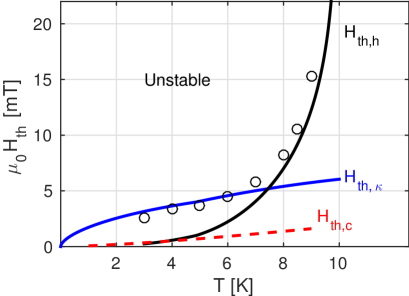
Figure 3: (Color online) Threshold magnetic fields $H_{{\rm th},\kappa}$ (blue), $H_{{\rm th},h}$ (black), and $H_{{\rm th},c}$ (dashed red), as functions of temperature. The discrete points represent the numerical results.

To verify the validity of the derived predictions near the instability onset the set of full equations (3) - (5) were solved numerically using the procedure described in Ref. Vestgården et al. (2011). Material parameters typical for MgB₂ films Vestgården et al. (2011); Thompson et al. (2005) were used, i.e., $T_{c}=39~{}$K, $c_{0}=35\cdot 10^{3}~{}$J/m, $\kappa_{0}=160~{}$W/Km³, $\rho_{n}=7\cdot 10^{-8}~{}\Omega$m, $j_{c0}=1\cdot 10^{11}$ Am^-2, and $n_{0}=50$. The creep exponent was limited to $n=400$ at low temperatures. The field ramp rate was set to $\mu_{0}\dot{H}_{a}=600$ mT/s, and the sample dimensions were $w=2$ mm and $d=0.5~{}\mu$m. The substrate cooling parameter, not known from measurements, was taken as $h_{0}=1.8\cdot 10^{4}~{}$W/Km² to give a threshold temperature near 10 K, in accordance with experimental observations Johansen et al. (2001). Numerical results were obtained for temperatures down to 3 K.

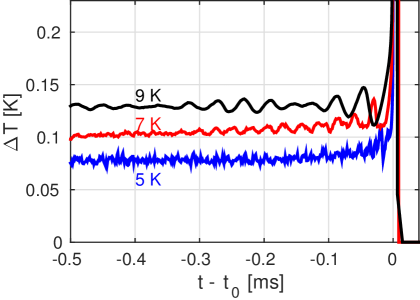
Figure 4: (Color online) Temporal variations in temperature prior to avalanches at 5, 7 and 9 K.

Figure 3 shows the threshold magnetic field as function of temperature. The full curves represent the analytical expressions $H_{{\rm th},\kappa}$ and $H_{{\rm th},h}$, while the discrete data show the simulation results. Each data point indicates the applied field when the first dendritic avalanche occurred as the field increased from zero. At $T=9.5$ K the simulations stopped generating avalanches. From the figure one sees that for $T<7$ K, the graph representing $H_{{\rm th},\kappa}$ fit the numerical data very well. From 7 K the data cross over to follow closely the curve representing $H_{{\rm th},h}$. The dashed curve represents the adiabatic threshold field, $H_{{\rm th},c}$, which clearly does not fit the simulations results at any temperature, see below for more discussion.

Direct evidence for oscillatory behavior preceding the onset of avalanches is presented in Fig. 4. The figure shows temporal fluctuations in the excess temperature, $\Delta T=\max\{\tilde{T}\}-T$, over an interval of 0.5 ms prior to avalanche events at $T=$ 5, 7 and 9 K. The $t_{0}$ is the time of avalanche onset, defined as when $\max\{\tilde{T}\}=T_{c}$. The graph obtained at 9 K shows in the whole time interval clear oscillations with one dominant frequency. During the last 0.1 ms before $t=t_{0}$ the amplitude is growing significantly. A quite similar behavior is evident also in the graph obtained at $T=7$ K. The oscillations are here smaller in amplitude, and noise is more pronounced. Nevertheless, nearly harmonic oscillations occur during the last 0.3 ms before onset, and their frequency is larger than at 9 K. As in the curve for 9 K the oscillation amplitude increases towards the onset. In addition, the dc-part of the $\Delta T$ signal also increases slightly towards time $t_{0}$. At 5 K, on the other hand, rapid fluctuations dominate the behavior, and a characteristic frequency is not present. The dc-part of $\Delta T$ increases also here when approaching the time of onset.

The characteristic frequency, $\omega$, found from the simulation results at temperatures between 6 K and 9 K is plotted as discrete data in Fig. 5. The $\omega$ was obtained from the location of the peak in the Fourier spectrum of $\Delta T(t)$, prior to the first avalanche occurring at each temperature. The full curves in the figure represent the analytical expressions $\omega_{\kappa}$ and $\omega_{h}$. One sees that the decrease in $\omega$ with increasing temperature is following the curves for $\omega_{h}(T)$ and $\omega_{\kappa}(T)$ very well.

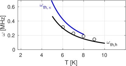
Figure 5: (Color online) Oscillation frequency as function of temperature. The discrete data represent the numerical results, while the full curves are from theory.

Regarding the adiabatic condition, i.e., when the instability is prevented only by the heat capacity of the superconductor, the threshold field follows from Eq. (6) with $\kappa=h=0$. Using $k_{x}$ with $l(H_{a})$ from Eq. (1) in the shallow penetration limit, one finds

$$H_{{\rm th},c}=\sqrt{\frac{2}{\pi}\frac{cT^{*}}{\mu_{0}}\frac{d}{w}}\,.$$ (14)

This expression was obtained previously Shantsev et al. (2005); Denisov et al. (2006a). New here is that also this threshold is associated with oscillations, and the frequency is contained in Eq. (7). However, for the material parameters and field ramp rate used in our simulations the frequency curve falls far outside the scale in Fig. 5, signalling that the adiabatic limit is in this case not relevant at any temperature. This is fully consistent also with the poor fit of the curve $H_{{\rm th},c}(T)$ to the numerical data in Fig. 3.

Finally, it is interesting to compare the onset thresholds obtained for the different oscillatory regimes with those from previous works, where only non-oscillatory modes were considered. In Ref. Denisov et al. (2006b), the following expression was obtained for the threshold electric field,

$$E_{\text{th}}=\frac{T^{*}}{j_{c}}\left(\frac{\pi}{2l}\sqrt{\kappa}+\sqrt{\frac{h}{nd}}\right)^{2}.$$ (15)

By direct comparison, it follows that this threshold is higher than the oscillatory thresholds derived in the present work. For example, in the case when $h=0$ the $E_{\text{th}}$ in Eq. (15) is a factor $n$ larger than $E_{{\rm th},\kappa}$ of Eq. (8). Thus, in an increasing applied magnetic field the onset condition for this oscillatory regime will be met long before that of the non-oscillatory instability.

In conclusion, several oscillatory regimes of the thermomagnetic instability in superconducting films were analysed and explicit onset conditions, i.e., threshold temperature, electric and applied magnetic field, were obtained as functions of material parameters and field ramping rate. The analytical work was supplemented by numerical simulations, and both confirm that oscillatory modes are more unstable than the conventional ones. The results show that large-scale avalanches can nucleate directly from the Bean critical state, rather than being mediated by non-thermal micro-avalanches, which up to now was the most plausible explanation for occurrence of dendritic avalanches in films during slow field variations. The work provides predictions also of the characteristic oscillations frequency, and thus calls for new experiments investigating the nucleation mechanisms for thermomagnetic avalanches in superconducting films.

References

- Bean (1964) C. P. Bean, Rev. Mod. Phys. 36, 31 (1964).
- Wipf (1967) S. L. Wipf, Phys. Rev. 161, 404 (1967).
- Swartz and Bean (1968) P. S. Swartz and C. P. Bean, J. Appl. Phys. 39, 4991 (1968).
- Mints and Rakhmanov (1981) R. G. Mints and A. L. Rakhmanov, Rev. Mod. Phys. 53, 551 (1981).
- Wipf (1991) S. L. Wipf, Cryogenics 31, 936 (1991).
- Rakhmanov et al. (2004) A. L. Rakhmanov, D. V. Shantsev, Y. M. Galperin, and T. H. Johansen, Phys. Rev. B 70, 224502 (2004).
- Legrand et al. (1993) L. Legrand, I. Rosenman, C. Simon, and G. Collin, Physica C 211, 239 (1993).
- Mints (1996) R. G. Mints, Phys. Rev. B 53, 12311 (1996).
- Wertheimer and J. le G. Gilchrist (1967) M. R. Wertheimer and J. le G. Gilchrist, J. Phys. Chem. Solids 28, 2509 (1967).
- Ch. Jooss et al. (2002) Ch. Jooss, J. Albrecht, H. Kuhn, S. Leonhardt, and H. Kronmüller, Rep. Prog. Phys. 65, 651 (2002).
- Leiderer et al. (1993) P. Leiderer, J. Boneberg, P. Brüll, V. Bujok, and S. Herminghaus, Phys. Rev. Lett. 71, 2646 (1993).
- Vlasko-Vlasov et al. (2000) V. Vlasko-Vlasov, U. Welp, V. Metlushko, and G. W. Crabtree, Physica C 341, 1281 (2000).
- Johansen et al. (2002) T. H. Johansen, M. Baziljevich, D. V. Shantsev, P. E. Goa, Y. M. Galperin, W. N. Kang, H. J. Kim, E. M. Choi, M.-S. Kim, and I. Lee, EPL 59, 599 (2002).
- Welling et al. (2004) M. S. Welling, R. J. Westerwaal, W. Lohstroh, and R. J. Wijngaarden, Physica C 411, 11 (2004).
- Mints and Brandt (1996) R. G. Mints and E. H. Brandt, Phys. Rev. B 54, 12421 (1996).
- Aranson et al. (2005) I. S. Aranson, A. Gurevich, M. S. Welling, R. J. Wijngaarden, V. K. Vlasko-Vlasov, V. M. Vinokur, and U. Welp, Phys. Rev. Lett. 94, 037002 (2005).
- Shantsev et al. (2005) D. V. Shantsev, A. V. Bobyl, Y. M. Galperin, T. H. Johansen, and S. I. Lee, Phys. Rev. B 72, 024541 (2005).
- Denisov et al. (2006a) D. V. Denisov, A. L. Rakhmanov, D. V. Shantsev, Y. M. Galperin, and T. H. Johansen, Phys. Rev. B 73, 014512 (2006a).
- Denisov et al. (2006b) D. V. Denisov, D. V. Shantsev, Y. M. Galperin, E.-M. Choi, H.-S. Lee, S.-I. Lee, A. V. Bobyl, P. E. Goa, A. A. F. Olsen, and T. H. Johansen, Phys. Rev. Lett. 97, 077002 (2006b).
- Albrecht et al. (2007) J. Albrecht, A. T. Matveev, J. Strempfer, H.-U. Habermeier, D. V. Shantsev, Y. M. Galperin, and T. H. Johansen, Phys. Rev. Lett. 98, 117001 (2007).
- Johansen et al. (2001) T. H. Johansen, M. Baziljevich, D. V. Shantsev, P. E. Goa, Y. M. Galperin, W. N. Kang, H. J. Kim, E. M. Choi, and S. I. Lee, Supercond. Sci. Technol. 14, 726 (2001).
- Brandt (1995) E. H. Brandt, Phys. Rev. B 52, 15442 (1995).
- Baziljevich et al. (2014) M. Baziljevich, E. Baruch-El, T. H. Johansen, and Y. Yeshurun, Appl. Phys. Lett. 105, 012602 (2014).
- Field et al. (1995) S. Field, J. Witt, F. Nori, and X. Ling, Phys. Rev. Lett. 74, 1206 (1995).
- Olson et al. (1997) C. J. Olson, C. Reichhardt, and F. Nori, Phys. Rev. B 56, 6175 (1997).
- Altshuler and Johansen (2004) E. Altshuler and T. H. Johansen, Rev. Mod. Phys. 76, 471 (2004).
- Guillamón et al. (2011) I. Guillamón, H. Suderow, S. Vieira, J. Sesé, R. Córdoba, J. M. De Teresa, and M. R. Ibarra, Phys. Rev. Lett. 106, 077001 (2011).
- Brandt and Indenbom (1993) E. H. Brandt and M. Indenbom, Phys. Rev. B 48, 12893 (1993).
- J. I. Vestgården et al. (2013) J. I. Vestgården, Y. M. Galperin, and T. H. Johansen, J. Low Temp. Phys. 173, 303 (2013).
- Note (1) The low- limit of Eq. (12\@@italiccorr) was considered also in Ref. Mints and Brandt (1996).
- Vestgården et al. (2011) J. I. Vestgården, D. V. Shantsev, Y. M. Galperin, and T. H. Johansen, Phys. Rev. B 84, 054537 (2011).
- Thompson et al. (2005) J. R. Thompson, K. D. Sorge, C. Cantoni, H. R. Kerchner, D. K. Christen, and M. Paranthaman, Supercond. Sci. Technol. 18, 970 (2005).