Symmetry related dynamics
in parallel shear flows

Abstract

Parallel shear flows come with continuous symmetries of translation in the downstream and spanwise direction. As a consequence, flow states that differ in their spanwise or downstream location but are otherwise identical are dynamically equivalent. In the case of travelling waves, this trivial degree of freedom can be removed by going to a frame of reference that moves with the state, thereby turning the travelling wave in the laboratory frame to a fixed point in the comoving frame of reference. We here discuss a general method by which the translational displacements can be removed also for more complicated and dynamically active states and demonstrate its application for several examples. For flows states in the asymptotic suction boundary layer we show that in the case of the long-period oscillatory edge state we can find local phase speeds which remove the fast oscillations and reveal the slow vortex dynamics underlying the burst phenomenon. For spanwise translating states we show that the method removes the drift but not the dynamical events that cause the big spanwise displacement. For a turbulent case we apply the method to the spanwise shifts and find slow components that are correlated over very long times. Calculations for plane Poiseuille flow show that the long correlations in the transverse motions are not special to the asymptotic suction boundary layer.

1 Introduction

Parallel shear flows like plane Couette flow or the asymptotic suction boundary layer, have continuous translational symmetries in the wall-parallel directions: flow states that differ only by a shift in these directions are dynamically equivalent. Different geometries can bring in other or additional symmetries. For instance, convection in cylindrical containers is invariant under rotations around the cylinder axis, and flow down a cylindrical pipe is invariant under rotations around the axis as well. The time evolution of these flow fields does not always preserve these symmetries, in the sense that deformations of the velocity fields and translations along the symmetric directions are mixed. The implications of these continuous symmetries have been discussed in the context of exact coherent structures and dynamical systems approaches to the transition to turbulence in shear flows (Willis et al., 2013; Cvitanović et al., 2012b; Mellibovsky & Eckhardt, 2012), but they are also related to the applications and analyses using Taylors frozen flow approximations (Taylor, 1938; Townsend, 1980; Zaman & Hussain, 1981; Del Álamo & Jiménez, 2009). In both cases the issue is whether and how one can remove the motion along the symmetry axis.

As a specific example for the connection to exact coherent structures, consider the case of plane Couette flow in small domains that are periodic in the downstream and spanwise direction (Nagata, 1990; Clever & Busse, 1997; Waleffe, 2003; Wang et al., 2007; Schneider et al., 2008). The exact coherent states described by Nagata (1990); Clever & Busse (1997) are stationary solutions to the incompressible Navier-Stokes equation. They are fully 3-d with all velocity components active and variations in all three spatial directions, and they are invariant under translation in the downstream and spanwise direction (because of the periodic boundary conditions). Accordingly, they can be shifted anywhere within the domain. A second class of states are travelling waves, i.e. states that move downstream without change of shape, so that they can be described by velocity fields of the form ${\bf u}_{TW}(x-ct,y,z)$ (Nagata, 1997; Gibson et al., 2008). They become stationary in a frame of reference moving with the phase speed $c$. The third class of states are periodic solutions where the velocity field returns to its original shape after some period $T$. More generally, the velocity field can reappear in shape but at a location displaced along the symmetry axis (Viswanath, 2007; Gibson et al., 2009).

In the following we will outline calculations by which the advection along a symmetry axis can be extracted and removed from the time evolution, so that the non-trivial parts of the dynamics are highlighted. We will demonstrate the method for flow states in the asymptotic suction boundary layer (Schlichting, 1982), where rich dynamical structures exist (Kreilos et al., 2013; Khapko et al., 2013b, a), and in plane Poiseuille flow. Further examples and applications are forthcoming.

In §2 we describe the method and its relation to other expressions in the literature. In §3 we describe its application to states in the asymptotic suction boundary layer: the long-period edge state with its conspicuous bursts (Kreilos et al., 2013), the sideways traveling localized states (Khapko et al., 2013b) and a turbulent state, where slow spanwise drifts that are correlated over very long times are identified. In §4 briefly discuss an application to plane Poiseuille flow, and show that the spanwise drifts are also present in that case. We conclude with general remarks and an outlook in §5.

2 Symmetry related motions

We consider the time evolution of a velocity field in the form

$$\partial_{t}{\bf u}(x,y,z,t)={\bf f}({\bf u}(x,y,z,t),t)$$ (1)

in a situation where the right hand side is invariant under a translation along the $x$-axis. The velocity field ${\bf u}(x,y,z,t)$ at time $t$ is one point in the state space of the system, the velocity fields ${\bf u}(x,y,z,t+\Delta t)$ at time $t+\Delta t$ and ${\bf u}(x-\Delta x,y,z,t)$ displaced by $\Delta x$ in space are two other points. The difference vectors in the direction of time evolution and spatial shifts will be referred to as the time-evolution and displacement vectors, respectively. Using a first order Taylor-expansion, one finds that the time-evolution vector points along the right hand side of the evolution equation,

$${\bf u}(x,y,z,t+\Delta t)-{\bf u}(x,y,z,t)\approx\Delta t\,{\bf f}({\bf u}(x,y,z,t),t)$$ (2)

and the displacement vector points along the derivative of the velocity field,

$${\bf u}(x-\Delta x,y,z,t)-{\bf u}(x,y,z,t)\approx-\Delta x\,\partial_{x}{\bf u}(x,y,z,t)$$ (3)

Usually, ${\bf f}$ has components parallel to the displacement vector, so that the time evolution mixes a change in the velocity field with a translation. Removing the displacement from ${\bf f}$ then leaves the non-trivial components of the time-evolution. In order to relate $\Delta x$ and $\Delta t$, we introduce a phase velocity $c$ such that $\Delta x=c\Delta t$, and then consider the time evolved and displaced field ${\bf u}(x-c\Delta t,y,z,t+\Delta t)$, which in a Taylor expansion to first order in time, becomes

$${\bf u}(x-c\Delta t,y,z,t+\Delta t)\approx{\bf u}(x,y,z,t)+(-c\partial_{x}{\bf u}(x,y,z,t)+{\bf f}({\bf u}(x,y,z,t),t))\Delta t$$ (4)

Projecting with $\partial_{x}{\bf u}(x,y,z,t)$ one finds that the parallel components are removed by the choice

$$c=\frac{\langle\partial_{x}{\bf u}(x,y,z,t)\cdot{\bf f}({\bf u}(x,y,z,t),t)\rangle}{||\partial_{x}{\bf u}(x,y,z,t)||^{2}}$$ (5)

where

$$\langle{\bf u}(x,y,z,t)\cdot{\bf f}(x,y,z,t)\rangle=\int({\bf u}\cdot{\bf f})(x,y,z,t)\,dxdydz$$ (6)

is the usual Euclidean scalar product and $||{\bf u}||^{2}=\langle{\bf u}\cdot{\bf u}\rangle$ the associated norm. Since the velocity fields and the right hand side of the evolution equation vary in time, the phase speed calculated from (5) is usually also a function of time, $c(t)$. This expression is the infinitesimal version of the shifts described in equation (2.13) of Mellibovsky & Eckhardt (2012) and has been discussed under various names by various authors, see e.g. Smale (1970); Rowley et al. (2003); Cvitanović et al. (2012b). We will use the term method of comoving frames, since it reflects the underlying idea most directly: we introduce a frame of reference that moves with the flow so that the advection is subtracted and only the active part of the dynamics remains.

For travelling waves of the form ${\bf u}_{TW}(x-ct,y,z)$ the time evolution vector ${\bf f}$ and the displacement vector $\partial_{x}{\bf u}$ are strictly parallel, so that the advection speed determined by (5) agrees exactly with the phase speed of the wave, i.e. ${\bf f}({\bf u}(x,y,z,t))=c\partial_{x}{\bf u}(x,y,z,t)$. We therefore checked our implementation of the method of comoving frames by computing the the advection speed of a travelling wave (publicly available as TW2 in the database on www.channelflow.org). and find that the result from the Newton algorithm agrees with our implementation using finite differences to within a relative accuracy of $10^{-5}$.

3 Flow states in the asymptotic suction boundary layer

The asymptotic suction boundary layer (ASBL) is the flow of an incompressible fluid over a flat plate into which the fluid is sucked with a constant homogeneous suction velocity $V_{S}$ (Schlichting, 1982; Fransson & Alfredsson, 2003). We choose our coordinate system such that $x$ points downstream, $y$ normal to the plate, and $z$ in the spanwise direction. The free stream velocity scale is denoted $U_{\infty}$. Far away from any leading edge, the laminar flow profile is an exact solution to the incompressible Navier-Stokes equations,

$${\bf u}(y)=(U_{\infty}(1-\mathrm{e}^{-y/\delta}),-V_{S},0),$$ (7)

where $\delta=V_{S}/\nu$ is the displacement thickness. The laminar profile ${\bf u}(y)$ is translationally invariant in directions parallel to the wall. The Reynolds number is defined as $Re=U_{\infty}\delta/\nu=U_{\infty}/V_{S}$. Velocity, length and time are measured in units of $U_{\infty}$, $\delta$ and $t_{0}=\delta/U_{\infty}$, respectively, with $t_{0}$ also referred to as advective time unit.

We study the application of the method of comoving frames in the ASBL and in plane Poiseuille flow by direct numerical simulations, using channelflow (Gibson, 2012), as in our previous studies (Kreilos et al., 2013; Zammert & Eckhardt, 2013). Channelflow is a pseudo-spectral code developed and maintained by John F. Gibson, which expands the velocity field with Fourier-modes in the periodic directions and Chebyshev-Polynomials in the wall-normal direction. In this section, we study the flow in the ASBL at Reynolds number $Re=500$ in numerical domains of size $L_{x}\times h\times L_{z}=6\pi\times 25\times 3\pi$ in units of $\delta$ with a resolution of $96\times 193\times 96$ modes, using periodic boundary conditions in the parallel to the walls and no-slip conditions at the walls. We have confirmed that a height of $25$ is sufficient by verifying that our results do not change if a height of $50$ is used instead. The Reynolds number of $500$ in our calculations together with our chosen domain size is just large enough to make spontaneous decay from the turbulent state very unlikely and allows us to compute long turbulent trajectories.

3.1 Downstream advection of the edge state

The edge state in the asymptotic suction boundary layer is a periodic orbit with two different time scales (Kreilos et al., 2013). On a short time scale of about 15 advective time units, the dynamics is similar to that of a travelling wave. On longer time scales of about 1500 advective time units one finds energetic bursts that are clearly visible in the cross-flow energy in figure 1(a). The flow is composed of two counter-rotating downstream-oriented vortices and a pair of low- and high-speed streaks. During the bursts, the streaks break up, and reappear shifted by half a box width with respect to their original position.

Observation of the dynamics during a burst is complicated by the advection of the structures which happens on a much faster time scale than the bursts. Using (5) one can calculate an instantaneous advection speed $c_{x}$ in the downstream direction and go to a comoving frame of reference that removes the fast oscillations and reveals the slow dynamics underlying the bursts. Figure 1(b) shows the instantaneous advection velocity which is almost constant during the low-energy phase of the state and drops noticeably as the energy increases and the state becomes more complicated.

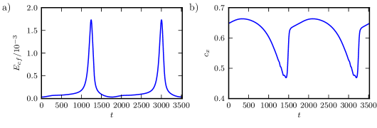
Figure 1: Energy and advection velocity of the edge state in ASBL at $Re=500$. The left frame shows the clear increase in energy when the edge state goes through the bursting phase. Studies of the flow field then show that afterwards it is displaced by half a box width, so that the full period are two bursting events in energy. The left frame shows the advection speed extracted by symmetry projection. It shows that as the energy goes up the structures slow down noticeably.

The full power of the method of comoving frames and the different dynamics in the laboratory and the comoving frame of reference is most prominently visible in the movie provided with the online material. To give some indication of the differences, we have extracted the spanwise velocity component at one point in the flow. The time trace in the labframe is shown in figure 2(a) and in the comoving frame of reference in figure 2(b). The high-frequency jitter on the signal in the labframe is due to the rapid advection in the downstream direction. In the comoving frame this is removed entirely, so that the gradual built up of a strong spanwise velocity and its rapid break down stands out clearly. The movie then shows that the velocity field during the low energy phase is dominated by down stream streaks with a weak sinusoidal modulation in the spanwise direction. As time goes on, the modulation amplitude increases, until the streaks break up. After the burst, the streaks and vortices form again, but displaced by half a box width in the spanwise direction.

The calculations are in a domain with periodic boundary conditions in the downstream and the spanwise directions. The flow naturally attains a discrete symmetry, a shift in the downstream direction by half a box length and a reflection on the midplane in the spanwise direction (Kreilos et al., 2013). With this discrete symmetry, the symmetry related advection velocities in the spanwise direction as calculated from (5) vanish exactly. For turbulent velocity fields this symmetry is broken and spanwise components do appear, as we discuss in §3.3.

Figure 2: Comparison of the edge state dynamics in the laboratory frame and the comoving frame of reference. Shown is the time evolution of a single spanwise velocity component, $w(0,1,L_{z}/4)$, as a function of time for one burst. In the laboratory frame of reference (left panel), the signal shows rapid oscillations, corresponding to the travelling-wave like behaviour of the edge state on short time scales, with the energetic burst visible as regions of larger amplitude oscillations. In the comoving frame of reference (right panel), the rapid oscillations are gone and the evolution of the component is rather smooth with an increase during the burst: the short-term dynamics has been completely eliminated and only the long-term dynamics are visible. A movie of the time evolution that shows the differences much more clearly is provided as supplementary material.

3.2 Spanwise advection of localized edge states

The discrete symmetry involving a spanwise reflection is broken if the domain is extended wide enough in the spanwise direction so that the state localizes. Edge states in this setting have been calculated in (Khapko et al., 2013b, a); their dynamics is similar to the one in periodic domains, and shows long calm phases that are interrupted by violent bursts, during which the structures break up and reform at a position that is shifted in the spanwise direction. These studies also show that different patterns in the spanwise displacement are possible: states may always be shifted to the right or the left, they may alternate between left and right shifts or they may even follow irregular patterns of left and right shifts. We here focus on a state that always shifts to the left.

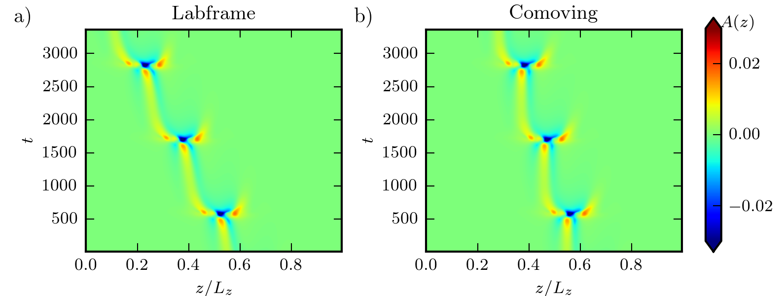
Figure 3: Space-time plot of the $x$-averaged wall-normal velocity $A(z,t)$, eq (8), for the left jumping edge state in a wide domain (Khapko et al., 2013b). The edge state is localized and during the calm phases between two bursts it consists of a pair of downstream-oriented counter-rotating vortices, visible by the alternating pattern of fluid moving up (red) and down (blue). At the bursts the structures break up and reform at a different spanwise location. a) In the laboratory frame, in the calm phases the red and blue lines are tilted, reflecting a spanwise drift. b) In the comoving frame of reference, the red and blue regions are aligned along the time-axis during the calm phases, indicating that the drift has been removed. However, the spanwise displacement at the bursts remains, indicating that it is not caused by advection but by internal dynamics of the flow.

In order to obtain a 2-d representation of the four-dimensional space-time evolution of the flow state we pick the wall-normal velocity at the height $\delta$ as a good indicator of up- and downwelling motion that can be connected to vortices. Since the domains are relatively short, we average this quantity in the downstream direction. The resulting observable

$$A(z,t)=\langle v(x,y=\delta,z,t)\rangle_{x}$$ (8)

depends on the spanwise coordinate $z$ and time $t$ and can be represented in 2-d color plots. For three periods of the left-shifting state we find the representation shown in figure 3. In the laboratory frame of reference (left panel), we see that there is an alternating pattern of fluid moving up and down (red and blue), corresponding to alternating streamwise vortices. At the bursts, the structures break up and are reformed almost symmetrically left and right, of which only the left one survives. In between the bursts the structures slowly and constantly drift to the left, as indicated by the finite slope of the lines. In the right panel, in the comoving frame of reference, the drift is completely removed and the structures are stationary in the calm phase, while they are still displaced at the bursts. This clearly shows that the method of comoving frames is able to separate the advective part of the time evolution (i.e. the drift) from the dynamically active and relevant part, in this case the break-up and displacement of the structures.

3.3 Spanwise drift of turbulent states

We now turn to turbulent flows and an analysis of spanwise shifts within the same computational domain as in §3.1. The general expression (5) for the phase speed with $\partial_{x}{\bf u}$ replaced by $\partial_{z}{\bf u}$ will not vanish in general (unless there are discrete symmetries as mentioned before). However, one would expect this contribution to be small and more or less uncorrelated. Indeed, the time traces in figure 4(a) show a strongly fluctuating signal with a small amplitude and a probability density function (pdf) that is well approximated by a Gaussian (figure 4(b)).

The correlation function of the advection speeds is shown in figure 5(a). It is based on data from 14 turbulent trajectories, each integrated for 200 000 time units. Initially, the correlation function falls of rather quickly, but then develops a wide background. As the inset shows, this background can be well approximated by an exponential form with a characteristic time of more than 4000 advective time units. Armed with the information that this correlation time is so long, one can begin to see evidence for it in figure 4(a), where the average of the fluctuations over the first 3000 time units is slightly above 0, whereas it is below zero for the remaining 7000 time units. The consequences of this are that the integrated advection speed, i.e. the distance over which the velocity field are displaced,

$$z_{0}(t)=\int_{0}^{t}c_{z}(\tau)d\tau,$$ (9)

first increases and then decreases. This is shown in figure 5(b).

Figure 4: Transverse advection velocity for a turbulent trajectory in the ASBL. a) The spanwise advection velocities $c_{z}$ are small and fluctuate randomly. b) The distribution of the advection velocities is almost perfectly Gaussian, indicating that it mainly consists of random noise.

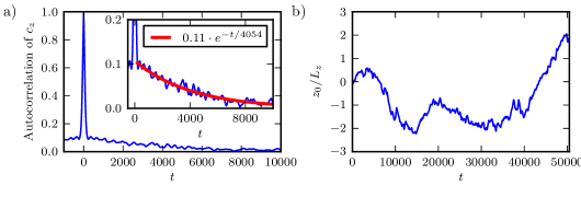
Figure 5: Correlation function and integrated displacements in spanwise direction in the ASBL. The correlation function of the spanwise advection speed (left frame) shows a strong central peak, indicative of weak correlations, and a broad background reaching out to very long times. The inset shows that this tail is well captured by an exponential distribution with a characteristic time of more than 4000 natural units. The frame on the right shows the integrated advection speed, or displacement, in the spanwise direction. The long correlations show up as modulations over very long periods. Note that the time scale covered is five times that shown in figure 4(a).

The effect of the transverse drift and its removal on the flow patterns is shown in figure 6, in the reduced representation (8) of the velocity fields. Regions with strongly positive or negative components in the normal direction show up as ridges that meander in space and time. This is particularly noticeable in the labframe (left frame). The black line on top of the figure is the integrated spanwise drift (9): it is perfectly aligned with the ridges in $A(z,t)$ and underlines the drift to the right. In the comoving frame of reference (right panel), the structures are then shifted by this amount in the spanwise direction, and the structures are more parallel to the vertical axis.

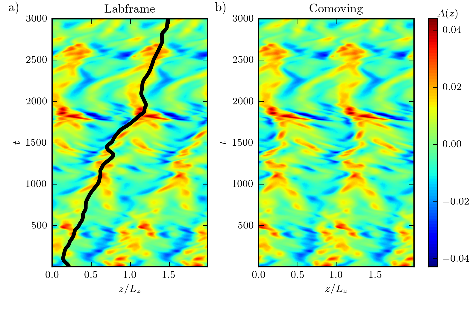
Figure 6: Space-time plot of the $x$-averaged wall-normal velocity $A(z,t)$, eq (8), demonstrating the effect of the method of comoving frames on a turbulent trajectory in the ASBL. The width of the box is twice the computation domain in order to highlight advection across the spanwise boundaries. For most times, there are two regions, predominantly blue and red, respectively, corresponding to one pair of large-scale downstream vortices. a) In the laboratory frame, the blue and red regions are tilted, reflecting a gradual spanwise drift. The thick black line is the integrated advection velocity, and it falls along a prominent ridge in the structures. b) In the comoving frame of reference, where the drift is subtracted, the two colored regions are essentially stationary and aligned along the time-axis.

In view of the long time correlations found in the spanwise direction, we also checked the downstream advection velocity. The downstream component fluctuates around a mean advection velocity $\overline{c}_{x}\approx 0.667$. The pdf is close to Gaussian with a weak but noticeable asymmetry to larger speeds, see igure 7(a). The autocorrelation function of the fluctuations around the mean, figure 7(b), falls off rapidly, but is significantly wider than the one for the spanwise shifts. The background is broader but less well characterized by a single exponential than in the case of the spanwise shift.

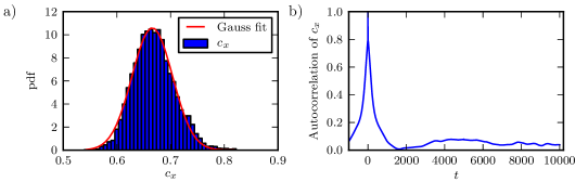
Figure 7: Pdf and autocorrelation function for the downstream advection velocity in the ASBL. In contrast to the spanwise advection, figure 5, it drops rather quickly to zero and does not show the long tails noted above.

4 Turbulent flow states in plane Poiseuille flow

In this section we apply the method of comoving frames to plane Poiseuille flow. As shown in (Toh & Itano, 2003; Zammert & Eckhardt, 2013), plane Poiseuille flow has exact coherent structures that are remarkably similar to the ones found in the ASBL, and their phase speeds in the streamwise and spanwise directions can be determined as in the case of the ASBL. We here focus on a turbulent state and its transverse drift.

We perform direct numerical simulations of plane Poiseuille flow with constant bulk velocity at $Re=3000$, based on the laminar center-line velocity $U_{0}$ and the channel half-width. The laminar flow profile is given by ${\bf u}(y)=(1-y^{2},0,0)$, so that the bulk velocity becomes $U_{bulk}=(2/3)U_{0}$. For the computations we use a domain of size $L_{x}\times L_{y}\times L_{z}=\pi\times 2\times 0.4\pi$, a resolution of $32\times 65\times 32$ modes, and Gibson’s code channelflow (Gibson, 2012).

As in §3.3 we study the spanwise and streamwise drifts. To calculate the correlation function of the advection speeds data from 20 turbulent trajectories, each integrated for 50 000 time units $d/U_{0}$ is used. The average of the downstream advection velocity $c_{x}$ is $0.675$ and therefore slightly larger than the bulk velocity. As in the ASBL, the probability density function of $c_{x}$ in figure 8(a) is well approximated by a Gaussian and the correlation function of the downstream advection velocities, shown in figure 8(b), quickly drops to zero.

The spanwise advection velocities are also Gaussian distributed with a mean value of zero (not shown). The correlation function for the spanwise velocities in figure 8(c) also shows a wide background as in the case of the ASBL. An exponential fit yields a characteristic time of about 300 time units. This weak long-ranged correlation can be seen in the integrated advection speeds $z_{0}$ (9) in figure 8(d). The plot reveals several segments in which the flow drifts in the same direction. They are a few hundred time units long, consistent with the correlation time of about 300.

The different transverse correlation times are unusual. Compared to the ASBL the characteristic times of the background correlation differ by a factor of 13. Yet the coherent structures studied by Toh & Itano (2003) and Zammert & Eckhardt (2013) show bursts on time scales that are similar. The difference presumably comes about because the coherent structures in plane Poiseuille flow are localized near one wall, whereas the determination of the advection speed involves an integration over the entire domain. Uncorrelated motions close to the upper and lower walls will thus reduce the correlation time.

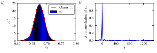
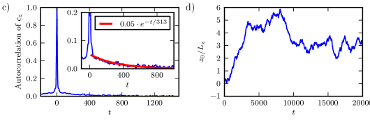
Figure 8: Application of the method of comoving frames to plane Poiseuille flow at $Re=3000$. (a) The streamwise advection velocity fluctuates around a mean value of $0.675$ what is close to the bulk velocity. The distribution of the velocities is almost gaussian. (b) The correlation function of the downstream advection velocity quickly drops to zero. (c) The correlation function of the spanwise advection speed shows a strong central peak, indicative of weak correlations, and a broad background reaching out to long times. The inset shows that this tail is well captured by an exponential distribution with a characteristic time of about 300 time units. In (d) the the integrated advection speed, or displacement, in the spanwise direction is shown.

5 Concluding remarks

The examples show that one of the appealing features of the transformation (5) is the local and instantaneous removal of a downstream advective component in the time evolution. The speed by which this component is removed depends on the state and hence varies in time. However, once this component is removed, the changes in vortices and streaks stand out much more clearly and become accessible to further analysis.

It is possible to extend this analysis from local in time also to local in space, and to find advection speeds that focus on particular features of the flow. The key to this is the scalar product that enters the projection to obtain eq. (5). In the calculations shown here we use the usual Euclidian scalar product with the scalar product of all components integrated over all of space, eq. (2.6). For other situations and applications, suitable adaptations of the method are possible. For instance, if not all velocity components are available, one could base the projection on a subset of components. Also, if the velocity fields are only known in a subset of the space, the integration may be limited to that subset. Extensions in this direction are currently being explored.

Another extension of the method uses different representations of the velocity field, e.g. expansions in spectral modes and restrictions in the scalar product to subsets of the modes. For instance, if the velocity fields are given in a Fourier representation, one can extract phase speeds for individual Fourier components. Del Álamo & Jiménez (2009) used such an idea in their intriguing discussion of the effects of Taylors frozen flow hypothesis (Taylor, 1938; Townsend, 1980; Zaman & Hussain, 1981) on turbulent spectra: they defined a wavenumber dependent phase speed (their equation (2.4)) that is equivalent to (5) when applied to a single spanwise Fourier mode.

The method for the extraction of symmetry related motions and the expression for the advection speed given in equation (5) are easy to calculate and to extract from both numerical and experimental data. For the use with experimental data, the time-evolution vector is replaced by finite differences between velocity fields at different times, and the spatial derivative can be approximated by finite differences in space. With a sufficiently good spatial and temporal resolution, the results are indistinguishable from full analytical approximations. If the time steps are longer it may be advisable to turn to the optimization methods described in Mellibovsky & Eckhardt (2012), where the velocity field ${\bf u}(x,y,z,t)$ is used as a template and a suitable shift is determined by minimizing $||({\bf u}(x,y,z,t+\Delta T)-{\bf u}(x-\Delta x,y,z,t)||^{2}$. The shift and advection speed determined by this method and the one from eq. (5) become equivalent in the limit of small $\Delta t$ where Taylor expansions are possible.

Continuous symmetries appear in many fields, and various methods for separating shifts along the symmetry axis from dynamical changes have been developed (see Cvitanović et al. (2012a); Froehlich & Cvitanović (2012); Cvitanović et al. (2012b)). In the fluid mechanical context they have appeared in connection with derivations of low-dimensional models using proper orthogonal decomposition (Rowley & Marsden, 2000; Rowley et al., 2003). Their relevance for the detection of relative periodic orbits, including a successul application of the method of slices, which allows an exact symmetry reduction, has been emphasized in Willis et al. (2013).

The method of comoving frames described in §2 helps in removing some of the advective and dynamically less relevant components, but it does not solve all problems related to finding relative periodic orbits, since it is not a general symmetry reduction scheme. For instance, the state shown in the first example in §3 passes through an intermediate state where the flow fields are shifted by half a box width in the spanwise direction. This shift is a dynamic one, not related to advection, and hence not removed. Therefore, for a periodic orbit calculation, one would still have to take the initial state and its images under discrete symmetries and check whether the flow returns to the symmetry related copy. The situation gets even more complicated for the states in the wider domains as discussed in Khapko et al. (2013b, a): For instance, the states that steadily move to the left do repeat after a suitable shift in the spanwise direction, but as shown in §3.2 this translation is again not removed by the continuous shifts since it is a result of the changes in the flow fields.

Nevertheless, judging by the examples we have analyzed so far, the removal in particular of the downstream advection reveals underlying coherent structures, or candidates for coherent structures, more clearly than the laboratory frame dynamics.

Acknowledgements

We thank John F Gibson for providing and maintaining the open source Channelflow.org code, Marc Avila for discussions that motivated this investigation, Predrag Cvitanović for extensive exchanges on continuous symmetries, Hannes Brauckmann and Matthew Salewski for comments and Francesco Fedele for encouragement. This work has been supported in part by the Deutsche Forschungsgemeinschaft within Forschergruppe FOR1182.

References

- Clever & Busse (1997) Clever, R M & Busse, F H 1997 Tertiary and quaternary solutions for plane Couette flow. J. Fluid Mech. 344, 137–153.
- Cvitanović et al. (2012a) Cvitanović, P, Artuso, R, Mainieri, G, Tanner, G & Vattay, G 2012a Chaos: Classical and quantum, 14th edn. ChaosBook.org Niels Bohr Institute Copenhagen.
- Cvitanović et al. (2012b) Cvitanović, P, Borrero-Echeverry, D, Carroll, K M, Robbins, B & Siminos, E 2012b Cartography of high-dimensional flows: a visual guide to sections and slices. Chaos 22, 047506.
- Del Álamo & Jiménez (2009) Del Álamo, J C & Jiménez, J 2009 Estimation of turbulent convection velocities and corrections to Taylor’s approximation. J. Fluid Mech. 640, 5–26.
- Fransson & Alfredsson (2003) Fransson, J H M & Alfredsson, P H 2003 On the disturbance growth in an asymptotic suction boundary layer. J. Fluid Mech. 482, 51–90.
- Froehlich & Cvitanović (2012) Froehlich, S & Cvitanović, P 2012 Reduction of continuous symmetries of chaotic flows by the method of slices. Commun. Nonlinear Sci. Numer. Simul. 17 (5), 2074–2084.
- Gibson (2012) Gibson, J F 2012 Channelflow: A spectral Navier-Stokes simulator in C++. Tech. Rep.. U. New Hampshire.
- Gibson et al. (2008) Gibson, J F, Halcrow, J & Cvitanović, P 2008 Visualizing the geometry of state space in plane Couette flow. J. Fluid Mech. 611, 107–130.
- Gibson et al. (2009) Gibson, J F, Halcrow, J & Cvitanović, P 2009 Equilibrium and traveling-wave solutions of plane Couette flow. J. Fluid Mech. 638, 243–266.
- Khapko et al. (2013a) Khapko, T, Duguet, Y, Kreilos, T, Schlatter, P, Eckhardt, B & Henningson, D S 2013a Complexity of localised coherent structures in a boundary-layer flow. arXiv:1308.5531 .
- Khapko et al. (2013b) Khapko, T, Kreilos, T, Schlatter, P, Duguet, Y, Eckhardt, B & Henningson, D S 2013b Localized edge states in the asymptotic suction boundary layer. J. Fluid Mech. 717, R6.
- Kreilos et al. (2013) Kreilos, T, Veble, G, Schneider, T M & Eckhardt, B 2013 Edge states for the turbulence transition in the asymptotic suction boundary layer. J. Fluid Mech. 726, 100–122.
- Mellibovsky & Eckhardt (2012) Mellibovsky, F & Eckhardt, B 2012 From travelling waves to mild chaos: a supercritical bifurcation cascade in pipe flow. J. Fluid Mech. 709, 149–190.
- Nagata (1990) Nagata, M 1990 Three-dimensional finite-amplitude solutions in plane Couette flow: bifurcation from infinity. J. Fluid Mech. 217, 519–527.
- Nagata (1997) Nagata, M 1997 Three-dimensional traveling-wave solutions in plane Couette flow. Phys. Rev. E 55, 2023–2025.
- Rowley et al. (2003) Rowley, C W, Kevrekidis, I G, Marsden, J E & Lust, K 2003 Reduction and reconstruction for self-similar dynamical systems. Nonlinearity 16, 1257–1275.
- Rowley & Marsden (2000) Rowley, C W & Marsden, J E 2000 Reconstruction equations and the Karhunen–Loève expansion for systems with symmetry. Phys. D Nonlinear Phenom. 142 (1-2), 1–19.
- Schlichting (1982) Schlichting, H 1982 Grenzschicht Theorie, 8th edn. Verlag G. Braun.
- Schneider et al. (2008) Schneider, T M, Gibson, J F, Lagha, M, De Lillo, F & Eckhardt, B 2008 Laminar-turbulent boundary in plane Couette flow. Phys. Rev. E 78, 37301.
- Smale (1970) Smale, S. 1970 Topology and mechanics. I. Invent. Math. 10 (4), 305–331.
- Taylor (1938) Taylor, G I 1938 The Spectrum of Turbulence. Proc. R. Soc. A Math. Phys. Eng. Sci. 164 (919), 476–490.
- Toh & Itano (2003) Toh, S & Itano, T 2003 A periodic-like solution in channel flow. J. Fluid Mech. 481, 67–76.
- Townsend (1980) Townsend, A A 1980 The structure of turbulent shear flow. Cambridge University Press.
- Viswanath (2007) Viswanath, D 2007 Recurrent motions within plane Couette turbulence. J. Fluid Mech. 580, 339–358.
- Waleffe (2003) Waleffe, F 2003 Homotopy of exact coherent structures in plane shear flows. Phys. Fluids 15, 1517–1534.
- Wang et al. (2007) Wang, J, Gibson, J F & Waleffe, F 2007 Lower branch coherent states in shear flows: Transition and control. Phys. Rev. Lett. 98, 6–8.
- Willis et al. (2013) Willis, A P, Cvitanović, P & Avila, M 2013 Revealing the state space of turbulent pipe flow by symmetry reduction. J. Fluid Mech. 721, 514–540.
- Zaman & Hussain (1981) Zaman, K. B. M. Q. & Hussain, a. K. M. F. 1981 Taylor hypothesis and large-scale coherent structures. J. Fluid Mech. 112, 379.
- Zammert & Eckhardt (2013) Zammert, S & Eckhardt, B 2013 Periodically bursting edge states in plane Poiseuille flow. arXiv:1312.6783 .