Effects of Nonlinear Coupling on Spatiotemporal Regularity

Abstract

In this work we investigate the spatiotemporal behaviour of lattices of coupled chaotic logistic maps, where the coupling between sites has a nonlinear form. We show that the stable range of the spatiotemporal fixed point state is significantly enhanced for increasingly nonlinear coupling. We demonstrate this through numerical simulations and linear stability analysis of the synchronized fixed point. Lastly, we show that these results also hold in coupled map lattices where the nodal dynamics is given by the Gauss Map, Sine Circle Map and the Tent Map.

Keywords: Synchronization; Coupled maps; Nonlinear coupling; Spatiotemporal Regularity.

1 Introduction

Coupled Map Lattices (CML) is a class of models that have been used to describe many spatially extended complex systems [1, 2], ranging from ecological networks [3, 4, 5] to nematic liquid crystals [6]. The basic ingredients of a CML model is the local dynamics at the sites of the lattice and the coupling interaction between subsets of the sites. In recent years researchers have extensively explored the effect of different coupling topologies on the dynamics of coupled dynamical systems and found remarkable phenomenon such as spatiotemporal synchronization. Network topology has been considered the key to obtaining a stable synchronization manifold in coupled chaotic systems [7, 8]. However the effect of the form of the coupling function on spatiotemporal patterns has not gained much research attention. In this work we address this issue and show that the nonlinear coupling forms have a pronounced effect on spatio-temporal synchronization in coupled map systems. Our central results is that nonlinear coupling stabilizes the synchronization manifold, even for regular networks where average path length is too high to sustain a stable synchronization manifold.

Model: We consider $N$ chaotic maps on an ring. The sites are denoted by the index $i=1,2\dots N$, where $N$ is the system size. Each node is coupled to its two nearest neighbors i.e. the $i^{th}$ site is connected to site $(i+1)^{th}$ and $(i-1)^{th}$ node. The general time evolution equation of $i^{th}$ node is given by

$$x^{i}_{n+1}=(1-\epsilon)f(x^{i}_{n})+\frac{\epsilon}{2K}\sum_{j=1}^{K}(g(x^{i-j}_{n})+g(x^{i+j}_{n}))$$ (1)

In this work we will consider $K=1$, namely each site couples to two nearest neighbours. In the language of networks $i$ represents a node of degree $2$ in the network. The function $f(x)$ gives the local dynamics. To begin with, this is chosen to be the prototypical chaotic map, the logistic map: $x_{n+1}=rx_{n}(1-x_{n})$, where the nonlinearity parameter $r$ is chosen to be $4$. The strength of coupling is denoted by $\epsilon$, and the function $g(x)$ is the coupling function. The $(1-\epsilon)$ term weighting the local map $f(x)$ keeps the system bounded by confining the dynamics of the nodes in the interval $[0:1]$.

The central focus of this work is to explore the behaviour of this system under coupling of the form:

$$g(x)=x^{q}$$ (2)

where $q=1,2,3,\dots\infty$. Since $x\leq 1$, in this class of examples, increasing power of $x$ yield smaller magnitude of the coupling term.

In the sections below we will present our results from extensive numerical simulations and stability analysis, describing the effects of varying $q$ in the coupling function, on spatiotemporal patterns. Notably, we will show that increasingly nonlinear coupling forms yield larger stable ranges for the spatiotemporal fixed point.

Numerical Results

First we will demonstrate numerically that nonlinear coupling forms enhance spatiotemporal regularity in coupled maps. The numerical results here have been obtained for large set of random initial conditions $(500-1000)$, with network size $N$ ranging from $10$ to $1000$. Figure-1a displays the bifurcation diagram for the linear coupling with strictly nearest neighbors case.

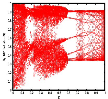
(a) Linear coupling

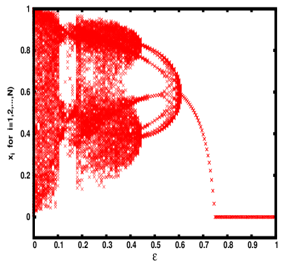
(b) Quadratic coupling

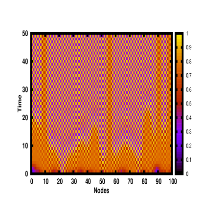
(c) Linear coupling

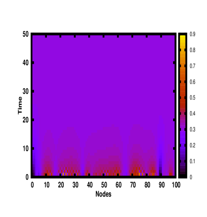
(d) Quadratic coupling

Figure 1: Subfigure (a) and (b): Bifurcation diagram showing values of $x_{n}^{i}$ with respect to coupling strength $\epsilon$, for coupled logistic maps with linear coupling ($q=1$ in Eqn. 1-2) and quadratic coupling ($q=2$ in Eqn. 1-2). Here the size of the lattice is $N=100$. In the figure we plot $x_{n}^{i}(i=1,...,100)$ over $n=1,...,10$ iterations (after a transience time of $5000$) for ten different initial conditions.
Subfigure (c) and (d): Showing spatio-temporal dynamics of system for coupling strength $\epsilon=0.72$ for coupled logistic maps with linear coupling and quadratic coupling.

It is evident here that linear coupling scheme with strictly regular connections does not show any stable spatiotemporal manifold in system. To quantify the synchronization we define the range of synchronization as $R=(1-\epsilon_{sync})$. Here $\epsilon_{sync}$ is the value of $\epsilon$ where synchronization manifold starts getting stabilized. In case of linear coupling $R$ is zero.

We start with the effect of the quadratic coupling form ($g(x)=x^{2}$) on the dynamics of coupled maps. Figure-1b displays the bifurcation diagram for quadratic coupling, clearly showing the enhancement of the spatiotemporal fixed point regime in system. Notice that the invariant synchronization manifold is an $\epsilon$ dependent curve.

We then go on to study the system with coupling function $g(x)=x^{q}$ with increasing $q$. Our central observation is that the range of the spatiotemporal fixed point, $R$, is dependent on $q$. As we increase the nonlinearity in coupling we get a larger range of synchronization (figure-2, 3). Also, The stable range of the spatiotemporal fixed point soon converges to a maximum $R_{max}$ as we increases $q$ further. It is worth noting that when we take large value of $q$, the individual nodes follow the dynamics of synchronized logistic map, with an inverted bifurcation sequence arising from a rescaled nonlinearity parameter (figure:5).

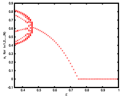
(a) $x^{3}$ coupling

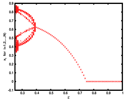
(b) $x^{4}$ coupling

Figure 2: Bifurcation diagram showing values of $x_{n}^{i}$ with respect to coupling strength $\epsilon$, for coupled logistic maps with coupling form $g(x)=x^{3}$ and $g(x)=x^{4}$. This figure shows how range of spatiotemporal fixed points increases as we increase the nonlinearity in coupling form. Here the size of the lattice is $N=100$. In the figure we plot $x_{n}^{i}(i=1,...,100)$ over $n=1,...,10$ iterations (after a transience time of $5000$) for ten different initial conditions.

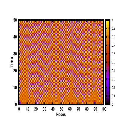
(a) Linear coupling

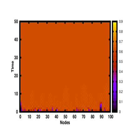
(b) Quartic coupling

Figure 3: Spatio-temporal dynamics of system for coupling strength $\epsilon=0.42$ for coupled logistic maps with linear coupling and Quartic ($x^{4}$) coupling.

We find the range of the spatiotemporal fixed point, numerically, for different $q$. The results are displayed in Figure-4. Further, we obtain the functional dependence of the coupling strength at which the spatiotemporal fixed point gains stability, denoted by $\epsilon_{sync}$, on $q$. It is clear that $\epsilon_{sync}$ converges to a minimum value with increasing $q$, namely $\lim\limits_{q\to\infty}\epsilon_{sync}=\epsilon_{min}$.

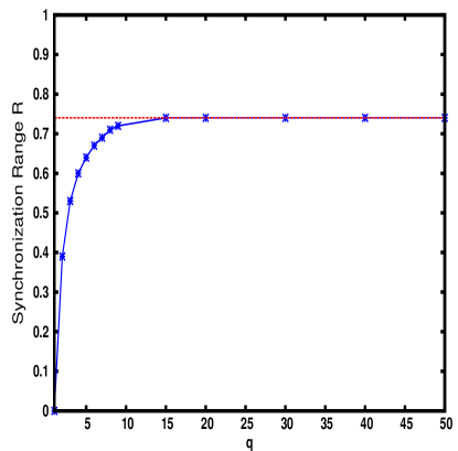
(a) Synchronization Range

(b) Least square fitting

Figure 4: Characterizing the dependence of Range on $q$. (a) Numerically calculated ranges R for many q’s. (b) Best fitting for $\epsilon_{sync}$ vs $q$

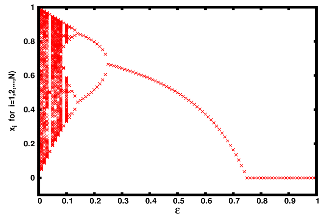
Figure 5: Inverted Logistic map: Bifurcation diagram showing values of $x_{n}^{i}$ with respect to coupling strength $\epsilon$, for coupled logistic maps with $x^{100}$ coupling ($q=100$ in Eqn. 1-2).

In order to understand the coupling strength necessary to stabilize the spatiotemporal fixed point, we attempted to fit the values of $\epsilon_{sync}$ obtained for increasing values of $q$, to different functional forms. We found reasonably good fit to the form:

$$\epsilon_{sync}=\frac{a}{q^{b}}+c$$ (3)

with parameters values $a=0.977\pm 0.063$, $b=1.1415\pm 0.078$ and $c=0.251\pm 0.004$.

In the next section we will analyse the system to gain more understanding of the effect of nonlinear coupling forms on spatiotemporal regularity.

Analysis

Mathematically, the synchronization manifold is the state of system when all nodes follow same trajectory i.e. $x^{1}=x^{2}=\dots=x^{N}$, and for the temporal fixed point we must have: $x^{i}_{n+1}=x^{i}_{n}=x^{*}$ for $i=1,\dots,N$, where $x^{*}$ is the spatiotemporal fixed point. Combinedly, these two equations result following one equation which can be solved to compute spatiotemporal fixed point.

$$x^{*} =(1-\epsilon)rx^{*}(1-x^{*})+\frac{\epsilon}{2}\sum_{j=1}^{2}(x^{*})^{q}$$ (4)

$$\epsilon x^{q} -(1-\epsilon)rx^{2}+(r-r\epsilon-1)x=0$$ (5)

For linear coupling, i.e. $q=1$, and for $r=4$, solution of above equation-5 are

$$x=0\quad or\quad x =0.75$$

So linear coupling gives two $\epsilon$ independent fixed points.

In case of quadratic coupling ($q=2$), equation-5 provides following two solutions:

$$x=0\quad or\quad x =\frac{-3+4\epsilon}{-4+5\epsilon}$$

In this case, one of the solutions is coupling strength, $\epsilon$, dependent. We compare this solution with numerical simulations (figure-1b) and get exact match as it is clearly shown in figure-6.

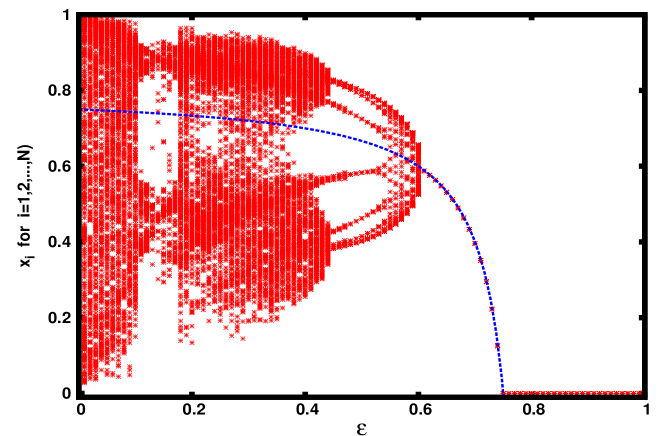
Figure 6: Spatiotemporal fixed points for the case of quadratic coupling. Here the points marked with crosses are obtained numerically, and the dashed line is the analytical solution.

By following the same approach as above, we can analytically find the spatiotemporal fixed points for any $q$.

Note that the limit of $q$ tending to infinity is interesting because we have $0\leq x_{n}\leq 1$ for all $n$, that implies $\lim\limits_{q\to\infty}(x_{n})^{q}\backsimeq 0$. So evolution equations of system can be written as

$$x^{i}_{n+1}=(1-\epsilon)rx^{i}_{n}(1-x^{i}_{n})+0$$

This equation is nothing but the inverted logistic map with effective nonlinearity parameter $r(1-\epsilon)$. Bifurcation diagram is shown in figure:5.

Linear stability analysis of the spatiotemporal fixed points

In the previous section we calculated the fixed points for the nonlinear coupling case. Now we will check the stability of these fixed points using standard linear stability analysis [9] .

Linear coupling : As calculated above, there exists two spatiotemporal fixed points in the linear coupling case, and simulations showed that both are unstable. So we expect that the maximum magnitude of eigenvalues of Jacobian matrix, calculated around these two fixed points, should be greater than $1$. In order to check this, we analytically find the eigenvalue spectrum of the Jacobian matrix [10] and plot the magnitude of largest eigenvalue, with respect to coupling strength $\epsilon$. The results are displayed in Figure 7.

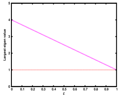
(a) Fixed Point at Zero

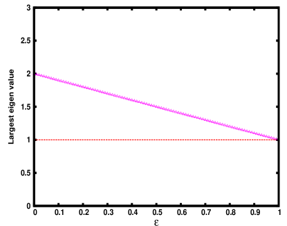
(b) Nonzero Fixed Point

Figure 7: Magnitude of largest eigenvalue vs $\epsilon$ plot for linear coupling.

Figure-7 exactly matches the numerical results, and shows that there is no stable spatio-temporal fixed point state as the magnitude of largest eigenvalue is always greater than $1$ for both fixed points.

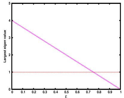
(a) Fixed Point at Zero

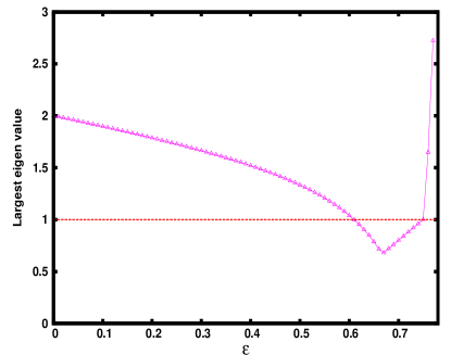
(b) Nonzero Fixed Point

Figure 8: Magnitude of largest eigenvalue vs $\epsilon$ plot for quadratic coupling.

For the quadratic coupling case ($q=2$) results are displayed in the Figure 8. It is evident here that the fixed point at zero is stable for $0.75\leq\epsilon\leq 1$ because the maximum magnitude of eigenvalues is smaller than $1$ for this $\epsilon$ range. On the other hand the non-zero fixed point is stable for $0.61\leq\epsilon\leq 0.75$. These ranges are exactly as observed in the numerical simulations (cf. bifurcation diagram in Figure 1b).

So it is clear from the analysis above that we can analytically predict the stability of the spatiotemporal fixed points, qualitatively as well as quantitatively.

Generality of the Results

In order to examine the range of applicability of the phenomena observed above, we will implement the same coupling scheme in coupled map lattices with different local dynamics. In particular we will demonstrate below how nonlinear coupling yields enhanced stable regimes for the spatiotemporal fixed point state, in a system whose local evolution is given by the Gauss Map, Sine-Circle map and by the Tent Map.

The Gauss Map is given as follows:

$$x_{n+1}=e^{-\alpha x_{n}^{2}}+\beta$$

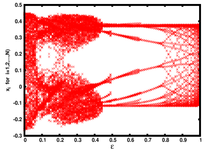
(a) Linear coupling

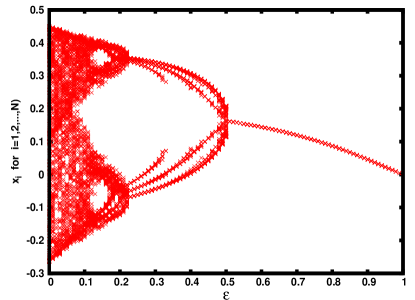
(b) Quadratic Coupling

Figure 9: Bifurcation diagram showing values of $x_{n}^{i}$ with respect to coupling strength $\epsilon$, for coupled Gauss maps with linear coupling ($q=1$ in Eqn. 1-2) and quadratic coupling ($q=2$ in Eqn. 1-2). Here the size of the lattice is $N=100$. In the figure we plot $x_{n}^{i}(i=1,...,100)$ over $n=1,...,10$ iterations (after a transience time of $5000$) for ten different initial conditions.

It shows chaotic dynamics for parameter values $(\alpha,\beta)=(-6.2,0.55)$. Now we take this chaotic map as our local dynamics and simulate the dynamics of system for quadratic ($g(x)=x^{2}$) as well as linear coupling. The results are presented in Figure 10. It is clear from the figure that we get a stable range for the spatiotemporal fixed point state when the coupling is nonlinear, while linear coupling does not give any stable range.

The Tent Map is given as follows:

$$x_{n+1}=\begin{cases}rx,&x\leq\frac{1}{2}\\ r(1-x),&\frac{1}{2}\leq x\leq 1\\ \end{cases}$$

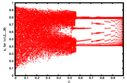
(a) Linear coupling

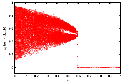
(b) Quadratic Coupling

Figure 10: Bifurcation diagram showing values of $x_{n}^{i}$ with respect to coupling strength $\epsilon$, for coupled Tent maps with linear coupling ($q=1$ in Eqn. 1-2) and quadratic coupling ($q=2$ in Eqn. 1-2). Here the size of the lattice is $N=100$. In the figure we plot $x_{n}^{i}(i=1,...,100)$ over $n=1,...,10$ iterations (after a transience time of $5000$) for ten different initial conditions.

(a) Linear coupling

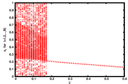
(b) Quadratic Coupling

Figure 11: Bifurcation diagram showing values of $x_{n}^{i}$ with respect to coupling strength $\epsilon$, for coupled Sine circle maps with linear coupling ($q=1$ in Eqn. 1-2) and quadratic coupling ($q=2$ in Eqn. 1-2). Here the size of the lattice is $N=100$. In the figure we plot $x_{n}^{i}(i=1,...,100)$ over $n=1,...,10$ iterations (after a transience time of $5000$) for ten different initial conditions.

We choose the chaotic Tent Map with parameter value $r=1.9$ as the local dynamics. Results displayed in Figure 10 clearly depict that while linear-coupled lattices of chaotic Tent maps do not yield any stable spatiotemporal fixed point regimes, the spatio-temporal fixed point state gains stability under nonlinear coupling.

Lastly, we take Sine circle map as local dynamics which has following equation:

$$x_{n+1}=x_{n}+\omega-\frac{K}{2\pi}sin(2\pi x_{n})\quad\quad(mod)1$$

For parameter values $\omega=0.5$ and $K=3$ it is a chaotic function. Results presented in figure-11 clearly show the enhanced regularities in dynamics when we take nonlinear coupling.

Conclusions

In conclusion we have investigated the spatiotemporal behaviour of lattices of coupled chaotic logistic maps, where the coupling between sites has a nonlinear form. We showed that the stable range of the spatiotemporal fixed point state is significantly enhanced for increasingly nonlinear coupling. We demonstrated this through numerical simulations and linear stability analysis of the synchronized fixed point. Also, we showed that these results also hold in coupled map lattices where the nodal dynamics is given by the Gauss Map, Sine Circle Map and the Tent Map.

The results here can be put in a following broader perspective: it is of considerable interest to find out what form of coupling and connection topologies allows the spatiotemporal fixed point of a collection of strongly chaotic elements to gain stability. This is of interest in the context of control, in both human engineered systems and in extended complex systems arising in the natural world [7, 11]. For instance, earlier studies had shown that dynamical random rewiring of links, namely changing the form of the connectivity matrix, stabilized the spatiotemporal fixed point in networks of chaotic elements [8]. Here we show an alternate route to achieving spatiotemporal regularity, by demonstrating how in a regular lattice of chaotic maps we can achieve a stable synchronized fixed point by nonlinear coupling forms.

Acknowledgement

I am deeply thankful to my masters project guide Prof. Sudeshna Sinha for her guidance, help and encouragement. Also I thank to Mr. Anshul Choudhary and Anshu Gupta for their fruitful discussions. I dedicate this work to my family.

References

- [1] K. Kaneko. Theory and Applications of Coupled Map Lattices (Nonlinear Science: Theory and Applications). Wiley, 1 edition, 3 1993.
- [2] Arkady Pikovsky, Michael Rosenblum, and Jürgen Kurths. Synchronization: A Universal Concept in Nonlinear Sciences (Cambridge Nonlinear Science Series). Cambridge University Press, 1 edition, 5 2003.
- [3] G. Cocho and G. Martínez-Mekler. On a coupled map lattice formulation of the evolution of genetic sequences. Phys. D, 51(1-3):119–130, September 1991.
- [4] Michael Bevers and Curtis H. Flather. Numerically exploring habitat fragmentation effects on populations using cell-based coupled map lattices. Theoretical Population Biology, 55, 1999.
- [5] McGlade J.M. Hendry, R.J. and J. Weiner. A coupled map lattice model of the growth of plant monocultures. Ecological Modelling, 84, 1996.
- [6] S. M. Kamil, Sudeshna Sinha, and Gautam I. Menon. Regular and chaotic states in a local map description of sheared nematic liquid crystals. Phys. Rev. E, 78:011706, Jul 2008.
- [7] Prashant M Gade and Chin-Kun Hu. Scaling and universality in transition to synchronous chaos with local-global interactions. Phys Rev E Stat Nonlin Soft Matter Phys, 73:036212, 2006.
- [8] Sudeshna Sinha. Random coupling of chaotic maps leads to spatiotemporal synchronization. Phys. Rev. E, 66:016209, Jul 2002.
- [9] Louis M. Pecora and Thomas L. Carroll. Master stability functions for synchronized coupled systems. Phys. Rev. Lett., 80:2109–2112, Mar 1998.
- [10] Steven H. Strogatz. Nonlinear Dynamics And Chaos: With Applications To Physics, Biology, Chemistry, And Engineering (Studies in Nonlinearity). Westview Press, 1 edition, 1 2001.
- [11] Louis M. Pecora and Thomas L. Carroll. Synchronization in chaotic systems. Phys. Rev. Lett., 64:821–824, Feb 1990.