Influence of vibrations on electron transport through nanoscale contacts

Abstract

In this article we present a novel semi-analytical approach to calculate first-order electron-vibration coupling constants within the framework of density functional theory. It combines analytical expressions for the first-order derivative of the Kohn-Sham operator with respect to nuclear displacements with coupled-perturbed Kohn-Sham theory to determine the derivative of the electronic density matrix. This allows us to efficiently compute accurate electron-vibration coupling constants.We apply our approach to describe inelastic electron tunneling spectra of metallic and molecular junctions. A gold junction bridged by an atomic chain is used to validate the developed method, reproducing established experimental and theoretical results. For octanedithiol and octanediamine single-molecule junctions we discuss the influence of the anchoring group and mechanical stretching on the inelastic electron tunneling spectra.

1 Introduction

The advances in nanoscience over the past couple of decades have made it possible to probe charge transport in nanoscale systems down to the single-molecule and single-atom level [1, 2, 3]. With such measurements becoming increasingly routine, less explored effects such as self-heating in nanojunctions due to current flow move into the focus of research [4, 5, 6, 7]. In this context, electron-vibration (EV) interactions play a crucial role in dissipating the heat of electrons by transferring it to the vibrational degrees of freedom. Beside this, inelastic processes can lead to discernible signatures in transport quantities that can be exploited to characterize nanoscale conductors. This latter aspect is the subject of the present paper.

The EV interaction can significantly influence transport properties. Thus it may lead to phonon drag [8, 9, 10], thermally activated transport in long molecular wires [11], current saturation at a high applied voltage bias [12, 13], or electromigration as well as junction breakdown due to current-induced forces and local heating [14, 15, 16, 17, 18]. Inelastic EV scattering is also used to characterize molecular and atomic junctions spectroscopically. Depending on the conductance regime, the techniques are either called inelastic electron tunneling (IET) spectroscopy [19, 20, 21] or point contact spectroscopy [1, 22]. In both cases, however, the second derivative $\mbox{d}^{2}I/\mbox{d}V^{2}$ of the electrical current $I$ with respect to the applied bias voltage $V$ is measured. For simplicity we will refer to both techniques as IET spectroscopy in the following.

In the IET spectroscopy, which is the central subject of this study, the excitation of a vibrational mode inside the junction gives rise to a characteristic signature in the current-voltage characteristics. Especially for molecular junctions, it has become an important tool to identify the molecule that bridges two metal electrodes and to determine the precise contact geometry [23, 24, 25, 26, 27, 28]. For the theoretical description of the EV interaction in nanoscale conductors, various different approaches exist, which can deal with the whole regime from weak to intermediate to strong EV couplings [4, 29, 30, 31, 32]. While model calculations are able to capture experimentally observed effects on a qualitative level, a fully atomistic theory is necessary for their material-dependent, quantitative interpretation. Density functional theory (DFT) provides such an atomistic electronic structure description for molecular, solid-state, and hybrid systems. Despite the fact that DFT is not a quasi-particle method, it is often used to calculate transport properties of nanoscale junctions in combination with non-equilibrium Green’s function (NEGF) techniques. Approximate DFT tends to underestimate the band gap of bulk semiconductors or insulators as well as the gap between the highest occupied and lowest unoccupied molecular orbital of molecular systems. Typically, this leads to an overestimation of the conductance of molecular junctions. To compensate for these shortcomings, a “self-energy corrected” DFT scheme has been developed to obtain more accurate quasiparticle energies [33] or even time-consuming atomistic quasiparticle methods were employed within the GW approximation [34]. For metallic systems, including metallic atomic contacts, where the “band gap problem” of DFT does not arise, the quantum transport calculations using the combination of DFT and NEGF (DFT+NEGF) show often good agreement with experiment [35].

Quantities derived from the total ground-state energy like bond lengths, binding energies and vibrational spectra are commonly described reliably for molecular and solid-state systems within the DFT schemes using the local density approximation (LDA) or generalized gradient approximation (GGA) [36, 37, 38]. Due to the reasonable compromise between computational cost and accuracy, DFT+NEGF has become the standard method for the atomistic, first-principles modeling of transport through nanoscale devices. The DFT+NEGF approach is very compelling, when inelastic corrections to the current due to the EV interaction are of interest, since it allows for the consistent treatment of the whole system [35]: The electronic structure, the vibrational modes, as well as their coupling can all be described within the same method. In DFT+NEGF the EV coupling is usually treated in the weak limit either by means of a lowest-order expansion (LOE) or the self-consistent Born approximation [35, 39, 40, 41].

In this work we extend our cluster-based approach for determining elastic quantum transport to include the inelastic corrections at the level of the LOE in the EV coupling. For a detailed discussion of the LOE and of the cluster-based transport approach, we refer to our previous works in Refs. [40, 42]. We do not pursue the direction of “self-energy corrected” DFT or atomistic quasiparticle electronic structure methods here, but use the benefit of DFT to describe the coupled system of electrons and phonons in atomic and molecular junctions within a single, unified atomistic approach. We focus particularly on the calculation of the EV coupling constants within the framework of DFT. We have implemented a scheme that computes the EV couplings, similar to the phonon modes, using density functional perturbation theory (DFPT). The use of a Gaussian basis allows us to calculate the required matrix elements semi-analytically. In this way, we avoid finite differences, increase the computational efficiency, and prevent numerical instabilities especially for the low-frequency modes [43]. We test the newly developed method at monovalent gold (Au) atomic junctions and reproduce literature results for a well-studied atomic chain configuration. Finally, we discuss the inelastic signals in molecular junctions. Elaborating on theoretical aspects of our previous work in Ref. [28], we study the IET spectra of octane-based single-molecule junctions with thiol and amine anchors. We focus especially on vibrations localized on the octane molecule, which do not involve electrode atoms.

According to the work program, this paper is organized as follows. In Section 2 we introduce the theoretical methodology, define the theoretical model of the nanojunction in Subsection 2.1, show how the electronic and vibrational structure is obtained from DFT together with the EV couplings in Subsection 2.2, and sketch the LOE to calculate the inelastic corrections to the current in Subsection 2.3. In section 3 we show applications of our method. We validate our approach in Subsection 3.1 by analyzing a gold contact in an atomic chain configuration, before we discuss the results for the octane-based junctions in Subsection 3.2. Finally, we conclude with a summary of our results in Section 4.

2 Method

2.1 Definition of the system

We model the nanoscale junctions as a central device region, containing the atomic or molecular system of interest and parts of the electrodes, which is connected to semi-infinite, crystalline electrodes to the left and right. The “dynamical region” (DR), where atoms can move and vibrations are considered, is usually identical to the device part, but can also be restricted to a smaller subset of atoms. At the effective single-particle level, the Hamiltonian of the coupled system of electrons and vibrations is given by [40]

$$\hat{H}=\hat{H}^{\text{e}}+\hat{H}^{\text{v}}+\hat{H}^{\text{ev}},$$ (1)

where the first term

$$\hat{H}^{\text{e}}=\sum_{\mu\nu}\hat{d}_{\mu}^{\dagger}H_{\mu\nu}^{\text{e}}\hat{d}_{\nu}$$ (2)

describes the electronic system. $H_{\mu\nu}^{\text{e}}=\bigl{\langle}\mu\bigl{|}\hat{H}^{\text{e}}_{1}\bigr{|}\nu\bigr{\rangle}$ are matrix elements of the single-particle Hamiltonian, represented in first quantization, in the nonorthogonal, atomic orbital basis $\{|\mu\rangle\}$, and $\hat{d}_{\mu}^{\dagger}$ $(\hat{d}_{\mu})$ is the electron creation (annihilation) operator in that basis, satisfying the anticommutation relation $\{\hat{d}_{\mu},\hat{d}_{\nu}^{\dagger}\}=(S^{-1})_{\mu\nu}$. In the expression $(S^{-1})_{\mu\nu}$ is the inverse of the overlap matrix $S_{\mu\nu}=\langle\mu|\nu\rangle$. The second term is the Hamiltonian of the vibrations in the harmonic approximation, given by

$$\hat{H}^{\text{v}}=\sum_{\alpha}\hbar\omega_{\alpha}\hat{b}_{\alpha}^{\dagger}\hat{b}_{\alpha}.$$ (3)

Here, $\omega_{\alpha}$ is the frequency of the vibrational mode $\alpha$ and $\hat{b}_{\alpha}^{\dagger}$ $(\hat{b}_{\alpha})$ is the corresponding phonon creation (annihilation) operator, satisfying the commutation relation $[\hat{b}_{\alpha},\hat{b}_{\beta}^{\dagger}]=\delta_{\alpha\beta}$. The phonon frequencies $\omega_{\alpha}$ are obtained from the eigenvalue problem

$$\boldsymbol{\mathcal{D}\mathcal{C}}^{\alpha}=\omega_{\alpha}^{2}\boldsymbol{\mathcal{C}}^{\alpha},$$ (4)

with the dynamical matrix

$$\mathcal{D}_{\chi\xi}=\dfrac{1}{\sqrt{M_{k}M_{l}}}\mathcal{H}_{\chi\xi}.$$ (5)

Here, $\chi=(k,u)$ and $\xi=(l,v)$ are shorthand notations that refer both to the displacements of atoms $k,l$ from the equilibrium values of the positions $\vec{R}_{k},\vec{R}_{l}$ along the Cartesian components $R_{k,u},R_{l,v}$ with $u,v=\text{x},\text{y},\text{z}$ as well as the index pairs $(k,u)$ and $(l,v)$ themselves. The matrix $\mathcal{H}_{\chi\xi}=\mbox{d}^{2}E_{\text{tot}}/\mbox{d}\chi\mbox{d}\xi$ is the Hessian of the total energy $E_{\text{tot}}$, and $M_{k},M_{l}$ are atomic masses. The last term in the Hamiltonian

$$\hat{H}^{\text{ev}}=\sum_{\mu\nu}\sum_{\alpha}\hat{d}_{\mu}^{\dagger}\lambda_{\mu\nu}^{\alpha}\hat{d}_{\nu}(\hat{b}_{\alpha}^{\dagger}+\hat{b}_{\alpha})$$ (6)

describes the first-order EV interaction. The EV coupling constants are given as

$$\lambda_{\mu\nu}^{\alpha}=\left(\dfrac{\hbar}{2\omega_{\alpha}}\right)^{1/2}\sum_{\chi}\bigl{\langle}\mu\bigl{|}\dfrac{\mbox{d}\hat{H}^{\text{e}}_{1}}{\mbox{d}\chi}\bigr{|}\nu\bigr{\rangle}\mathcal{A}_{\chi}^{\alpha},$$ (7)

where $\chi=(k,u)$ and $\mathcal{A}_{\chi}^{\alpha}=\mathcal{C}_{\chi}^{\alpha}/\sqrt{M_{k}}$ are the mass-normalized normal modes, obtained from the eigenvectors $\mathcal{C}_{\chi}^{\alpha}$ of the dynamical matrix in Eq. (4).

2.2 Description of the system within density functional theory

All parameters entering the Hamiltonian in Eq. (1) are obtained in the framework of DFT [44]. The basic idea of DFT is to find variationally the electron density, which delivers the lowest total energy $E_{\text{tot}}$, and hence the ground-state energy of the studied many-body system [45]. Most of the practical implementations of DFT are based on the Kohn-Sham (KS) scheme, which maps the interacting many-body problem onto an effective non-interacting single-particle problem. We will make no distinction and simply refer to this “KS DFT” as “DFT” from here on. A detailed discussion of DFT can be found in the extensive literature [36, 37, 46, 47, 48, 49]. Here we will restrict ourselves to the formulas and relations that are relevant for the present discussion. All of our calculations are based on the DFT implementation in the quantum chemistry package TURBOMOLE [50], which uses real Gaussian atomic orbital basis functions.

Finding the ground-state energy in DFT requires the solution of the so-called KS equations. In the linear combination of atomic orbitals ansatz, the KS orbitals are expanded in a finite set of basis functions $\{\langle\vec{r}|\mu\rangle=\phi_{\mu}(\vec{r})\}$. The resulting equations are solved self-consistently and are given by

$$\sum_{\nu=1}^{N_{\text{b}}}\left(H_{\mu\nu}^{\text{e}}-\epsilon_{i}S_{\mu\nu}\right)c_{\nu i}=0,$$ (8)

where $N_{\text{b}}$ is the number of basis functions, $\epsilon_{i}$ is the energy of molecular orbital $i$, $c_{\nu i}$ are the molecular orbital expansion coefficients, and $S_{\mu\nu}$ is the overlap matrix introduced above. The matrix elements of the single-particle Hamiltonian in first quantization $H_{\mu\nu}^{\text{e}}$ are those of the KS “Fock” operator

$$\hat{H}^{\text{e}}_{1}=\hat{h}_{1}+\hat{J}_{1}+\hat{V}^{\text{xc}}_{1}.$$ (9)

For a system of $N_{\text{e}}$ electrons and $N_{\text{n}}$ nuclei at positions $\vec{R}_{k}$, the first term of $\hat{H}^{\text{e}}_{1}$ is given by the one-electron operator

$$\hat{h}_{1}=\int\mbox{d}^{3}r|\vec{r}\rangle\left[-\dfrac{\hbar^{2}}{2m_{\text{e}}}\nabla^{2}+\sum_{k=1}^{N_{\text{n}}}V_{k}(\vec{r})\right]\langle\vec{r}|,$$ (10)

where the electron mass is $m_{\text{e}}$ and the electron-nucleus interaction is $V_{k}(\vec{r})=-e^{2}Z_{k}/(4\pi\epsilon_{0}\left|\vec{r}-\vec{R}_{k}\right|)$ with the elementary charge $e=|e|$, the vacuum permittivity $\epsilon_{0}$, and the atomic number $Z_{k}$ of the $k$-th atom. The second term is the Coulomb operator

$$\hat{J}_{1}=\dfrac{e^{2}}{4\pi\epsilon_{0}}\int\mbox{d}^{3}r|\vec{r}\rangle\int\mbox{d}^{3}r^{\prime}\varrho(\vec{r}^{\prime})\dfrac{1}{\left|\vec{r}-\vec{r}^{\prime}\right|}\langle\vec{r}|,$$ (11)

with the ground-state density

$$\varrho(\vec{r})=\sum_{\mu\nu}\phi_{\mu}(\vec{r})P_{\mu\nu}\phi_{\nu}(\vec{r})$$ (12)

and the closed-shell density matrix

$$P_{\mu\nu}=2\sum_{i=1}^{N_{\text{e}}/2}c_{\mu i}c_{\nu i}.$$ (13)

The last term in Eq. (9) is the exchange-correlation operator

$$\hat{V}^{\text{xc}}_{1}=\int\mbox{d}^{3}r|\vec{r}\rangle V^{\text{xc}}([\varrho];\vec{r})\langle\vec{r}|,$$ (14)

which is defined through the functional derivative of the exchange correlation energy with respect to the charge density, $V^{\text{xc}}([\varrho];\vec{r})=\delta E^{\text{xc}}/\delta\varrho(\text{$\vec{r}$)}$. The precise form of the exchange-correlation energy depends on the choice of the functional $F([\varrho];\vec{r})$

$$E^{\text{xc}}=\int\mbox{d}^{3}rF([\varrho];\vec{r}).$$ (15)

With these relations the electronic Hamiltonian $\hat{H}^{\text{e}}$ in Eq. (1) is determined.

To obtain the parameters of the remaining terms $\hat{H}^{\text{v}}$ and $\hat{H}^{\text{ev}}$ in Eq. (1), we need an expression for the energy. The total DFT ground-state energy is given by

$$E_{\text{tot}} =\sum_{\mu\nu}P_{\mu\nu}h_{\mu\nu}+\dfrac{1}{2}\sum_{\mu\nu\sigma\kappa}P_{\mu\nu}P_{\sigma\kappa}\bigl{(}\mu\nu\bigl{|}\sigma\kappa\bigr{)}$$

$$+E^{\text{xc}}+V^{\text{nn}}.$$ (16)

Here, $h_{\mu\nu}=\langle\mu|\hat{h}_{1}|\nu\rangle$,

$$\bigl{(}\mu\nu\bigl{|}\sigma\kappa\bigr{)} =\dfrac{e^{2}}{4\pi\epsilon_{0}}\int\mbox{d}^{3}r\int\mbox{d}^{3}r^{\prime}\phi_{\mu}(\vec{r})\phi_{\nu}(\vec{r})$$

$$\times\frac{1}{\left|\vec{r}-\vec{r}^{\prime}\right|}\phi_{\sigma}(\vec{r}^{\prime})\phi_{\kappa}(\vec{r}^{\prime})$$ (17)

are four-center two-electron Coulomb integrals over Gaussian basis functions, and the nuclear repulsion energy $V^{\text{nn}}=\sum_{k=1}^{N_{\text{n}}}\sum_{j>k}^{N_{\text{n}}}e^{2}Z_{k}Z_{j}/(4\pi\epsilon_{0}|\vec{R}_{k}-\vec{R}_{j}|)$ is given by the last term. The total energy, Eq. (17), depends explicitly on the nuclear coordinates $\vec{R}_{k}$ and on the molecular orbital expansion coefficients $c_{\mu i}$. Moreover, via Eq. (8), the $c_{\mu i}$ depend also on the nuclear coordinates.

To calculate the vibrational modes in the harmonic approximation, we need the second derivatives of $E_{\text{tot}}$ with respect to the nuclear displacements $\chi$ and $\xi$. They are given by [51]

$$\dfrac{\mbox{d}^{2}E_{\text{tot}}}{\mbox{d}\chi\mbox{d}\text{$\xi$}} =\dfrac{\partial^{2}E_{\text{tot}}}{\partial\chi\partial\xi}-\sum_{\mu\nu}\Biggl{\{}\dfrac{\partial W_{\mu\nu}}{\partial\xi}\dfrac{\partial S_{\mu\nu}}{\partial\chi}$$

$$-W_{\mu\nu}\dfrac{\partial^{{}^{2}}S_{\mu\nu}}{\partial\chi\partial\xi}+\dfrac{\partial^{2}E_{\text{tot}}}{\partial P_{\mu\nu}\partial\chi}\dfrac{\partial P_{\mu\nu}}{\partial\xi}\Biggr{\}}.$$ (18)

Here, we have defined the energy-weighted density matrix $W_{\mu\nu}=\sum_{i=1}^{N_{\text{e}}/2}c_{\mu i}\epsilon_{i}c_{\nu i}$. Beside the derivatives of the one- and two-electron integrals, Eq. (18) contains also first derivatives of $W_{\mu\nu}$ and $P_{\mu\nu}$ with respect to $\chi$. They are obtained semi-analytically from DFPT by means of the first-order coupled-perturbed KS equations [52, 53, 54, 55]. The calculation of the vibrational modes is performed with TURBOMOLE’s coupled-perturbed KS implementation in the module “aoforce” [51, 56].

To calculate the EV coupling elements we need, in addition to the mass-normalized normal modes $\mathcal{A}_{\chi}^{\alpha}$, the first derivative of the KS operator with respect to the nuclear displacements

$$\dfrac{\mbox{d}\hat{H}^{\text{e}}_{1}}{\mbox{d}\chi}=\dfrac{\partial\hat{H}^{\text{e}}_{1}}{\partial\chi}+\sum_{\mu\nu}\dfrac{\partial\hat{H}^{\text{e}}_{1}}{\partial P_{\mu\nu}}\dfrac{\partial P_{\mu\nu}}{\partial\chi}.$$ (19)

The corresponding matrix elements

$$\bigl{\langle}\mu\bigr{|}\dfrac{\mbox{d}\hat{H}^{\text{e}}_{1}}{\mbox{d}\chi}\bigl{|}\nu\bigr{\rangle} =\bigl{\langle}\mu\bigr{|}\dfrac{\partial\hat{h}_{1}}{\partial\chi}\bigl{|}\nu\bigr{\rangle}+\bigl{\langle}\mu\bigr{|}\dfrac{\mbox{d}\hat{J}_{1}}{\mbox{d}\chi}\bigl{|}\nu\bigr{\rangle}$$

$$+\bigl{\langle}\mu\bigr{|}\dfrac{\mbox{d}\hat{V}_{1,\text{LDA}}^{\text{xc}}}{\mbox{d}\chi}\bigl{|}\nu\bigr{\rangle}$$ (20)

are given by

$$\bigl{\langle}\mu\bigr{|}\dfrac{\partial\hat{h}_{1}}{\partial\chi}\bigl{|}\nu\bigr{\rangle} =-\int\mbox{d}^{3}r\biggl{\{}\left[\dfrac{\partial\phi_{\mu}(\vec{r})}{\partial\xi}\right]V_{k}(\vec{r})\phi_{\nu}(\vec{r})$$

$$+\phi_{\mu}(\vec{r})V_{k}(\vec{r})\left[\dfrac{\partial\phi_{\nu}(\vec{r})}{\partial\zeta}\right]\biggr{\}}$$ (21)

with $\chi=(k,u)$, while $\xi=(k_{\mu},u)$ and $\zeta=(k_{\nu},u)$ refer to displacements of the center of the basis functions $\phi_{\mu}$ and $\phi_{\nu}$, respectively, for the same Cartesian component $u$,

$$\bigl{\langle}\mu\bigr{|}\dfrac{\mbox{d}\hat{J}_{1}}{\mbox{d}\chi}\bigl{|}\nu\bigr{\rangle} =\sum_{\sigma\kappa}\biggl{\{}\left(\mu\nu\bigr{|}\sigma\kappa\right)\dfrac{\partial P_{\sigma\kappa}}{\partial\chi}$$

$$+P_{\sigma\kappa}\bigl{(}\mu\nu\bigr{|}\dfrac{\partial}{\partial\chi}[\sigma\kappa]\bigr{)}\biggr{\}},$$ (22)

and

$$\bigl{\langle}\mu\bigr{|}\dfrac{\mbox{d}\hat{V}_{1,\text{LDA}}^{\text{xc}}}{\mbox{d}\chi}\bigl{|}\nu\bigr{\rangle} =\int\mbox{d}^{3}r\phi_{\mu}(\vec{r})\phi_{\nu}(\vec{r})\dfrac{\partial^{2}F_{\text{LDA}}(\varrho(\vec{r}))}{\partial^{2}\varrho}$$

$$\times\sum_{\sigma\kappa}\biggl{\{}P_{\sigma\kappa}\dfrac{\partial}{\partial\chi}\left[\phi_{\sigma}(\vec{r})\phi_{\kappa}(\vec{r})\right]$$

$$+\phi_{\sigma}(\vec{r})\phi_{\kappa}(\vec{r})\dfrac{\partial P_{\sigma\kappa}}{\partial\chi}\biggr{\}}.$$ (23)

In the one-electron part, Eq. (21), we used the translational invariance to rewrite the Hellmann-Feynman-like expression in terms of the derivatives of the basis functions [57]. For simplicity we have quoted the case of the LDA for the derivative of the exchange-correlation operator, as indicated by the subscripts, and discussed closed shell systems. Yet, our implementation in the development version of TURBOMOLE handles LDA, GGA, and meta-GGA functionals in the spin-restricted and spin-unrestricted case.

2.3 Electrical current including inelastic effects due to electron-vibration interactions

We model the atomic or molecular junctions through an extended central cluster (ECC) (see Ref. [42] as well as Figs. 1 and 3), which contains the narrowest constriction and large parts of the electrodes. It is subsequently divided into a central (C) region and the parts belonging to the left (L) and right (R) electrodes. From the ECC, the information on the C region and its couplings to the L and R parts are extracted. For the description of the semi-infinite, perfect-crystal electrodes in the L and R regions we perform separate calculations to determine their bulk-like electronic structure. We do not discuss them here, but all the details can be found in Ref. [42].

Using the LOE in the EV coupling, as developed in Ref. [40], we express the current through the C region

$$I=I_{\text{el}}+\delta I_{\text{el}}+I_{\text{inel}}$$ (24)

as the sum of the elastic contribution

$$I_{\text{el}}=\dfrac{2e}{h}\int\mbox{d}E\tau(E)[f_{\text{L}}(E)-f_{\text{R}}(E)],$$ (25)

a quasi-elastic correction corresponding to the emission and reabsorption of a virtual phonon, which does not change the energy of the scattered electron,

$$\delta I_{\text{el}} =\dfrac{4e}{h}\int\mbox{d}E\mbox{ReTr}[\boldsymbol{\Gamma}_{\text{L}}(E)\boldsymbol{G}^{\text{r}}(E)\boldsymbol{\Sigma}_{\text{ev}}^{\text{r}}(E)\boldsymbol{G}^{\text{r}}(E)$$

$$\times\boldsymbol{\Gamma}_{\text{R}}(E)\boldsymbol{G}^{\text{a}}(E)][f_{\text{L}}(E)-f_{\text{R}}(E)],$$ (26)

and an inelastic correction due to the emission or absorption of a real phonon by an electron

$$I_{\text{inel}} =-\mbox{i}\dfrac{2e}{h}\int\mbox{d}E\mbox{Tr}\bigl{[}\boldsymbol{G}^{\text{a}}(E)\boldsymbol{\Gamma}_{\text{L}}(E)\boldsymbol{G}^{\text{r}}(E)$$

$$\times\bigl{\{}[f_{\text{L}}(E)-1]\boldsymbol{\Sigma}_{\text{ev}}^{<}(E)-f_{\text{L}}(E)\boldsymbol{\Sigma}_{\text{ev}}^{>}(E)\bigr{\}}\bigr{]}.$$ (27)

Here, the Fermi function of the lead $X=\text{L},\text{R}$ is given by $f_{X}(E)=f(E-\mu_{X})$ with $f(E)=1/[\exp(\beta E)+1]$, $\beta=1/(k_{\text{B}}T)$, the Boltzmann constant $k_{\text{B}}$, and the temperature $T$. We assume the electrochemical potentials in the L and R electrodes to be $\mu_{\text{L}}=E_{\text{F}}+U/2$ and $\mu_{\text{R}}=E_{\text{F}}-U/2$ with the Fermi energy $E_{\text{F}}$ and the potential $U=eV$ due to the applied bias.

In Eq. (25),

$$\tau(E) =\mbox{Tr}\left[\boldsymbol{G}^{\text{r}}(E)\boldsymbol{\Gamma}_{\text{R}}(E)\boldsymbol{G}^{\text{a}}(E)\boldsymbol{\Gamma}_{\text{L}}(E)\right]$$

$$=\sum_{i}\tau_{i}(E)$$ (28)

is the energy-dependent elastic transmission which can be decomposed into the contribution of different transmission eigenchannels $i$. With the techniques of Refs. [42, 58, 59] both the eigenchannel transmission probability $\tau_{i}(E)$ as well as the corresponding scattering-state wave-function $\Psi_{i}(\vec{r},E)$ can be determined. Ignoring the inelastic contributions, the conductance at low temperatures and in the linear response regime is $G=G_{0}\tau(E_{\text{F}})$ with the quantum of conductance $G_{0}=2e^{2}/h$.

The lowest-order EV self-energies are given by [35, 40, 60, 61]

$$\boldsymbol{\Sigma}_{\text{ev}}^{\lessgtr}(E) =\dfrac{\mbox{i}}{2\pi}\sum_{\alpha}\int\mbox{d}E^{\prime}D_{\alpha}^{\lessgtr}(E^{\prime})$$

$$\times\boldsymbol{\lambda}^{\alpha}\boldsymbol{G}^{\lessgtr}(E-E^{\prime})\boldsymbol{\lambda}^{\alpha}$$ (29)

and

$$\boldsymbol{\Sigma}_{\text{ev}}^{\text{r},\text{a}}(E)=\boldsymbol{\Sigma}_{\text{H}}^{\text{r},\text{a}}+\boldsymbol{\Sigma}_{\text{F}}^{\text{r},\text{a}}(E),$$ (30)

where the two contributions in $\boldsymbol{\Sigma}_{\text{ev}}^{\text{r},\text{a}}(E)$ are the Hartree term

$$\boldsymbol{\Sigma}_{\text{H}}^{\text{r},\text{a}}=-\dfrac{\mbox{i}}{2\pi}\sum_{\alpha}D_{\alpha}^{\text{r}}(0)\boldsymbol{\lambda}^{\alpha}\int\mbox{d}E\mbox{Tr}[\boldsymbol{G}^{<}(E)\boldsymbol{\lambda}^{\alpha}]$$ (31)

and the Fock term

$$\boldsymbol{\Sigma}_{\text{F}}^{\text{r},\text{a}}(E) =\dfrac{\mbox{i}}{2\text{$\pi$}}\sum_{\alpha}\int\mbox{d}E^{\prime}\bigl{[}D_{\alpha}^{<}(E^{\prime})\boldsymbol{\lambda}^{\alpha}\boldsymbol{G}^{\text{r},\text{a}}(E-E^{\prime})\boldsymbol{\lambda}^{\alpha}$$

$$+D_{\alpha}^{\text{r},\text{a}}(E^{\prime})\boldsymbol{\lambda}^{\alpha}\boldsymbol{G}^{>}(E-E^{\prime})\boldsymbol{\lambda}^{\alpha}\bigr{]}.$$ (32)

In the above and all the following equations, the summation over $\alpha$ runs over all vibrations in the DR. For a number of $N_{\text{DR}}$ atoms, this yields $3N_{\text{DR}}$ modes. Typically, we choose $N_{\text{DR}}$ equal to the number $N_{\text{C}}$ of atoms in the center, but it can also be smaller.

We note that our Green’s function matrices $\boldsymbol{G}^{\lessgtr}$ are identical to $\boldsymbol{G}^{\pm\mp}$ of Ref. [40], and the corresponding self-energies are connected by $\boldsymbol{\Sigma}^{\lessgtr}=-\boldsymbol{\Sigma}^{\pm\mp}$. Compared to Ref. [35], $\boldsymbol{\Sigma}_{\text{ev}}^{\text{r},\text{a}}(E)$ differs by the Hartree contribution $\boldsymbol{\Sigma}_{\text{H}}^{\text{r},\text{a}}$, which is disregarded there. In the wide-band limit (WBL) approximation, introduced further below [see Eqs. (62)-(64)], the Hartree term yields no contribution to $\mbox{d}^{2}I/\mbox{d}V^{2}$.

The electronic Green’s functions are determined through

$$\boldsymbol{G}^{\text{r}}(E)=\left[E\boldsymbol{S}_{\text{CC}}-\boldsymbol{H}^{\text{e}}_{\text{CC}}-\boldsymbol{\Sigma}_{\text{L}}^{\text{r}}(E)-\boldsymbol{\Sigma}_{\text{R}}^{\text{r}}(E)\right]^{-1},$$ (33)

$$\boldsymbol{G}^{\lessgtr}(E)=\boldsymbol{G}^{\text{r}}(E)\bigl{[}\boldsymbol{\Sigma}_{\text{L}}^{\lessgtr}(E)+\boldsymbol{\Sigma}_{\text{R}}^{\lessgtr}(E)\bigr{]}\boldsymbol{G}^{\text{a}}(E),$$ (34)

and $\boldsymbol{G}^{\text{a}}=(\boldsymbol{G}^{\text{r}})^{\dagger}$. In the LOE the EV self-energy is not included in $\boldsymbol{G}^{\text{r}}$. The semi-infinite leads are taken into account via the lead self-energies

$$\boldsymbol{\Sigma}_{X}^{\text{r}}(E) =(\boldsymbol{H}^{\text{e}}_{\text{C}X}-E\boldsymbol{S}_{\text{C}X})$$

$$\times\boldsymbol{g}_{XX}^{\text{r}}(E)(\boldsymbol{H}^{\text{e}}_{X\text{C}}-E\boldsymbol{S}_{X\text{C}}),$$ (35)

$$\boldsymbol{\Sigma}_{X}^{<}(E)=\mbox{i}\boldsymbol{\Gamma}_{X}(E)f_{X}(E),$$ (36)

$$\boldsymbol{\Sigma}_{X}^{>}(E)=\mbox{i}\boldsymbol{\Gamma}_{X}(E)\left[f_{X}(E)-1\right]$$ (37)

and linewidth-broadening matrices

$$\boldsymbol{\Gamma}_{X}(E)=-2\mbox{Im}\boldsymbol{\Sigma}_{X}^{\text{r}}(E).$$ (38)

In the expressions, $\boldsymbol{g}_{XX}^{\text{r}}(E)=[(E+\mbox{i}\varepsilon)\boldsymbol{S}_{XX}-\boldsymbol{H}^{\text{e}}_{XX}]^{-1}$ is the surface Green’s function of the semi-infinite lead $X=\text{L},\text{R}$ with a small $\varepsilon>0$.

Following Ref. [40], we approximate the retarded phonon Green’s function by the free propagator

$$D_{\alpha}^{\text{r}}(E)\approx d_{\alpha}^{\text{r}}(E) =\dfrac{1}{E-E_{\alpha}+\mbox{i}\eta/2}$$

$$-\dfrac{1}{E+E_{\alpha}+\mbox{i}\eta/2},$$ (39)

and the lesser and greater phonon Green’s functions are expressed in terms of the non-equilibrium vibrational distribution function $N_{\alpha}(E)$ as

$$D^{<}_{\alpha}(E)=-2\pi\mbox{i}N_{\alpha}(E)\rho_{\alpha}(E),$$ (40)

$$D^{>}_{\alpha}(E)=-2\pi\mbox{i}[N_{\alpha}(E)+1]\rho_{\alpha}(E).$$ (41)

Here, $E_{\alpha}=\hbar\omega_{\alpha}$ are the bare vibrational energies. The vibrational spectral density $\rho_{\alpha}=-\mbox{Im}D_{\alpha}^{\text{r}}(E)/\pi\approx-\mbox{Im}d_{\alpha}^{\text{r}}(E)/\pi$ is approximated by the imaginary part of the free phonon Green’s function $d_{\alpha}^{\text{r}}(E)$. By keeping the infinitesimal quantity $\eta$ finite, we approximately account for the finite life-time of the vibrations in the DR due to the coupling to the electrodes and the environment. The vibrational spectral density becomes

$$\rho_{\alpha}(E) =\dfrac{1}{2\pi}\biggl{[}\dfrac{\eta}{(E-E_{\alpha})^{2}+\eta^{2}/4}$$

$$-\dfrac{\eta}{(E+E_{\alpha})^{2}+\eta^{2}/4}\biggr{]},$$ (42)

and the corresponding non-equilibrium voltage- and temperature-dependent vibrational distribution function

$$N_{\alpha}(E)=\dfrac{1}{2}\dfrac{\mbox{Im}\Pi_{\alpha}^{<}(E)-n(E)\eta E/E_{\alpha}}{\mbox{Im}\Pi_{\alpha}^{\text{r}}(E)-\eta E/(2E_{\alpha})}$$ (43)

with the Bose function $n(E)=1/[\exp(\beta E)-1]$ describes the heating and cooling effects in the DR. Here,

$$\Pi_{\alpha}^{<}(E) =-\dfrac{\mbox{i}}{2\pi}\int\mbox{d}E^{\prime}\mbox{Tr}\bigl{[}\boldsymbol{\lambda}^{\alpha}\boldsymbol{G}^{<}(E^{\prime})$$

$$\times\boldsymbol{\lambda}^{\alpha}\boldsymbol{G}^{>}(E^{\prime}-E)\bigr{]}$$ (44)

and

$$\Pi_{\alpha}^{\text{r}}(E) =-\dfrac{\mbox{i}}{2\pi}\int\mbox{d}E^{\prime}\mbox{Tr}\bigl{[}\boldsymbol{\lambda}^{\alpha}\boldsymbol{G}^{<}(E^{\prime})\boldsymbol{\lambda}^{\alpha}\boldsymbol{G}^{\text{a}}(E^{\prime}-E)$$

$$+\boldsymbol{\lambda}^{\alpha}\boldsymbol{G}^{\text{r}}(E^{\prime})\boldsymbol{\lambda}^{\alpha}\boldsymbol{G}^{<}(E^{\prime}-E)\bigr{]}$$ (45)

are the lesser and the retarded phonon self-energies. Using the definitions of the transport coefficients as given in Ref. [40]

$$\tau(E)=\mbox{Tr}\left[\boldsymbol{G}^{\text{r}}(E)\boldsymbol{\Gamma}_{\text{R}}(E)\boldsymbol{G}^{\text{a}}(E)\boldsymbol{\Gamma}_{\text{L}}(E)\right],$$ (46)

$$T_{\sigma\alpha}^{\text{in}}(E,E^{\prime}) =\mbox{Tr}[\boldsymbol{G}^{\text{r}}(E_{\sigma})\boldsymbol{\Gamma}_{\text{R}}(E_{\sigma})\boldsymbol{G}^{\text{a}}(E_{\sigma})\boldsymbol{\lambda}^{\alpha}$$

$$\times\boldsymbol{G}^{\text{a}}(E)\boldsymbol{\Gamma}_{\text{L}}(E)\boldsymbol{G}^{\text{r}}(E)\boldsymbol{\lambda}^{\alpha}],$$ (47)

$$T_{\sigma\alpha}^{\text{ec}}(E,E^{\prime}) =2\mbox{ReTr}[\boldsymbol{G}^{\text{r}}(E)\boldsymbol{\Gamma}_{\text{R}}(E)\boldsymbol{G}^{\text{a}}(E)$$

$$\times\boldsymbol{\Gamma}_{\text{L}}(E)\boldsymbol{G}^{\text{r}}(E)\boldsymbol{\lambda}^{\alpha}\boldsymbol{G}^{\text{r}}(E_{\sigma})\boldsymbol{\lambda}^{\alpha}],$$ (48)

$$T_{\sigma\alpha}^{\text{ec}X}(E,E^{\prime}) =\mbox{ImTr}[\boldsymbol{G}^{\text{r}}(E)\boldsymbol{\Gamma}_{\text{R}}(E)\boldsymbol{G}^{\text{a}}(E)\boldsymbol{\Gamma}_{\text{L}}(E)\boldsymbol{G}^{\text{r}}(E)$$

$$\times\boldsymbol{\lambda}^{\alpha}\boldsymbol{G}^{\text{r}}(E_{\sigma})\boldsymbol{\Gamma}_{X}(E_{\sigma})\boldsymbol{G}^{\text{a}}(E_{\sigma})\boldsymbol{\lambda}^{\alpha}],$$ (49)

$$J_{\alpha}^{X}(E) =\dfrac{1}{\pi}\int\mbox{d}E^{\prime}\mbox{Re}D_{\alpha}^{\text{r}}(E^{\prime})\mbox{ReTr}[\boldsymbol{G}^{\text{r}}(E)$$

$$\times\boldsymbol{\Gamma}_{\text{R}}(E)\boldsymbol{G}^{\text{a}}(E)\boldsymbol{\Gamma}_{\text{L}}(E)\boldsymbol{G}^{\text{r}}(E)\boldsymbol{\lambda}^{\alpha}$$

$$\times\boldsymbol{G}^{\text{r}}(E-E^{\prime})\boldsymbol{\Gamma}_{X}(E-E^{\prime})$$

$$\times\boldsymbol{G}^{\text{a}}(E-E^{\prime})\boldsymbol{\lambda}^{\alpha}]f_{X}(E-E^{\prime}),$$ (50)

$$T_{\alpha}^{\text{II}}(E) =2\mbox{ReTr}[\boldsymbol{G}^{\text{r}}(E)\boldsymbol{\Gamma}_{\text{R}}(E)\boldsymbol{G}^{\text{a}}(E)$$

$$\times\boldsymbol{\Gamma}_{\text{L}}(E)\boldsymbol{G}^{\text{r}}(E)\boldsymbol{\lambda}^{\alpha}],$$ (51)

$$J_{\alpha}^{\text{II}X} =\dfrac{D_{\alpha}^{\text{r}}(0)}{2\pi}\int\mbox{d}E\mbox{Tr}[\boldsymbol{G}^{\text{r}}(E)\boldsymbol{\Gamma}_{X}(E)$$

$$\times\boldsymbol{G}^{\text{a}}(E)\boldsymbol{\lambda}^{\alpha}]f_{X}(E),$$ (52)

and the abbreviations $X=\text{L},\text{R}$ and $E_{\sigma}=E+\sigma E^{\prime}$ with $\sigma=\pm 1$, we can express the current formulas in Eqs. (25)-(27) as

$$I_{\text{el}}=\dfrac{2e}{h}\int\mbox{d}E\tau(E)\left[f_{\text{L}}(E)-f_{\text{R}}(E)\right],$$ (53)

$$\delta I_{\text{el}} =\dfrac{2e}{h}\int\mbox{d}E\sum_{\alpha}\sum_{\sigma=\pm 1}\sigma\int_{0}^{\infty}\mbox{d}E^{\prime}\rho_{\alpha}(E^{\prime})$$

$$\times\bigl{[}T_{\sigma\alpha}^{\text{ec}}(E,E^{\prime})N_{\alpha}(\sigma E^{\prime})$$

$$+T_{\sigma\alpha}^{\text{ecL}}(E,E^{\prime})f_{\text{L}}(E_{\sigma})$$

$$+T_{\sigma\alpha}^{\text{ecR}}(E,E^{\prime})f_{\text{R}}(E_{\sigma})\bigr{]}\left[f_{\text{L}}(E)-f_{\text{R}}(E)\right]$$

$$-\dfrac{2e}{h}\int\mbox{d}E\sum_{\alpha}\bigl{[}J_{\alpha}^{\text{L}}(E)+J_{\alpha}^{\text{R}}(E)$$

$$-T_{\alpha}^{\text{II}}(E)\left(J_{\alpha}^{\text{IIL}}+J_{\alpha}^{\text{IIR}}\right)\bigr{]}\left[f_{\text{L}}(E)-f_{\text{R}}(E)\right],$$ (54)

$$I_{\text{inel}} =\dfrac{2e}{h}\int\mbox{d}E\sum_{\alpha}\sum_{\sigma=\pm 1}\sigma\int_{0}^{\infty}\mbox{d}E^{\prime}\rho_{\alpha}(E^{\prime})$$

$$\times T_{\sigma\alpha}^{\text{in}}(E,E^{\prime})\bigl{\{}N_{\alpha}(\sigma E^{\prime})f_{\text{L}}(E)\left[1-f_{\text{R}}(E_{\sigma})\right]$$

$$+N_{\alpha}(-\sigma E^{\prime})f_{\text{R}}(E_{\sigma})\left[1-f_{\text{L}}(E)\right]\bigr{\}}.$$ (55)

In the following calculations we will assume in addition that the energy-dependent electronic Green’s functions are constant around the Fermi energy $E_{\text{F}}$. In this so-called WBL the transport coefficients, defined in Eqs. (46)-(52), simplify to

$$\tau=\mbox{Tr}\left.\left[\boldsymbol{G}^{\text{r}}\boldsymbol{\Gamma}_{\text{R}}\boldsymbol{G}^{\text{a}}\boldsymbol{\Gamma}_{\text{L}}\right]\right|_{E_{\text{F}}},$$ (56)

$$T_{\alpha}^{\text{in}}=\mbox{Tr}\left.\left[\boldsymbol{G}^{\text{r}}\boldsymbol{\Gamma}_{\text{R}}\boldsymbol{G}^{\text{a}}\boldsymbol{\lambda}^{\alpha}\boldsymbol{G}^{\text{a}}\boldsymbol{\Gamma}_{\text{L}}\boldsymbol{G}^{\text{r}}\boldsymbol{\lambda}^{\alpha}\right]\right|_{E_{\text{F}}},$$ (57)

$$T_{\alpha}^{\text{ec}}=2\mbox{ReTr}\left.\left[\boldsymbol{G}^{\text{r}}\boldsymbol{\Gamma}_{\text{R}}\boldsymbol{G}^{\text{a}}\boldsymbol{\Gamma}_{\text{L}}\boldsymbol{G}^{\text{r}}\boldsymbol{\lambda}^{\alpha}\boldsymbol{G}^{\text{r}}\boldsymbol{\lambda}^{\alpha}\right]\right|_{E_{\text{F}}},$$ (58)

$$T_{\alpha}^{\text{ec}X}=\left.\mbox{ImTr}\left[\boldsymbol{G}^{\text{r}}\boldsymbol{\Gamma}_{\text{R}}\boldsymbol{G}^{\text{a}}\boldsymbol{\Gamma}_{\text{L}}\boldsymbol{G}^{\text{r}}\boldsymbol{\lambda}^{\alpha}\boldsymbol{G}^{\text{r}}\boldsymbol{\Gamma}_{X}\boldsymbol{G}^{\text{a}}\boldsymbol{\lambda}^{\alpha}\right]\right|_{E_{\text{F}}},$$ (59)

$$T_{\alpha}^{\text{J}X}=\mbox{ReTr}\left.\left[\boldsymbol{G}^{\text{r}}\boldsymbol{\Gamma}_{\text{R}}\boldsymbol{G}^{\text{a}}\boldsymbol{\Gamma}_{\text{L}}\boldsymbol{G}^{\text{r}}\boldsymbol{\lambda}^{\alpha}\boldsymbol{G}^{\text{r}}\boldsymbol{\Gamma}_{X}\boldsymbol{G}^{\text{a}}\boldsymbol{\lambda}^{\alpha}\right]\right|_{E_{\text{F}}},$$ (60)

$$T^{\text{II}}_{\alpha}=2\mbox{ReTr}\left.\left[\boldsymbol{G}^{\text{r}}\boldsymbol{\Gamma}_{\text{R}}\boldsymbol{G}^{\text{a}}\boldsymbol{\Gamma}_{\text{L}}\boldsymbol{G}^{\text{r}}\boldsymbol{\lambda}^{\alpha}\right]\right|_{E_{\text{F}}}.$$ (61)

Not all integrals appearing in the expression for the current do converge separately in the WBL. However, it is possible to combine them such that they converge, yielding well-defined results. By doing so, one of the two energy integrations can be carried out analytically, simplifying the expressions for the current to

$$I_{\text{el}}=\dfrac{2e}{h}\tau U,$$ (62)

$$\delta I_{\text{el}} =\dfrac{2e}{h}\sum_{\alpha}\biggl{\{}\int_{0}^{\infty}\mbox{d}E\rho_{\alpha}(E)\Bigl{\{}T_{\alpha}^{\text{ec}}\left[2N_{\alpha}(E)+1\right]U$$

$$+(T_{\alpha}^{\text{ecL}}+T_{\alpha}^{\text{ecR}})[(E-U)n(E-U)$$

$$-(E+U)n(E+U)-U]\Bigr{\}}-\dfrac{1}{\pi}(T_{\alpha}^{\text{JR}}-T_{\alpha}^{\text{JL}})$$

$$\times\int\mbox{d}E\mbox{Re}D_{\alpha}^{\text{r}}(E)[En(E)-(E+U)n(E+U)]$$

$$+\dfrac{1}{2}T_{\alpha}^{\text{II}}D_{\alpha}^{\text{r}}(0)\mbox{Tr}[\boldsymbol{P}^{\text{ne}}\boldsymbol{\lambda}^{\alpha}]U\biggl{\}},$$ (63)

$$I_{\text{inel}} =\dfrac{2e}{h}\sum_{\alpha}T_{\alpha}^{\text{in}}\int_{0}^{\infty}\mbox{d}E\rho_{\alpha}(E)$$

$$\times\bigl{[}2N_{\alpha}(E)U+(E-U)n(E-U)$$

$$-(E+U)n(E+U)\bigr{]}.$$ (64)

The remaining energy integration over $E$ can be carried out by standard numerical quadrature, and in Eq. (63) the non-equilibrium density matrix $\boldsymbol{P}^{\text{ne}}=-\mbox{i}\int\mbox{d}E\boldsymbol{G}^{<}(E)/\pi$ is approximated by Eq. (13).

3 Results and discussion

In this section, we will apply the methodology of Section 2 to study the influence of vibrations on electron transport. Regarding the computational details, all the calculations are performed with the GGA exchange-correlation functional BP86 [62, 63] and the module “ridft” of TURBOMOLE [50]. We use the basis set def-SV(P) [64, 65, 66], which is of split-valence quality with polarization functions on all non-hydrogen atoms. For Au atoms we use an electronic core potential to efficiently deal with the innermost 60 electrons [67], while our basis sets explicitly consider all electrons for the rest of the atoms.

3.1 Gold atomic contacts

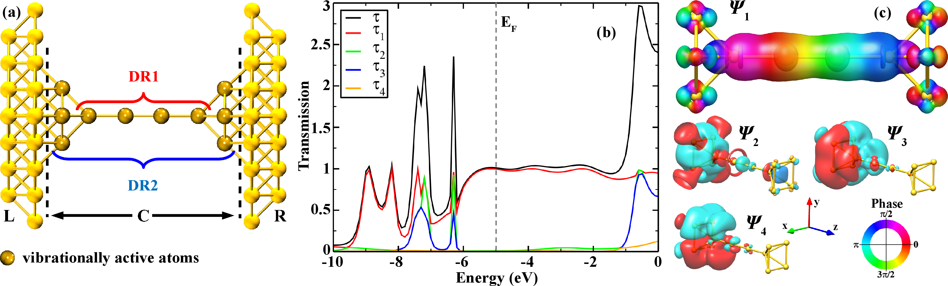
Figure 1: (a) Chain of four Au atoms connected to Au electrodes. All atoms in the C region have been relaxed. The dynamical regions, where atoms can vibrate, are marked as DR1 and DR2. (b) Energy-dependent transmission $\tau(E)$ and the four largest transmission probabilities $\tau_{1}(E)$ to $\tau_{4}(E)$ of the eigenchannels. The Fermi energy $E_{\text{F}}$ is indicated by a vertical dashed line. (c) Wavefunctions $\Psi_{1}$ to $\Psi_{4}$ of the corresponding, left-incoming transmission eigenchannels, evaluated at the Fermi energy. The isosurface value is 0.012 $\text{\AA}^{-3/2}$ for $\Psi_{1}$ and 0.004 $\text{\AA}^{-3/2}$ for $\Psi_{2}$ to $\Psi_{4}$.

To test and validate the transport method, we examine a four-atom gold chain. It is connected to two Au $\langle 100\rangle$ electrodes, each consisting of 45 atoms, as shown in Fig. 1a. We started from an ideal geometry, constructed using a lattice constant of $a=4.08$ Å. Then, the C region, consisting of the four chain atoms and the closest four atoms of each electrode (see Fig. 1a), was fully relaxed, while the other atoms in the L and R parts were kept fixed at their ideal face-centered cubic Bravais lattice positions. This system has already been studied with respect to its elastic conductance [68, 69, 70], transmission eigenchannel wavefunctions [58], and inelastic signatures in the current-voltage characteristics due to the EV coupling [35]. It therefore serves as an ideal test system for our newly developed method.

In Fig. 1b the elastic transmission $\tau$ and the four largest transmission eigenchannel probabilities, $\tau_{1}$ to $\tau_{4}$, are displayed as a function of energy. In agreement with previous studies [42, 68, 69, 70] we find that $\tau(E)$ is roughly constant around the Fermi energy $E_{\text{F}}=-5.0$ eV and close to 1 for energies between $-5.5$ and $-2.0$ eV. The peaks occurring between $-8.0$ and $-6.0$ eV are due to Au $d$ states. Consistent with experimental results [71, 72, 73], we obtain a conductance of $G=1.01G_{0}$. The channel decomposition of the transmission shows that at $E_{\text{F}}$ the transport is carried by one almost completely transparent channel with $\tau_{1}=0.996$. The corresponding, left-incoming eigenchannel wavefunction $\Psi_{1}$ in Fig. 1c is evaluated at $E_{\text{F}}$, using the procedure described in Ref. [59]. It possesses rotational symmetry in the transport direction along the chain, which is assumed to coincide with the $z$ axis. Due to this $\sigma$ symmetry, $\Psi_{1}$ is mainly formed from the $s$ and $p_{z}$ valence orbitals of the Au atoms. The phase-factor is color-coded onto the isosurface of the wavefunction. We observe that it changes continuously along the transport direction, as expected for a propagating wave. The next three transmission channels with $\tau_{2}=0.009$, $\tau_{3}=0.003$ and $\tau_{4}=0.003$ arise from tails of transmission resonances of $d$ states around 1.5 eV below $E_{\text{F}}$. These eigenchannels constitute evanescent waves, decaying along the chain. For this reason, we can choose the phase-factors such that the wave-functions $\Psi_{2}$ to $\Psi_{4}$ are purely real in that region. Figure 1c visualizes the $d$ character of the wavefunctions on the Au chain. The wavefunction $\Psi_{2}$ of the second channel is mainly attributed to $d_{3\text{z}^{2}\text{-r}^{2}}$ states with $\sigma$ symmetry along the transport direction. Channels three and four of $\pi$ symmetry are almost degenerate at $E_{\text{F}}$ and their wavefunctions are formed from Au chain $d_{\text{xz}}$ and $d_{\text{yz}}$ orbitals, respectively. The channels involving the remaining two $d$ states, $d_{\text{xy}}$ and $d_{\text{x}^{2}\text{-y}^{2}}$, have a much smaller transmission and are not shown here.

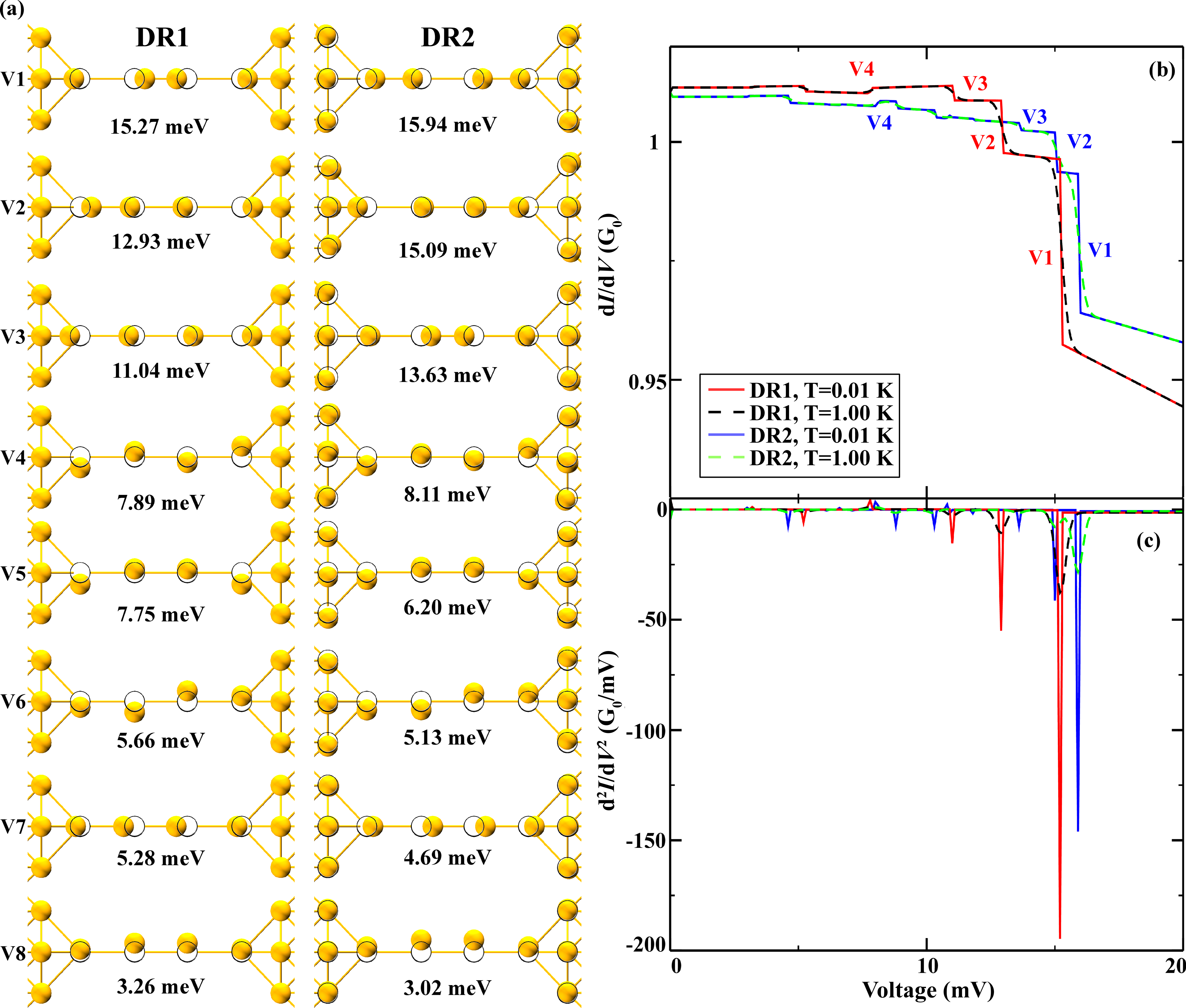
Figure 2: (a) Vibrational modes for DR1 and DR2 with the dynamical regions defined as shown in Fig. 1a. For DR2 those modes are displayed, which are mainly localized on the chain and resemble those of DR1. (b) Differential conductance as a function of voltage for DR1 and DR2 at the temperatures of $T=0.01$ and $1.00$ K. (c) First derivative of the differential conductance plotted in (b).

So far we have just considered the energy-dependent transmission of the elastic term, Eq. (25), of the total current in Eq. (24). Now we include additionally the effects due to the EV coupling, as described by Eqs. (26) and (27). More precisely, we determine in the following the influence of vibrations on the electric current in the WBL, using Eqs. (62)-(64).

We have considered two different DRs, where we take the EV interaction into account (see Fig. 1a). In DR1 we include the EV coupling just for the four chain atoms, in DR2 for all Au atoms in the C region. DR1 with the four dynamic atoms yields 12 vibrational modes, while the 12 dynamic atoms in DR2 lead to 36 modes. Figure 2a shows all the vibrations for DR1 (degenerate transversal modes are depicted only once), while we have selected only those for DR2, which resemble the modes of DR1. Despite the relaxation of all the C atoms, the symmetry of the ideal contact is only slightly perturbed. Hence the transverse modes (V4-V6 and V8) remain basically two-fold degenerate. Expanding the vibrationally active region from DR1 to DR2 causes a blue-shift of the frequencies for the four modes with the highest energy (V1-V4). For the other four modes (V5-V8), the frequencies are red-shifted instead. Overall, however, the changes in the frequencies remain relatively small.

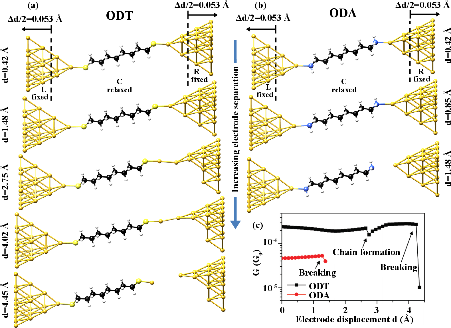
Figure 3: Geometries for (a) ODT and (b) ODA molecules between Au electrodes at different electrode displacements. (c) Evolution of the elastic conductance as a function of the displacement.

The calculated differential conductance as a function of voltage and its derivative are shown in Fig. 2b and 2c for a vibrational broadening of $\eta=0.01$ meV. We observe that the three longitudinal modes (V1-V3) lead to the largest change in the current. Since the longitudinal modes mainly couple to the first transmission channel due to symmetry, they tend to decrease the conductance consistent with the “1/2 rule” [74, 75, 76]. The mode V1 gives rise to the largest decrease of the conductance followed by V2 and V3. Comparing the results for DR1 and DR2, we find that the curves remain very similar, but the signals from V1 to V3 are shifted to higher bias voltages for DR2, as expected from the frequency shifts in Fig. 2a. The additional modes of DR2, which are mainly localized in the electrodes, do not give rise to pronounced signals in the $\mbox{d}I/\mbox{d}V$. The increase in the conductance at energies of the transversal mode V4 is due to its coupling to the low-transmitting, $d$-like channels 3 and 4 [74, 75, 76, 77]. Increasing the temperature from $T=0.01$ to $1.00$ K tends to smear out the sharp steps in the $\mbox{d}I/\mbox{d}V$. All the presented results for DR1 are in good agreement with previous tight-binding and ab-initio studies [35, 40].

3.2 Single-molecule gold-octane-gold junctions

The electronic and vibrational properties of single-molecule junctions are determined by the electrodes, the contacted molecule and the molecule-electrode interfaces. They are reflected in the IET spectra, which turn out to be a sensitive probe to characterize the junctions. This regards for instance molecule-specific signatures to prove the presence of a particular molecule between the electrodes or sensitivity to geometrical changes during the junction elongation.

In Ref. [28] we analyzed both experimentally and theoretically octanedithiol (ODT) and octanediamine (ODA) single-molecule junctions. The focus was on the properties of the metal-molecule interface, and we showed that the two different anchoring groups give rise to qualitatively different features in the IET spectra. For sulfur anchors, which bind strongly to gold surfaces, the S-Au modes remained approximately constant in energy during the junction elongation. Additionally, we observed IET peaks corresponding to the formation of gold chains. For the much weaker $\text{NH}_{2}\text{-Au}$ bond we found instead a red-shift of the N-Au mode with increasing electrode separation, and chain formation was absent. Here we will extend this work and analyze theoretically in more detail the IET signals related to vibrational modes localized on the molecule.

The ECC for the ODT and ODA junctions is shown in Fig. 3a and 3b. It is divided into the L, C and R regions at the dashed lines indicated for the topmost geometries. The two outermost layers of the Au electrodes are the L and R parts. They are kept fixed at their ideal face-centered cubic lattice positions, while the inner part or C region is relaxed to its ground-state geometry. The vibrationally active region is identical to C. To simulate an adiabatic stretching of the molecular junctions, we proceed as described in Ref. [28]. The electrodes to the left and the right are separated symmetrically by $\Delta d=0.2\>\text{a.u.}\approx 0.106\>\text{\text{\AA}}$ in each step. In Fig. 3a and 3b selected stages of the stretching process are displayed, and the elastic conductance for each electrode separation is summarized in Fig. 3c. For ODA the dependence of the conductance on the electrode separation is rather weak, showing a slight increase until the contact breaks at $d=1.48$ Å. The overall length of the conductance plateau for ODT is much longer than for ODA and the conductance-distance trace exhibits several distinct features: At first the conductance remains roughly constant before a kink appears at $d=2.75$ Å. It coincides with a plastic deformation of the contact, resulting in the formation of a gold chain (see Fig. 3a). Before the contact breaks at $d=4.34$ Å, the conductance increases with $d$ roughly to its starting value at $d=0$. For a more detailed discussion we refer to our previous work in Ref. [28].

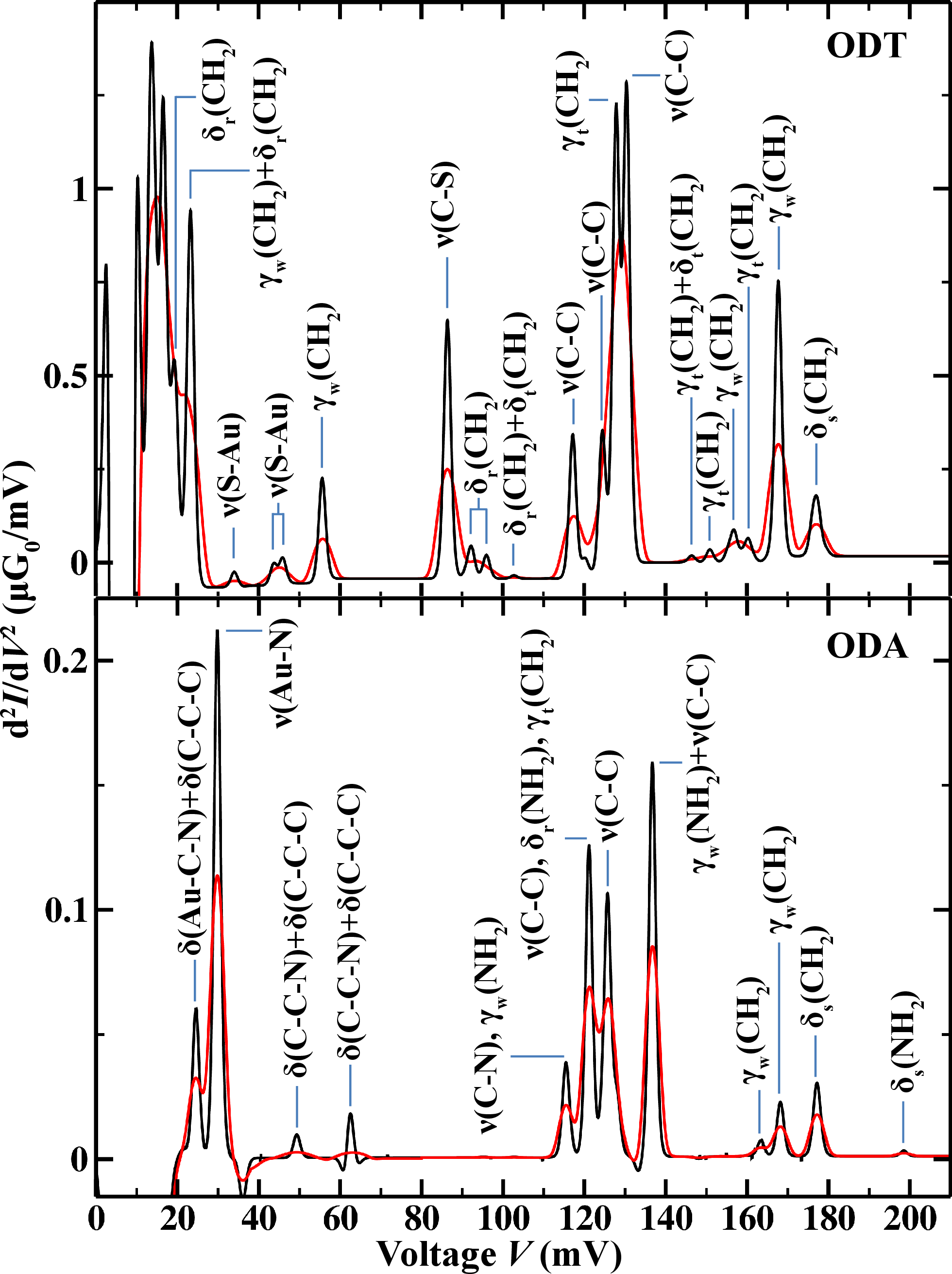
Figure 4: IET spectra without (black curve) and with (red curve) lock-in broadening for ODT and ODA. When we separate modes by a comma, there are several contributing to the same peak. When we use “$+$”, a single mode has a mixed character.

Next, we discuss inelastic effects in electrical transport due to the EV coupling by considering the IET spectra of the ODT and ODA junctions. We use the same terminology for the modes as in our Ref. [28] and refer the interested reader to that work for its detailed description. We note that the characterization of the vibrations in terms of molecule-internal modes remains approximate due to the absence of molecular symmetries in the junctions. As compared to Ref. [28], we focus here mainly on the vibrational modes of the octane molecules that do not involve the Au electrodes.

For all the IET spectra, calculated within the WBL, we assumed a temperature of $T=4.2$ K and a vibrational broadening of $\eta=1$ meV. They describe the intrinsic line-width broadening of the IET signals due to a finite temperature and finite life-time of the vibrational modes, respectively. In the experiments, the lock-in measurement technique constitutes another source of broadening. It can be accounted for by convoluting the $\mbox{d}^{2}I/\mbox{d}V^{2}$ with an instrumental function, which depends on the modulation voltage $V_{\omega}$, applied to detect the IET characteristics [78, 79]. In Fig. 4 the effect of this broadening on the IET spectra is demonstrated for $V_{\omega}=5$ mV, the modulation voltage used in Ref. [28]. The additional smearing may prevent experimental resolution of individual vibrational modes, if they are very close in energy. Even if the lock-in broadening is important for the comparison of calculated IET spectra and measured ones, we neglect it in the following calculations, as we did for the Au junctions above. In this way we finely resolve all the vibrational features and consider only the intrinsic broadening effects.

The electron-phonon coupling in ODT junctions has already been the subject of several previous experimental [24, 27, 28, 80, 81] and theoretical [82, 83, 84] studies. Our calculated vibrational frequencies and IET spectra are consistent with these works. The IET spectra for ODT and ODA, displayed in Fig. 4, are for a stretching distance of $d=0.42$ Å, where the molecules adopt a rather straight configuration inside the junctions. At that $d$, the bond lengths $d_{\text{C-C}}$ and bond angles $\alpha_{\text{C-C-C}}$ are very similar for ODT and ODA.

When we compare the IET spectra at high energies from $145$ to $200$ meV, we find that the positions of the pronounced peaks stemming from $\gamma_{\text{w}}(\text{CH}_{2})$ and $\delta_{\text{s}}(\text{CH}_{2})$ modes, located at 169 and 178 meV, respectively, are the same for ODT and ODA. The position of the second $\gamma_{\text{w}}(\text{CH}_{2})$ mode at 156 meV for ODT and 163 meV for ODA differs slightly. For ODT we observe small signals from $\gamma_{\text{t}}(\text{CH}_{2})$ modes at 150 and 160 meV as well as a $\gamma_{\text{t}}(\text{CH}_{2})\mbox{+}\delta_{\text{t}}(\text{CH}_{2})$ mode at 145 meV, which are absent for ODA. The very faint signal at $197$ meV can be attributed to a $\delta_{\text{s}}(\text{NH}_{2})$ vibration of the ODA anchoring group. Between $110$ and $145$ meV, $\nu(\text{C-C})$ modes give rise to prominent features in the IET spectra. We can identify three major peaks at slightly different energies. For ODT the $\nu{(\text{C-C})}$ mode with the highest energy is located at $131$ meV, while it is slightly blue-shifted to $137$ meV for ODA and contains an additional $\gamma_{\text{w}}(\text{NH}_{2})$ contribution. At $125$ meV we observe a clear $\nu{(\text{C-C})}$ mode for both anchoring groups. The third $\nu{(\text{C-C})}$ mode is located at $118$ meV for ODT and at a slightly higher energy of $121$ meV for ODA. While the $\nu{(\text{C-C})}$ modes with the highest and lowest energies are blue-shifted for ODA as compared to ODT, the $\gamma_{\text{t}}(\text{CH}_{2})$ mode is red-shifted and located at $128$ meV for ODT and $121$ meV for ODA. Not considering modes with a mixed character, we find three signals involving the N atom of the amino anchoring groups in the energy range: One $\delta_{\text{r}}(\text{NH}_{2})$ mode at $121$ meV and two modes $\nu(\text{C-N})$, $\gamma_{\text{w}}(\text{NH}_{2})$ at $116$ meV. Between $70$ and $110$ meV there are no signatures of vibrational modes present in the IET spectra for ODA. ODT on the other hand shows some small signals belonging to $\delta_{\text{r}}(\text{CH}_{2})$ and $\delta_{\text{t}}(\text{CH}_{2})$ vibrations between $90$ and $105$ meV. The magnitude of these two IET signals is known to depend crucially on the precise contact geometry [83]. In contrast, the $\nu(\text{C-S})$ mode at $86$ meV gives rise to a dominant peak. At energies below $70$ meV, the IET spectra of ODT and ODA differ substantially. In that range we observe most of the modes involving the anchoring groups and the Au electrodes. Additionally, we observe several $\delta(\text{C-C-C})$ and $\delta(\text{C-C-N})$ stretching modes for ODA and some low-energy $\gamma_{\text{w}}(\text{CH}_{2})$ and $\delta_{\text{r}}(\text{CH}_{2})$ modes for ODT. The modes at very low energies are mainly localized on the Au electrodes and shall not be discussed here. Our results confirm that the characteristic peaks in the IET spectra and their sensitivity to the precise contact geometry can be used to infer the precise binding geometry and to distinguish between ODT and ODA, i.e. molecules that differ only in their anchoring group [28].

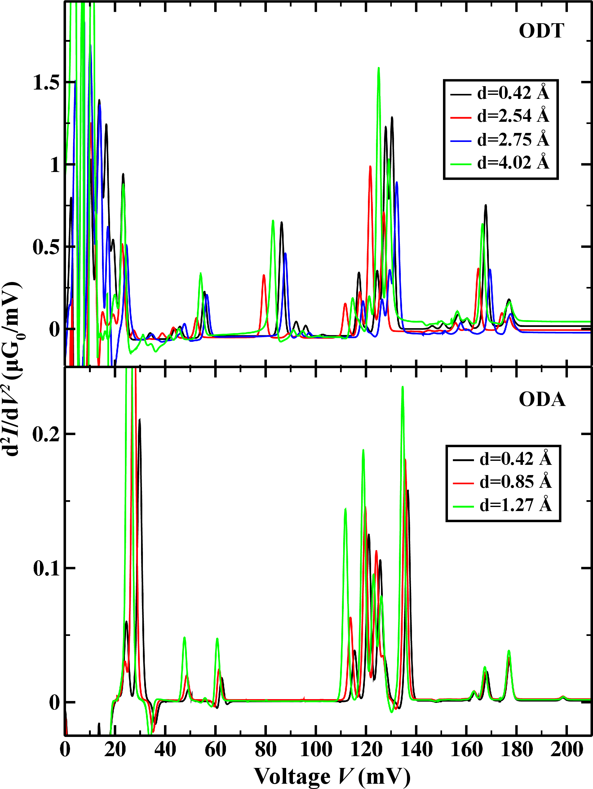
Figure 5: IET spectra for different electrode displacements of the ODT and ODA junctions.

The evolution of the IET spectra with increasing electrode separation is displayed in Fig. 5 for both ODT and ODA. Increasing $d$, increases $d_{\text{C-C}}$ and $\alpha_{\text{C-C-C}}$ in the octane molecule. This affects mainly vibrational modes involving the carbon backbone. For ODA the $\delta(\text{C-C-C})$, $\delta(\text{C-C-N})$ and $\nu(\text{C-C})$ modes are red-shifted by around $3$ meV. The red-shifts occurs continuously during the stretching process from $d=0$ until the contract breaks at $d=1.38$ Å. The energy of the modes involving the ${\text{NH}_{2}}$ anchoring group [$\delta_{s}(\text{NH}_{2})$] and the $\text{CH}_{2}$ units [$\gamma_{\text{w}}(\text{CH}_{2})$, $\delta_{\text{s}}(\text{CH}_{2})$] remains basically constant. As expected, they are not influenced by the mechanical stretching. For ODT a similar behavior is observed, but the plastic deformation of the Au electrodes needs to be taken into account. From $d=0$ to $d=2.54$ Å the ODT contact is elastically deformed, building up stress in the molecule. As for ODA, $d_{\text{C-C}}$ and $\alpha_{\text{C-C-C}}$ are increased, resulting in a red-shift of $\nu(\text{C-C})$ modes by around $7$ to $9$ meV. For the modes with clear $\text{CH}_{2}$ character, the red-shift is smaller and does not exceed $3$ meV. The plastic deformation of the Au electrode, occurring at around $d=2.75$ Å, releases the stress and allows $d_{\text{C-C}}$ and $\alpha_{\text{C-C-C}}$ to restore their initial values. This results in a blue-shift of the vibrational modes which take values slightly above their initial energy. The movement of the peaks in the IET spectra in the subsequent elastic stage until contact rupture is similar to the first one.

4 Conclusions

We presented a new first-principles approach to study the IET spectra of atomic and molecular contacts. To achieve this, we extended the quantum chemistry software package TURBOMOLE to compute the EV couplings via an efficient and accurate semi-analytical derivative scheme based on DFPT. This functionality will be available in TURBOMOLE 6.6. It allows us to describe the coupled system of electrons and phonons of the nanostructures at the level of DFT without free parameters. Using a LOE in terms of the EV coupling [40], we determined the influence of vibrations on the electrical current. This constitutes an important extension of our previous capabilities to study the elastic transport properties of nanoscale conductors [42]. Gold electrodes bridged by an atomic chain served as test system and demonstrated that our approach is consistent with experimental and theoretical studies in the literature.

Based on these theoretical developments, we studied the IET spectra of ODT and ODA single-molecule junctions. We extended our previous investigations in Ref. [28], where we focused on the metal-molecule interface, by a more detailed discussion of the molecular vibrations localized on the octane itself. We found that the vibrations of the alkane backbone differ only slightly for the two different anchoring groups. However, anchoring-group-specific modes could be clearly resolved in the IET spectra, offering the possibility to distinguish between ODT and ODA. The sulfur and amine anchors differ substantially in their binding strength to Au. This resulted in a qualitatively different behavior of the junctions during their elongation. While the ODA junction broke at the weak Au-N bond, gold electrodes were plastically deformed for ODT. Ultimately, the ODT junction ruptured at a Au-Au bond and not the strong Au-S bond. During the junction elongation we observed a red-shift of $\delta(\text{C-C-C})$ and $\nu(\text{C-C})$ modes for both anchoring groups due to the increasing bond lengths $d_{\text{C-C}}$ and bond angles $\alpha_{\text{C-C-C}}$. The methylene vibrations on the other hand were only slightly affected by the increasing electrode separation. For ODT the plastic deformation of the Au electrodes was reflected also in the molecular vibrations. Due to the relaxation of the stress built up during elastic stages, the plastic deformation lead to a decrease of $d_{\text{C-C}}$ and $\alpha_{\text{C-C-C}}$, blue-shifting the corresponding vibrational modes. Subsequent elastic deformations decreased their energies again.

So far, heating effects and the non-equilibrium distribution of the phonons are taken into account in an approximate way in our ab-initio calculations. The consideration of the coupling of the vibrations in the central device region to those in the electrodes [85, 86] constitutes a natural extension of the developed methodology. Work along these lines combined with calculations for a larger set of atomic and molecular junctions will allow new insights into the interaction of electrons and phonons, important for challenges such as the improved control of electron transport and heating in electronic nanocircuits.

We thank Y. Kim for his contributions to the experimental work in Ref. [28], J. C. Cuevas for stimulating discussions, and the TURBOMOLE GmbH for providing us with the source code of TURBOMOLE. The work of M.B. was supported through the DFG priority program 1243 and a FY2012 (P12501) Postdoctoral Fellowship for Foreign Researchers from the Japan Society for Promotion of Science (JSPS) as well as by a JSPS KAKENHI, i.e., “Grant-in-Aid for JSPS Fellows”, Grant No. 24$\cdot$02501. In addition, J.K.V. gratefully acknowledges funding through the Academy of Finland, T.J.H. through the Baden-Württemberg Stiftung within the Research Network of Excellence “Functional Nanostructures”, E.S. through the DFG via SPP 1243 and SFB 767, G.S. through the Initial Training Network “NanoCTM” (Grant No. FP7-PEOPLE-ITN-2008-234970), and F.P. through the DFG Center for Functional Nanostructures (Project C3.6) and the Carl Zeiss foundation.

References

- [1] N. Agraït, A. L. Yeyati, and J. M. van Ruitenbeek, Phys. Rep. 377, 81 (2003).
- [2] J. C. Cuevas and E. Scheer, Molecular Electronics (World Scientific Publishing Company, Singapore, 2010).
- [3] M. Ratner, Nat. Nanotechnol. 8, 378 (2013).
- [4] M. Galperin, M. A. Ratner, and A. Nitzan, J. Phys.: Condens. Matter 19, 103201 (2007).
- [5] Z. Ioffe, T. Shamai, A. Ophir, G. Noy, I. Yutsis, K. Kfir, O. Cheshnovsky, and Y. Selzer, Nat. Nanotechnol. 3, 727 (2008).
- [6] D. R. Ward, D. A. Corley, J. M. Tour, and D. Natelson, Nat. Nanotechnol. 6, 33 (2011).
- [7] W. Lee, K. Kim, W. Jeong, L. A. Zotti, F. Pauly, J. C. Cuevas, and P. Reddy, Nature 498, 209 (2013).
- [8] M. Jonson and G. D. Mahan, Phys. Rev. B 21, 4223 (1980).
- [9] M. Jonson and G. D. Mahan, Phys. Rev. B 42, 9350 (1990).
- [10] J. M. Ziman, Electrons and Phonons (Oxford University Press, Oxford, 2001).
- [11] L. Luo, S. H. Choi, and C. D. Frisbie, Chem. Mater. 23, 631 (2011).
- [12] Z. Yao, C. L. Kane, and C. Dekker, Phys. Rev. Lett. 84, 2941 (2000).
- [13] P. G. Collins, M. Hersam, M. Arnold, R. Martel, and P. Avouris, Phys. Rev. Lett. 86, 3128 (2001).
- [14] H. Park, A. K. L. Lim, A. P. Alivisatos, J. Park, and P. L. McEuen, Appl. Phys. Lett. 75, 301 (1999).
- [15] R. H. M. Smit, C. Untiedt, and J. M. van Ruitenbeek, Nanotechnology 15, S472 (2004).
- [16] T. Taychatanapat, K. I. Bolotin, F. Kuemmeth, and D. C. Ralph, Nano Lett. 7, 652 (2007).
- [17] H. B. Heersche, G. Lientschnig, K. O’Neill, H. S. J. van der Zant, and H. W. Zandbergen, Appl. Phys. Lett. 91, 072107 (2007).
- [18] C. Schirm, M. Matt, F. Pauly, C. J. Cuevas, P. Nielaba, and E. Scheer, Nat. Nanotechnol. 8, 645 (2013).
- [19] B. C. Stipe, M. A. Rezaei, and W. Ho, Science 280, 1732 (1998).
- [20] R. H. M. Smit, Y. Noat, C. Untiedt, N. D. Lang, M. C. van Hemert, and J. M. van Ruitenbeek, Nature 419, 906 (2002).
- [21] D. Djukic, K. S. Thygesen, C. Untiedt, R. H. M. Smit, K. W. Jacobsen, and J. M. van Ruitenbeek, Phys. Rev. B 71, 161402 (2005).
- [22] N. Agraït, C. Untiedt, G. Rubio-Bollinger, and S. Vieira, Phys. Rev. Lett. 88, 216803 (2002).
- [23] J. G. Kushmerick, J. Lazorcik, C. H. Patterson, R. Shashidhar, D. S. Seferos, and G. C. Bazan, Nano Lett. 4, 639 (2004).
- [24] W. Wang, T. Lee, I. Kretzschmar, and M. A. Reed, Nano Lett. 4, 643 (2004).
- [25] M. Paulsson, T. Frederiksen, and M. Brandbyge, Nano Lett. 6, 258 (2006).
- [26] M. Kiguchi, O. Tal, S. Wohlthat, F. Pauly, M. Krieger, D. Djukic, J. C. Cuevas, and J. M. van Ruitenbeek, Phys. Rev. Lett. 101, 046801 (2008).
- [27] C. R. Arroyo, T. Frederiksen, G. Rubio-Bollinger, M. Vélez, A. Arnau, D. Sánchez-Portal, and N. Agraït, Phys. Rev. B 81, 075405 (2010).
- [28] Y. Kim, T. J. Hellmuth, M. Bürkle, F. Pauly, and E. Scheer, ACS Nano 5, 4104 (2011).
- [29] C. Caroli, R. Combescot, P. Nozieres, and D. Saint-James, J. Phys. C 5, 21 (1972).
- [30] N. Lorente, M. Persson, L. J. Lauhon, and W. Ho, Phys. Rev. Lett. 86, 2593 (2001).
- [31] J. Koch and F. von Oppen, Phys. Rev. Lett. 94, 206804 (2005).
- [32] M. Galperin, A. Nitzan, and M. A. Ratner, Phys. Rev. B 73, 045314 (2006).
- [33] S. Y. Quek, L. Venkataraman, H. J. Choi, S. G. Louie, M. S. Hybertsen, and J. B. Neaton, Nano Lett. 7, 3477 (2007).
- [34] M. Strange and K. S. Thygesen, Beilstein J. Nanotechnol. 2, 746 (2011).
- [35] T. Frederiksen, M. Paulsson, M. Brandbyge, and A. P. Jauho, Phys. Rev. B 75, 205413 (2007).
- [36] W. Koch and M. C. Holthausen, A Chemist’s Guide to Density Functional Theory (Wiley-VCH, Weinheim, 2001).
- [37] R. M. Martin, Electronic Structure: Basic Theory and Practical Methods (Cambridge University Press, Cambridge, 2008).
- [38] S. Baroni, S. de Gironcoli, A. Dal Corso, and P. Giannozzi, Rev. Mod. Phys. 73, 515 (2001).
- [39] Y. Asai, Phys. Rev. Lett. 93, 246102 (2004).
- [40] J. K. Viljas, J. C. Cuevas, F. Pauly, and M. Häfner, Phys. Rev. B 72, 245415 (2005).
- [41] E. J. McEniry, T. Frederiksen, T. N. Todorov, D. Dundas, and A. P. Horsfield, Phys. Rev. B 78, 035446 (2008).
- [42] F. Pauly, J. K. Viljas, U. Huniar, M. Häfner, S. Wohlthat, M. Bürkle, J. C. Cuevas, and G. Schön, New J. Phys. 10, 125019 (2008).
- [43] H. F. Schaefer III and Y. Yamaguchi, J. Mol. Struct. 135, 369 (1986).
- [44] W. Kohn and L. J. Sham, Phys. Rev. 140, A1133 (1965).
- [45] P. Hohenberg and W. Kohn, Phys. Rev. 136, B864 (1964).
- [46] R. G. Parr and W. Yang, Annu. Rev. Phys. Chem. 46, 701 (1995).
- [47] C. Fiolhais, F. Nogueira, and M. A. L. Marques, A Primer in Density Functional Theory (Springer, Berlin, 2003).
- [48] K. Capelle, Braz. J. Phys. 36, 1318 (2006).
- [49] M. A. L. Marques, C. A. Ullrich, F. Nogueira, A. Rubio, K. Burke, and E. K. U. Gross, Time-Dependent Density Functional Theory (Springer, Berlin, 2006).
- [50] TURBOMOLE V6.3, TURBOMOLE GmbH Karlsruhe, http://www.turbomole.de. TURBOMOLE is a development of University of Karlsruhe and Forschungszentrum Karlsruhe 1989-2007, TURBOMOLE GmbH since 2007.
- [51] P. Deglmann, F. Furche, and R. Ahlrichs, Chem. Phys. Lett. 362, 511 (2002).
- [52] J. A. Pople, R. Krishnan, H. B. Schlegel, and J. S. Binkley, Int. J. Quantum Chem. 16, 225 (1979).
- [53] S. Baroni, P. Giannozzi, and A. Testa, Phys. Rev. Lett. 58, 1861 (1987).
- [54] B. G. Johnson and M. J. Fisch, J. Chem. Phys. 100, 7429 (1994).
- [55] X. Gonze, Phys. Rev. A 52, 1086 (1995).
- [56] P. Deglmann, K. May, F. Furche, and R. Ahlrichs, Chem. Phys. Lett. 384, 103 (2004).
- [57] A. Komornicki, K. Ishida, K. Morokuma, R. Ditchfield, and M. Conrad, Chem. Phys. Lett. 45, 595 (1977).
- [58] M. Paulsson and M. Brandbyge, Phys. Rev. B 76, 115117 (2007).
- [59] M. Bürkle, J. K. Viljas, D. Vonlanthen, A. Mishchenko, G. Schön, M. Mayor, T. Wandlowski, and F. Pauly, Phys. Rev. B 85, 075417 (2012).
- [60] P. Hyldgaard, S. Hershfield, J. Davies, and J. Wilkins, Ann. Phys. 236, 1 (1994).
- [61] L. K. Dash, H. Ness, and R. W. Godby, J. Chem. Phys. 132, 104113 (2010).
- [62] A. D. Becke, Phys. Rev. A 38, 3098 (1988).
- [63] J. P. Perdew, Phys. Rev. B 33, 8822 (1986).
- [64] A. Schäfer, H. Horn, and R. Ahlrichs, J. Chem. Phys. 97, 2571 (1992).
- [65] K. Eichkorn, O. Treutler, H. Öhm, M. Häser, and R. Ahlrichs, Chem. Phys. Lett. 242, 652 (1995).
- [66] K. Eichkorn, F. Weigend, O. Treutler, and R. Ahlrichs, Theor. Chem. Acc. 97, 119 (1997).
- [67] D. Andrae, U. Häußermann, M. Dolg, H. Stoll, and H. Preuß, Theor. Chim. Acta 77, 123 (1990).
- [68] J. L. Mozos, P. Ordejón, M. Brandbyge, J. Taylor, and K. Stokbro, Nanotechnology 13, 346 (2002).
- [69] M. Brandbyge, J. L. Mozos, P. Ordejón, J. Taylor, and K. Stokbro, Phys. Rev. B 65, 165401 (2002).
- [70] Y. J. Lee, M. Brandbyge, M. J. Puska, J. Taylor, K. Stokbro, and R. M. Nieminen, Phys. Rev. B 69, 125409 (2004).
- [71] H. Ohnishi, Y. Kondo, and K. Takayanagi, Nature 395, 780 (1998).
- [72] A. I. Yanson, G. Rubio Bollinger, H. E. van den Brom, N. Agraït, and J. M. van Ruitenbeek, Nature 395, 783 (1998).
- [73] R. H. M. Smit, C. Untiedt, A. I. Yanson, and J. M. van Ruitenbeek, Phys. Rev. Lett. 87, 266102 (2001).
- [74] M. Paulsson, T. Frederiksen, and M. Brandbyge, Phys. Rev. B 72, 201101 (2005).
- [75] L. de la Vega, A. Martín-Rodero, N. Agraït, and A. L. Yeyati, Phys. Rev. B 73, 075428 (2006).
- [76] M. Paulsson, T. Frederiksen, H. Ueba, N. Lorente, and M. Brandbyge, Phys. Rev. Lett. 100, 226604 (2008).
- [77] T. Böhler, A. Edtbauer, and E. Scheer, New J. Phys. 11, 013036 (2009).
- [78] J. Klein, A. Léger, M. Belin, D. Défourneau, and M. J. L. Sangster, Phys. Rev. B 7, 2336 (1973).
- [79] P. K. Hansma, Phys. Rep. 30, 145 (1977).
- [80] T. Lee, W. Wang, and M. A. Reed, Jpn. J. Appl. Phys. 44, 523 (2005).
- [81] N. Okabayashi, Y. Konda, and T. Komeda, Phys. Rev. Lett. 100, 217801 (2008).
- [82] A. Pecchia, A. Di Carlo, A. Gagliardi, S. Sanna, T. Frauenheim, and R. Gutierrez, Nano Lett. 4, 2109 (2004).
- [83] G. C. Solomon, A. Gagliardi, A. Pecchia, T. Frauenheim, A. Di Carlo, J. R. Reimers, and N. S. Hush, J. Chem. Phys. 124, 094704 (2006).
- [84] M. Paulsson, C. Krag, T. Frederiksen, and M. Brandbyge, Nano Lett. 9, 117 (2009).
- [85] G. Romano, A. Pecchia, and A. D. Carlo, J. Phys.: Condens. Matter 19, 215207 (2007).
- [86] M. Engelund, M. Brandbyge, and A. P. Jauho, Phys. Rev. B 80, 045427 (2009).