Routing Directions: Keeping it Fast and Simple

Abstract

The problem of providing meaningful routing directions over road networks is of great importance. In many real-life cases, the fastest route may not be the ideal choice for providing directions in written/spoken text, or for an unfamiliar neighborhood, or in cases of emergency. Rather, it is often more preferable to offer “simple” directions that are easy to memorize, explain, understand or follow. However, there exist cases where the simplest route is considerably longer than the fastest. This paper tries to address this issue, by finding near-simplest routes which are as short as possible and near-fastest routes which are as simple as possible. Particularly, we focus on efficiency, and propose novel algorithms, which are theoretically and experimentally shown to be significantly faster than existing approaches.

1 Introduction

Finding the fastest route on road networks has received a renewed interest in the recent past, thanks in large part to the proliferation of mobile location-aware devices. However, there exist many real-life scenarios in which the fastest route may not be the ideal choice when providing routing directions.

As a motivating example, consider the case of a tourist asking for driving directions to a specific landmark. Since the tourist may not be familiar with the neighborhood, it makes more sense to offer directions that involve as few turns as possible, instead of describing in detail an elaborate fastest route. As another example, consider an emergency situation, e.g., natural disaster, terrorist attack, which requires an evacuation plan to be communicated to people on the site. Under such circumstances of distress and disorganization, it is often desirable to provide concise, easy to memorize, and clear to follow instructions.

In both scenarios, the simplest route may be more preferable than the fastest route. As per the most common interpretation [21], turns (road changes) are assigned costs, and the simplest route is the one that has the lowest total turn cost, termed complexity. For simplicity, in the remainder of this work, we assume that all turns have equal cost equal to 1; the generalization to non-uniform costs is straightforward.

In some road networks, the simplest and the fastest route may be two completely different routes. Consider for example a large city, e.g., Paris, that has a large ring road encircling a dense system of streets. The simplest route between two nodes that lie on (or are close to) the ring, would be to follow the ring. On the other hand, the fastest route may involve traveling completely within the enclosing ring. As a result the length of the simplest route can be much larger than that of the fastest route, and vice versa.

Surprisingly, with the exception of [13], the trade-off between length and complexity in finding an optimal route has not received sufficient attention. Our work addresses this issue by studying the problem of finding routes that are as fast and as simple as possible.

In particular, we first study the fastest simplest problem, i.e., of finding the fastest among all simplest routes, which was the topic of [13]. We show that although, for this problem, a label-setting method (a variant of the basic Dijkstra’s algorithm) cannot be directly applied on the road network, it is possible to devise a conceptual graph on which it can. In fact, our proposed algorithm is orders of magnitude faster than the baseline solution. Moreover, using a similar methodology, it is possible to efficiently solve the simplest fastest problem.

Subsequently, we investigate the length-complexity trade-off and introduce two novel problems that relax the constraint that the returned routes must be either fastest or simplest. The fastest near-simplest problem is to find the fastest possible route whose complexity is not more than $1+\epsilon$ times larger than that of the simplest route. On the other hand, the simplest near-fastest problem is to find the simplest possible route whose length is not more than $1+\epsilon$ times larger than that of the fastest route.

These near-optimal problems are significantly more difficult to solve compared to their optimal counterparts. The reason is that there cannot exist a principle of optimality, exactly because the requested routes are by definition sub- optimal in length and complexity. Therefore, one must exhaustively enumerate all routes, and only hope to devise pruning criteria to quickly discard unpromising sub-routes.

We propose two algorithms, based on route enumeration, for finding the simplest near-fastest route; their extension for the fastest near-simplest problem is straightforward. The first follows a depth-first search principle in enumerating paths, whereas the second is inspired by A^∗ search. Both algorithms apply elaborate pruning criteria to eliminate from consideration a large number of sub-routes. Our experimental study shows that they run in less than 400 msec in networks of around 80,000 roads and 110,000 intesections.

The remainder of the paper is organized as follows. Section 2 formally defines the problems and reviews related work. Section 3 discusses the fastest simplest, and Section 4 the simplest near-fastest problem. Then, Section 5 presents our experimental study and Section 6 concludes the paper.

2 Preliminaries

Section 2.1 presents the necessary definition, while Section 2.2 reviews relevant literature.

2.1 Definitions

Let $V$ denote a set of nodes representing road intersections. A road $r$ is a sequence of distinct nodes from $V$. Let $R$ denote a set of roads, such that all nodes appear in at least one road, and any pair of consecutive nodes of some road do not appear in any other, i.e., the roads do not have overlapping subsequences. For a node $n\in V$, the notation $R(n)\subseteq R$ represents the non-empty subset of roads that contain $n$. For two consecutive nodes $n_{i}$, $n_{j}$ of some road $r$, the notation $R(n_{i},n_{j})$ is a shorthand for $r$.

Definition 1.

The road network of $R$ is the directed graph $G_{R}(V,E)$, where $V$ is the set of nodes, and $E\subseteq V\!\times\!V$ contains an edge $e_{ij}=(n_{i},n_{j})$ if $n_{i}$, $n_{j}$ are consecutive nodes in some road.

A road network is associated with two cost functions. The length function $L$ assigns to each edge a cost representing its length, i.e., the travel time or distance between them; formally, $L:E\to\mathbb{R}^{+}$ maps each edge $(n_{i},n_{j})$ to the length $L(n_{i},n_{j})$ of the road segment $n_{i}$ to $n_{j}$.

The complexity function $C$ assigns to each turn from road $r_{i}$ to road $r_{j}$ via node $n_{x}$, which lies on both $r_{i}$ and $r_{j}$, the cost of making the turn. Formally, $C:V\!\times\!R\!\times\!R\to\mathbb{R}^{+}$ maps $(n_{x},r_{i},r_{j})$ to complexity $C(n_{x},r_{i},r_{j})$ from $r_{i}$ to $r_{j}$ via $n_{x}$.

A route $\rho=(n_{a},n_{b},\dots)$ is a path on graph $G_{R}$, i.e., a sequence of nodes from $V$, such that for any two consecutive nodes, say $n_{i}$, $n_{j}$, there exists an edge $e_{ij}$ in $E$.

The length $L(\rho)$ of a route $\rho$ is the sum of the lengths for each edge it contains, and represents the total travel time or distance covered along this route; formally,

$$L(\rho)=\sum_{(n_{i},n_{j})\in\rho}L(n_{i},n_{j}).$$ (1)

A route from source $n_{s}$ to target $n_{t}$ is called a fastest route if its length is equal to the smallest length of any route from $n_{s}$ to $n_{t}$. Given a parameter $\epsilon$, a route from $n_{s}$ to $n_{t}$ is called an near-fastest route if its length is at most $(1+\epsilon)$ times that of the fastest route from $n_{s}$ to $n_{t}$.

The complexity $C(\rho)$ of a route $\rho$ is the sum of complexities for each turn it contains; formally

$$C(\rho)=\sum_{(n_{i},n_{j},n_{k})\in\rho}C(n_{j},R(n_{i},n_{j}),R(n_{j},n_{k})),$$ (2)

where $n_{i}$, $n_{j}$, $n_{k}$ are three consecutive nodes in $\rho$, and $R(n_{i},n_{j})$, $R(n_{j},n_{k})$ are the (unique) roads containing segments $(n_{i},n_{j})$ and $(n_{j},n_{k})$, respectively. A route from $n_{s}$ to $n_{t}$ is called a simplest route if its complexity is equal to the lowest complexity of any route from $n_{s}$ to $n_{t}$. Given a parameter $\epsilon$, a route from $n_{s}$ to $n_{t}$ is called a near-simplest route if its complexity is at most $(1+\epsilon)$ times that of the simplest route from $n_{s}$ to $n_{t}$. Note that the complexity of a simplest route can be 0, i.e., when no road changes exist. In this case, all near-simplest routes must also have complexity 0. To address this, one could simply change the definition of complexity to be the number of roads in a route, and thus at least 1. In the remainder of this paper, we ignore this case, and simply use the original definition of complexity.

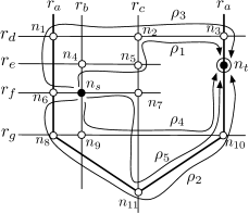
Figure 1: An example road network of seven roads $r_{a}$ – $r_{g}$, where five routes $\rho_{1}$ – $\rho_{5}$ from node $n_{s}$ to $n_{t}$ are depicted.

Table 1: Costs of routes in Figure 1

road	length	complexity	type
$\rho_{1}$	10	4	SF
$\rho_{2}$	40	1	FS
$\rho_{3}$	20	3	SNF ($\epsilon=1$)
$\rho_{4}$	30	2	FNS ($\epsilon=1$)
$\rho_{5}$	40	2	—

This work deals with the following problems. To the best of our knowledge only the first has been studied before in literature [13].

Problem 1. [Fastest Simplest Route] Given a source $n_{s}$ and a target $n_{t}$, find a route that has the smallest length among all simplest routes from $n_{s}$ to $n_{t}$.

Problem 2. [Simplest Fastest Route] Given a source $n_{s}$ and a target $n_{t}$, find a route that has the smallest complexity among all fastest routes from $n_{s}$ to $n_{t}$.

Problem 3. [Fastest Near-Simplest Route] Given a source $n_{s}$ and a target $n_{t}$, find a route that has the smallest length among all near-simplest routes from $n_{s}$ to $n_{t}$.

Problem 4. [Simplest Near-Fastest Route] Given a source $n_{s}$ and a target $n_{t}$, find a route that has the lowest complexity among all near-fastest routes from $n_{s}$ to $n_{t}$.

Note that the first two problems are equivalent to the last two, respectively, if we set $\epsilon=0$. We next present an example illustrating these problems.

Example 1.

Consider the road network of Figure 1 consisting of 7 two-way roads $r_{a}$ – $r_{g}$. Note that all roads have either a north-south or an east-west direction, except road $r_{a}$, which is a ring-road and is thus depicted with a stronger line. The figure also portrays 11 road intersections $n_{1}$–$n_{11}$ with hollow circles, and two special nodes, the source $n_{s}$, drawn with filled circle, and the target $n_{t}$, drawn with a filled circle inside a larger hollow one.

Next, consider five possible routes $\rho_{1}$–$\rho_{5}$ starting from $n_{s}$ and ending at $n_{t}$, which are drawn in Figure 1, and whose lengths and complexities are shown in Table 1. Observe that $\rho_{1}$ is the fastest route from $n_{s}$ to $n_{t}$ with length 10, and, moreover, it has the lowest complexity 4 among all other fastest route (no other exists). Thus, $\rho_{1}$ is the simplest fastest route and the answer to Problem 1.

On the other hand, $\rho_{2}$ is the fastest simplest route and the answer to Problem 1, as it has the lowest complexity 1, following the ring-road to reach the target. But its length, 40, is quite large compared to the other possible routes.

Assume $\epsilon=1$ for the complexity, so that a near-simplest route can have complexity at most twice that of the simplest route, i.e., 2. Observe that two routes $\rho_{4}$ and $\rho_{5}$ are near-simplest. Among them $\rho$ is the fastest, and is thus the answer to Problem 1.

Moreover, assume $\epsilon=1$ for the length as well, so that a near-fastest route can have length at most twice that of the fastest route, i.e., 20. Notice that only $\rho_{3}$ is near-fastest and thus is the answer to Problem 1.

Observe that if we set $\epsilon=2$ for the length, near-fastest routes can have length as large as 30. In this case, $\rho_{3}$ and $\rho_{4}$ are near- fastest, with the latter being the simplest near-fastest. ∎

2.2 Related Work

Dijkstra [7] showed that the fastest route problem exhibits a principle of sub-route optimality and proposed its famous dynamic programming method for finding all fastest routes from a given source. Bi-directional search [17], i.e., initiating two parallel searches from the source and the target can significantly expedite finding the fastest source-to-target route. Since this early work around the 60’s, numerous network preprocessing techniques exist today, including landmarks [11], reach [12], multi-level graphs [20], graph hierarchies [19, 9], graph partitioning [16], labelings [1], and their combinations [2, 3, 6], which are capable of speeding up Dijkstra’s algorithm by orders of magnitude in several instances.

The problem of finding the simplest route was first studied in [5], and more recently in [21, 8]. The basic idea behind these methods, is to construct a pseudo-dual graph of the road network, where road segments become the nodes, the turns between two consecutive road segments become the edges, which are assigned turn costs. Then, finding the simplest route reduces to finding the shortest path on the transformed graph. In contrast, the recent work of [10] solves the simplest route problem directly on the road network. Note that Problem 1 differs with respect to the simplest route problem, as it request a specific simplest route, that with the smallest length. The aforementioned methods return any simplest route.

To the best of our knowledge, only the work in [13] addresses Problem 1, as it proposes a solution that first finds all simplest routes and then selects the fastest among them. The proposed method serves as a baseline approach to our solution for Problem 1 and is detailed in Section 3.1.

Problems 1 and 1 are related to the problem of finding the near-shortest paths on graphs [4, 15]. This paper differs with that line of work in two ways. First, the studied problems involve two cost metrics, length and complexity. Second, their solution is a single route, instead of all possible near-optimal routes.

Problems 1 and 1 are also related to multi-objective shortest path problems (see e.g., [18, 14]), which specify more than one criteria and may return sub-optimal routes. This paper differs with that line of work again in two ways. First, they request a single route. Second, the studied problems introduce a hard constraint on the length or complexity of a solution. Nonetheless, an interesting extension to our work would be to return all routes that capture different length-complexity trade-offs.

3 Fastest Simplest Route

This section discusses Problem 1, and introduces an algorithm that takes advantage of the principle of sub-route optimality to expedite the search. Solving Problem 1 is similar, and thus details are omitted. We first present a recent baseline solution in Section 3.1, and then discuss our approach in Section 3.2.

3.1 Baseline Solution

The work in [13] was the first to address the fact that there can exist multiple simplest routes with greatly varying length, and proposes a solution to finding the fastest among them. This method, which we denote as BSL, operates on a graph that models the intersections of the roads in $R$.

Definition 2.

The intersection graph of $R$ is the undirected graph $G_{I}(R,I)$, where $R$ is the set of roads; and $I\subseteq R\times R\times V$ contains intersection $(n_{x},r_{i},r_{j})$ if $r_{i}\in R(n_{x})$ and $r_{j}\in R(n_{x})$, i.e., node $n_{x}$ belongs to both roads $r_{i}$ and $r_{j}$.

A path on the intersection graph, i.e., a sequence of $R$ vertices such that there exists an intersection in $I$ for any two consecutive vertices in the sequence, is called a road sequence.

BSL finds the fastest simplest route from a source node $n_{s}$ to a target node $n_{t}$. It is based on the observation that a simplest route from $n_{s}$ to $n_{t}$ in the road network is related to a shortest road sequence from a road that contains $n_{s}$ to one that contains $n_{t}$ in the intersection graph. More precisely, BSL operates as follows.

1. For each source road in $R(n_{s})$, find the number of intersections of the shortest road sequence from that source to any of the target roads in $R(n_{t})$, e.g., using a single-source shortest path algorithm on the intersection graph.

2. Determine the smallest number of intersections among those found in the previous step. This number corresponds to the fewest possible intersections in a road sequence that starts from a source and ends at a target road, and is thus equal to the complexity of the simplest route from $n_{s}$ to $n_{t}$ plus 1.

3. Enumerate (e.g., using depth-limited dfs) all road sequences from a source to a target road that have exactly as many intersections as the number determined in the previous step. For each road sequence produced, convert it to a route and determine its length.

4. Select the route with the minimum length, i.e., the fastest, among those produced in the previous step.

3.2 The FastestSimplest Algorithm

The proposed algorithm operates directly on the road network. However, a direct application of a Dijkstra-like (label-setting [7]) method is not possible, because the principle of sub-route optimality does not hold. In particular, this principle suggests that if node $n_{x}$ is in the fastest simplest route from $n_{s}$ to $n_{t}$ then any fastest simplest sub-route from $n_{s}$ to $n_{x}$ can be extended to a fastest simplest route from $n_{x}$ to $n_{t}$. In comparison, it is easy to see that the principle holds for fastest route (shortest paths), as all fastest sub-routes can be extended to fastest routes.

We give a counter-example for the principle of optimality on fastest simplest routes using the road network of Figure 1. Consider the routes $\rho_{2}\!=\!(n_{s},n_{6},n_{8},n_{11},n_{10},n_{t})$ and $\rho_{5}=(n_{s},n_{7},n_{11},n_{10},n_{t})$. The sub-route $\rho_{5}^{\prime}=(n_{s},n_{7},n_{11})$ of $\rho_{5}$ has length 20 and complexity 1, as it involves a single turn from road $r_{f}$ to $r_{c}$ via node $n_{7}$. Similarly, the sub-route $\rho_{2}^{\prime}=(n_{s},n_{6},n_{8},n_{11})$ of $\rho_{2}$ has length 20 and complexity 1, as it involves a single turn from $r_{f}$ to $r_{a}$ via node $n_{6}$. Therefore, both sub-routes are fastest simplest from $n_{s}$ to $n_{11}$. However, the extension of $\rho_{5}^{\prime}$ does not give a fastest simplest route from $n_{s}$ to $n_{t}$; $\rho_{5}$ makes an additional turn at node $n_{11}$ compared to $\rho_{2}$. This violates the principle of optimality for fastest simplest routes.

Therefore, a Dijkstra-like method, which directly exploits this principle of optimality, cannot be applied. For instance, such a method could reach $n_{11}$ first via $r_{c}$ and subsequently ignore any other path reaching $n_{11}$, including the sub-route via $r_{a}$, and thus missing the optimal route from $n_{s}$ to $n_{t}$.

To address the aforementioned lack of sub-route optimality, we construct a conceptual expanded graph, on which the principle optimality holds. Additionally, we show that expanded routes on this graph are uniquely associated with routes on the road network. We emphasize that the expanded graph is only a conceptual structure used for presentation purposes, and that the proposed algorithm does not make use of it as it operates directly on the road network.

Definition 3.

The expanded graph of $G_{R}(V,E)$ is the directed graph $G_{\mathcal{E}}(V^{\prime},E^{\prime})$, where $V^{\prime}\subseteq V\times R$ contains an expanded node $(n_{x},r_{i})$ if $r_{i}\in R(n_{x})$; $E^{\prime}\subseteq V^{\prime}\times V^{\prime}$ contains an edge $((n_{x},r_{i}),(n_{y},r_{j}))$ if $r_{i}\in R(n_{x})$ and $r_{j}\in R(n_{x})$ ($r_{i}$ and $r_{j}$ could be the same road), and additionally $n_{x}$, $n_{y}$ are consecutive nodes in $r_{j}$.

An expanded route $\rho_{\mathcal{E}}=((n_{a},r_{i}),(n_{b},r_{j}),\dots)$ is a path on the expanded graph $G_{\mathcal{E}}$. Each expanded edge can be associated with a length and a turn cost. Therefore, it is possible to define the following costs for an expanded route.

The length $L(\rho_{\mathcal{E}})$ of an expanded route $\rho_{\mathcal{E}}$ is the sum of the lengths associated with each expanded edge; formally,

$$L(\rho_{\mathcal{E}})=\sum_{((n_{x},r_{i}),(n_{y},r_{j}))\in\rho_{\mathcal{E}}}L(n_{x},n_{y}).$$ (3)

Similarly, the complexity $C(\rho_{\mathcal{E}})$ of an expanded route $\rho_{\mathcal{E}}$ is the sum of the turn costs associated with each expanded edge; formally,

$$C(\rho_{\mathcal{E}})=\sum_{((n_{x},r_{i}),(n_{y},r_{j}))\in\rho_{\mathcal{E}}}C(n_{x},r_{i},r_{j}).$$ (4)

An important property regarding the length and complexity of an expanded route is the following. Note that a similar propery does not generally hold for routes on the road network $G_{R}$.

Lemma 1.

Let $\rho_{\mathcal{E}}^{1}$ be an expanded route from $(n_{s},r_{i})$ to $(n_{x},r_{y})$, and $\rho_{\mathcal{E}}^{2}$ be an expanded route from $(n_{x},r_{y})$ to $(n_{t},r_{j})$. If $\rho_{\mathcal{E}}^{1}\rho_{\mathcal{E}}^{2}$ denotes the concatenation of the two expanded routes, then, it holds that $L(\rho_{\mathcal{E}}^{1}\rho_{\mathcal{E}}^{2})=L(\rho_{\mathcal{E}}^{1})+L(\rho_{\mathcal{E}}^{2})$, and $C(\rho_{\mathcal{E}}^{1}\rho_{\mathcal{E}}^{2})=C(\rho_{\mathcal{E}}^{1})+C(\rho_{\mathcal{E}}^{2})$.

Proof.

The proof follows because both the length and complexity functions are defined independently for each expanded edge of an expanded route. ∎

It should be apparent that expanded routes are closely related with (non-expanded) routes. First, let us examine the $G_{R}$ to $G_{\mathcal{E}}$ relationship, which is one to many.

We associate a route $\rho$ from $n_{s}$ to $n_{t}$ on the road network $G_{R}$ to a set $\mathcal{E}(\rho)$ of expanded routes on $G_{\mathcal{E}}$, which only differ in their first and last expanded nodes. Particularly, for an expanded route $\rho_{\mathcal{E}}\in\mathcal{E}(\rho)$, its first expanded node is $(n_{s},r_{i})$, where $r_{i}\in R(n_{s})$, the last expanded node is $(n_{t},r_{j})$, where $r_{j}\in R(n_{t})$, and the $k$-th expanded node (for $k>1$) is $(n_{k},R(n_{k-1},n_{k}))$, where $n_{k-1}$, $n_{k}$ are the $(k\!-\!1)$-th, $k$-th nodes in $\rho$, respectively, and $R(n_{k-1},n_{k})$ is the unique road that contains the edge $(n_{k-1},n_{k})$. Conversely, an expanded route $\rho_{\mathcal{E}}$ is associated with a unique route $\rho$.

Given a route $\rho$, we define the special expanded route of $\rho$, denoted as $\rho_{\mathcal{E}}^{*}$, to be the expanded route in $\mathcal{E}(\rho)$ that has $(n_{s},R(n_{s},n_{s+1}))$ as its first expanded node, and $(n_{t},R(n_{t-1},n_{t}))$ as its last expanded node, where $n_{s+1}$ is the second node in route $\rho$, $R(n_{s},n_{s+1})$ is the unique road containing edge $(n_{s},n_{s+1})$, $n_{t-1}$ is the second-to-last node in route $\rho$, and $R(n_{t-1},n_{t})$ is the unique road containing edge $(n_{t-1},n_{t})$.

An even more important property is the following.

Lemma 2.

The length of a route $\rho$ is equal to the length of any expanded route $\rho_{\mathcal{E}}\in\mathcal{E}(\rho)$. The complexity of a route $\rho$ is equal to the complexity of the special expanded route $\rho_{\mathcal{E}}^{*}\in\mathcal{E}(\rho)$.

Proof.

For convenience, assume that $\rho=(n_{1},n_{2},\dots,n_{t})$. Then, the length of the route is $\displaystyle L(\rho)=\sum_{k=1}^{t-1}L(n_{k},n_{k+1})$, and its complexity is $\displaystyle C(\rho)=\sum_{k=2}^{t-1}C(n_{k},R(n_{k-1},n_{k}),R(n_{k},n_{k+1}))$.

An expanded route of $\rho$ is

$$\rho_{\mathcal{E}}=((n_{1},r_{s}),\dots,(n_{k},R(n_{k-1},n_{k})),\dots,(n_{t},r_{e})),$$

where $r_{s}\in R(n_{1})$ and $r_{e}\in R(n_{t})$. Observe that the length of an expanded route is $L(\rho_{\mathcal{E}})=\sum_{k=1}^{t-1}L(n_{k},n_{k+1})$, which is equal to $L(\rho)$. Hence, the first part of the lemma holds.

The special expanded route of $\rho$ is $\rho_{\mathcal{E}}^{*}=$

$$((n_{1},R(n_{1},n_{2})),\dots,(n_{k},R(n_{k-1},n_{k})),\dots,(n_{t},R(n_{t-1},n_{t}))).$$

The complexity of the special expanded route is

$$C(\rho_{\mathcal{E}}^{*})= \ C(n_{1},R(n_{1},n_{2}),R(n_{1},n_{2}))$$

$$\ +\sum_{k=2}^{t-1}C(n_{k},R(n_{k-1},n_{k}),R(n_{k},n_{k+1}))$$

$$= \ 0+C(\rho),$$

where the first term is zero because the turn cost on the same road is zero. Hence the second part of the lemma also holds. ∎

Next, let us examine the $G_{\mathcal{E}}$ to $G_{R}$ relationship, which is many to one. We associate an expanded route $\rho_{\mathcal{E}}$ from $(n_{s},r_{i})$ to $(n_{t},r_{j})$ to a unique route $\rho=\mathcal{E}^{-1}(\rho_{\mathcal{E}})$ from $n_{s}$ to $n_{t}$ on $G_{R}$, such that the $k$-th node (for any $k$) of $\rho$ is $n_{k}$, where $(n_{k},r_{x})$ is the $k$-th expanded node of $\rho_{\mathcal{E}}$.

Lemma 3.

The length of an expanded route $\rho_{\mathcal{E}}$ is equal to the length of the route $\rho=\mathcal{E}^{-1}(\rho_{\mathcal{E}})$. The complexity of a route $\rho_{\mathcal{E}}$ is not smaller than the complexity of the route $\rho=\mathcal{E}^{-1}(\rho_{\mathcal{E}})$.

Proof.

For convenience, assume that the expanded route is $\rho_{\mathcal{E}}=((n_{1},r_{1}),(n_{2},r_{2}),\dots,(n_{t},r_{t}))$. Then, its length is $\displaystyle L(\rho_{\mathcal{E}})=\sum_{k=1}^{t-1}L(n_{k},n_{k+1})$, and its complexity is $\displaystyle C(\rho_{\mathcal{E}})=\sum_{k=1}^{t-1}C(n_{k},r_{k},r_{k+1})$.

The route on $G_{R}$ is $\rho=\mathcal{E}^{-1}(\rho_{\mathcal{E}})=(n_{1},n_{2},\dots,n_{t})$, and has length $\displaystyle L(\rho)=\sum_{k=1}^{t-1}L(n_{k},n_{k+1})=L(\rho_{\mathcal{E}})$, which proves the first part of the lemma.

The complexity of the non expanded route $\rho$ is

$$C(\rho)= \ \sum_{k=2}^{t-1}C(n_{k},R(n_{k-1},n_{k}),R(n_{k},n_{k+1}))$$

$$= \sum_{k=2}^{t-1}C(n_{k},r_{k},r_{k+1})$$

$$= \sum_{k=1}^{t-1}C(n_{k},r_{k},r_{k+1})-C(n_{1},r_{1},r_{2})$$

$$= C(\rho_{\mathcal{E}})-C(n_{1},r_{1},r_{2})\leq C(\rho_{\mathcal{E}}),$$

since $R(n_{k-1},n_{k})=r_{k}$ and $R(n_{k},n_{k+1})=r_{k+1}$, which proves the second part of the lemma. ∎

We next introduce a lexicographic total order, which applies to routes or expanded routes. Note that in this section, we use this order exclusively for expanded routes. Given two routes $\rho^{1}$, $\rho^{2}$, we say that $\rho^{1}$ is FS-shorter than $\rho^{2}$ and denote as $\rho^{1}<_{FS}\rho^{2}$ if $C(\rho^{1})<C(\rho^{1})$ or if $C(\rho^{1})=C(\rho^{1})$ and $L(\rho^{1})<L(\rho^{1})$. Intuitively, being FS-shorter implies being simpler or as simple but faster.

The following theorem presents an important property regarding this order on expanded routes.

Theorem 1.

Let $\rho^{FS}$ be a fastest simplest route on $G_{R}$ from $n_{s}$ to $n_{t}$, and let $\rho_{\mathcal{E}}^{FS*}$ denote its special expanded route. It holds that there exists no other expanded route that starts from $(n_{s},r_{i})$ and ends at $(n_{t},r_{j})$, for any $r_{i}\in R(n_{s})$ and $r_{j}\in R(n_{t})$ that is FS-shorter than $\rho_{\mathcal{E}}^{FS*}$.

Proof.

We prove by contradiction. Suppose there exists an expanded route $\rho_{\mathcal{E}}^{\prime}$ from $(n_{s},r_{i})$ to $(n_{t},r_{j})$, for some $r_{i}\in R(n_{s})$ and $r_{j}\in R(n_{t})$, such that it is FS-shorter than $\rho_{\mathcal{E}}^{FS*}$. Therefore, one of the two conditions are true:

$$C(\rho_{\mathcal{E}}^{\prime})<C(\rho_{\mathcal{E}}^{FS*}),\text{ or}$$ (5)

$$C(\rho_{\mathcal{E}}^{\prime})=C(\rho_{\mathcal{E}}^{FS*})\text{ and }L(\rho_{\mathcal{E}}^{\prime})<L(\rho_{\mathcal{E}}^{FS*}).$$ (6)

Consider the route $\rho^{\prime}=\mathcal{E}^{-1}(\rho_{\mathcal{E}}^{\prime})$. From Lemma 3, we have that $L(\rho^{\prime})=L(\rho_{\mathcal{E}}^{\prime})$ and $C(\rho^{\prime})\leq C(\rho_{\mathcal{E}}^{\prime})$. Moreover, since $\rho_{\mathcal{E}}^{FS*}$ is the special expanded route of $\rho^{FS}$, we have from Lemma 2 that $L(\rho_{\mathcal{E}}^{FS*})=L(\rho^{FS})$ and $C(\rho_{\mathcal{E}}^{FS*})=C(\rho^{FS})$.

Using these relationships, the two conditions become

$$C(\rho^{\prime})<C(\rho^{FS}),\text{ or}$$ (7)

$$C(\rho^{\prime})=C(\rho^{FS})\text{ and }L(\rho^{\prime})<L(\rho^{FS}),$$ (8)

which imply that $\rho^{\prime}$ is either simpler than $\rho^{FS}$ or as simple but faster. Therefore, $\rho^{FS}$ cannot be a fastest simplest route, which is a contradiction. ∎

Theorem 1 implies that to find a fastest simplest route on $G_{R}$, it suffices to find a FS-shortest expanded route on $G_{\mathcal{E}}$.

The following theorem shows that a principle of optimality holds for FS-shortest expanded routes on $G_{\mathcal{E}}$.

Theorem 2.

Let $\rho_{\mathcal{E}}$ denote an FS-shortest expanded route from $(n_{s},r_{i})$ to $(n_{t},r_{j})$ that passes through $(n_{x},r_{y})$. Furthermore, let $\rho_{\mathcal{E}}^{1}$ denote its sub-route from $(n_{s},r_{i})$ to $(n_{x},r_{y})$, and $\rho_{\mathcal{E}}^{2}$ its sub-route from $(n_{x},r_{y})$ to $(n_{t},r_{j})$. It holds that both $\rho_{\mathcal{E}}^{1}$ and $\rho_{\mathcal{E}}^{2}$ are FS-shortest. Moreover, if $\rho_{\mathcal{E}}^{1^{\prime}}$ is another FS-shortest expanded route from $(n_{s},r_{i})$ to $(n_{x},r_{y})$, then $\rho_{\mathcal{E}}^{1^{\prime}}\rho_{\mathcal{E}}^{2}$ is an FS-shortest expanded route from $(n_{s},r_{i})$ to $(n_{t},r_{j})$.

Proof.

Suppose $\rho_{\mathcal{E}}^{1}$ is not an FS-shortest expanded route from $(n_{s},r_{i})$ to $(n_{x},r_{y})$. Then there exists another expanded route, say $\rho_{\mathcal{E}}^{1*}$, that is FS-shorter. From Lemma 1, it is easy to see that $\rho_{\mathcal{E}}^{1*}\rho_{\mathcal{E}}^{2}$ is FS-shorter than $\rho_{\mathcal{E}}$, which is a contradiction as the latter is FS-shortest. A similar argument holds for $\rho_{\mathcal{E}}^{2}$. Hence the first part of the theorem is proved.

Regarding expanded route $\rho_{\mathcal{E}}^{1^{\prime}}$, observe that since it is FS- shortest it has the same length and complexity with $\rho_{\mathcal{E}}^{1}$. Then by Lemma 1, $\rho_{\mathcal{E}}^{1^{\prime}}\rho_{\mathcal{E}}^{2}$ has the same length and complexity with $\rho_{\mathcal{E}}$. Therefore, it has to be also FS-shortest, which proves the second part of the theorem. ∎

The key point in Theorem 2 is that it holds for any expanded route on $G_{\mathcal{E}}$. In contrast, this does not hold for routes on the road network $G_{R}$, as we have argued in the beginning of this section.

Given Theorem 2, we can apply a Dijkstra’s algorithm, or any variant, to find the FS-shortest expanded route on $G_{\mathcal{E}}$. Then, from Theorem 1, we immediately obtain a fastest simplest route on $G_{R}$.

In what follows, we present the FastestSimplest (FS) algorithm, a label- setting method (a generalization of Dijkstra’s algorithm) for finding a fastest simplest route on $G_{R}$, which operates directly on the road network and constructs directly routes, instead of expanded routes.

The pseudocode of the FS algorithm is depicted in Algorithm 1. Although FS operates on the road network $G_{R}$, it updates labels for expanded nodes. A label $\lambda(n,r)$ for expanded node $(n,r)$ is equal to $\langle n,r|len,cpl,n_{prev},r_{prev}\rangle$ and represents an expanded route from $(n_{s},r_{i})$, for some $r_{i}\in R(n_{s})$, up to $(n,r)$. In particular, $len$, $cpl$ are the length and complexity of this expanded route, while $(n_{prev},r_{prev})$ is the second-to-last expanded node. Note that this expanded route is FS-shortest only when it is explicitly marked as final.

FS uses a minheap $H$ to guide the search, visiting nodes of $G_{R}$. An entry of $H$ is a label, and its key is the label’s length, complexity pair $(len,cpl)$. Labels in $H$ are ordered using the FS-shorter total order. At each iteration, FS deheaps a label, marks it final and advances the search frontier.

For any road $r_{i}\in R(n_{s})$, the algorithm initializes the heap with the label $(n_{s},r_{i}|0,0,n_{\varnothing},r_{i})$ (lines 1–3). The dummy node $n_{\varnothing}$ signifies that $n_{s}$ is the first node in any route constructed.

The algorithm proceeds iteratively, deheaping labels until the heap is depleted (line 4), or the label involving the target is deheaped (line 7). Assume $(n_{x},r_{i}|len,cpl,n_{w},r_{h})$ is the deheaped label (line 5). As explained before, this label is finalized (line 6).

If the label does not involve the target, FS expands the current route (represented by the deheaped label) considering each outgoing edge $(n_{x},n_{y})$ of $n_{x}$ (line 8), and each road $r_{j}$ that contains $n_{y}$ (line 9).

If the label $\lambda(n_{y},r_{j})$ does not exist (line 10), its label is initialized with length equal to $len$ plus the distance $L(n_{x},n_{y})$ of the outgoing edge, and with complexity equal to $cpl$ plus the complexity $C(n_{y},r_{i},r_{j})$ of transitioning from road $r_{i}$ to $r_{j}$ via node $n_{y}$ (lines 11 –12).

Otherwise, if label $\lambda(n_{y},r_{j})$ exists but is not final (line 13), it is retrieved (line 14). The label will be updated if the extension of the current expanded route is FS-shorter that the one currently represented in the label (lines 15–17).

The fastest simplest route can be retrieved with standard backtracking. We keep all deheaped labels, and then starting from the label containing the target, we identify the previous expanded node (from the information stored in the label) and retrieve its label, until the source is reached.

Theorem 3.

The FS algorithm correctly finds a fastest simplest route from $n_{s}$ to $n_{t}$.

Proof.

We first show that FS finds a FS-shortest expanded route, say $\rho_{\mathcal{E}}^{FS}$, among those from any $(n_{s},r_{i})$ to any $(n_{t},r_{j})$, where $r_{i}\in R(n_{s})$ and $r_{j}\in R(n_{t})$. Consider a virtual expanded node $(n_{s},r_{\varnothing})$ that has outgoing edges to all $(n_{s},r_{i})$ for $r_{i}\in R(n_{s})$, with length and complexity set to 0. Observe that the FS algorithm uses a label-setting method (Theorem 2) to find an FS-shortest expanded route from $(n_{s},r_{\varnothing})$ to any expanded target node $(n_{t},r_{j})$, where $r_{j}\in R(n_{t})$. This expanded route has length and complexity exactly equal to $\rho_{\mathcal{E}}^{FS}$.

By Theorem 1 $\rho_{\mathcal{E}}^{FS}$ is the special expanded route of a fastest simplest route from $n_{s}$ to $n_{t}$, which concludes the proof. ∎

Analysis. Let $\delta=\max_{n\in V}|R(n)|$ denote the maximum degree of the road network $G_{R}$, i.e., the maximum number of roads a node can belong to. Note that there exist not more than $\delta|V|$ labels, i.e., $(n,r)$ pairs. In the worst case, FastestSimplest performs an enheap and deheap operation for each label. Furthermore, in the worst case, FastestSimplest examines each edge $\delta$ times, one for each label of a node. For each examination, it may update $\delta$ labels, in the worst case. Therefore, there is a total of $\delta^{2}|E|$ updates, in the worst case. Assuming a Fibonacci heap, the time complexity of FastestSimplest is $O(\delta^{2}|E|+\delta|V|\log|V|)$ amortized. Moreover, since the heap may contain an entry for each label, the space complexity is $O(\delta|V|)$.

Discussion. Thanks to Theorem 2, the FS algorithm essentially solves a shortest path problem defined on the expanded graph directly on the road network. It is thus possible to substitute the underlying basic label-setting method method with a more efficient variant. Bi- directional search and all graph preprocessing techniques, discussed in Section 2.2, are compatible and can expedite the underlying method.

Input: road network $G_{R}$; function $L$; function $C$; source $n_{s}$; target $n_{t}$

Output: length fsL and complexity fsC of fastest simplest route from $n_{s}$ to $n_{t}$

Variables: minheap $H$ with entries $\langle n,r|len,cpl,n_{prev},r_{prev}\rangle$, keys $(len,cpl)$, and compare function $<_{FS}$

1

2foreach $r_{i}$ that contains $n_{s}$ do

3     $\lambda(n_{s},r_{i})\leftarrow\langle n_{s},r_{i}|0,0,n_{\varnothing},r_{i}\rangle$

4     enheap $\lambda(n_{s},r_{i})$ in $H$

5    

6

7while $H$ not empty do

8     $\langle n_{x},r_{i}|len,cpl,n_{w},r_{h}\rangle\leftarrow$ deheap

9     mark $\lambda(n_{x},r_{i})$ as final

10    

11    if $n_{x}$ is $n_{t}$ then break

12     else foreach edge $(n_{x},n_{y})$ do

13         foreach road $r_{j}$ that contains $n_{y}$ do

14             if $\lambda(n_{y},r_{j})$ does not exist then

15                 $\lambda(n_{y},r_{j})\leftarrow\langle n_{y},r_{j}|len+L(n_{x},n_{y}),cpl+C(n_{y},r_{i},r_{j}),n_{x},r_{i}\rangle$

16                 enheap $\lambda(n_{y},r_{j})$

17            else if $\lambda(n_{y},r_{j})$ is not final then

18                 $\langle n_{y},r_{j}|len^{\prime},cpl^{\prime},n_{u},r_{h}\rangle\leftarrow\lambda(n_{y},r_{j})$

19                 if  $(len+L(n_{x},n_{y}),cpl+C(n_{y},r_{i},r_{j}))<_{FS}(len^{\prime},cpl^{\prime})$  then

20                     $\lambda(n_{y},r_{j})\leftarrow\langle n_{y},r_{j}|len\!+\!L(n_{x},n_{y}),cpl\!+\!C(n_{y},r_{i},r_{j}),n_{x},r_{i}\rangle$

21                     update $\lambda(n_{y},r_{j})$

22                

23            

24        

25    

26    

27return $(\textit{fsL},\textit{fsC})\leftarrow(len,cpl)$

Algorithm 1 FastestSimplest

4 Simplest Near-Fastest Route

This section studies Problem 1; the solution to Problem 1 is similar and details are omitted. Unlike the case of finding the simplest fastest or the fastest simplest route, there can exist no principle of optimality, exactly because the solution to Problem 1 is not an optimal route for any definition of optimality. Therefore, one has to enumerate all routes from source to target, and rely on bounds and pruning criteria to eliminate sub-routes that cannot be extended to simplest near-fastest route.

We propose two algorithms, which differ in the way they enumerate paths. The first, detailed in Section 4.1, is based on depth-first search, while the second, detailed in Section 4.2, is inspired by A^∗ search.

4.1 DFS-based Traversal

This section details the SimplestNearFastest-DFS (SNF-DFS) algorithm for finding the simplest near-fastest route. Its key idea is to enumerate all routes from source to target by performing a depth-first search, eliminating in the process routes which are longer than $(1+\epsilon)$ times the fastest (similar to the algorithm of [4] for near-fastest routes), or have larger complexity than the best found so far.

SNF-DFS requires information about the simplest fastest as well as the fastest simplest path from any node to the target. To obtain this information, it invokes two procedures AllFastestSimplest and AllSimplestFastest.

The AllFastestSimplest procedure is a variation of the FastestSimplest algorithm (Section 3) that solves the single-source fastest simplest route problem, i.e., it computes the length and complexity of the fastest simplest route from a given source to any other node. Only a small change to the original algorithm is necessary. Recall that when deheaping a label $\lambda(n_{x},r_{i})$, it is marked as final. Observe that when the first label associated with $n_{x}$ is deheaped, the algorithm has found the fastest simplest path from $n_{s}$ to $n_{x}$. (This was in fact the termination condition of Algorithm 1: stop when a label associated with the target is deheaped.) Therefore, the AllFastestSimplest procedure explicitly marks $n_{x}$ as visited at its first encounter, and stores the length and complexity of the current path. The procedure only terminates when the heap empties.

The AllSimplestFastest procedure is derived from the SimplestFastest algorithm in the same way that AllFastestSimplest is from FastestSimplest, and thus details are omitted.

Note that there arises a small implementation detail. Recall that the SNF-DFS algorithm requires the costs all fastest simplest routes ending at a particular node (the target), whereas AllFastestSimplest returns the costs of all fastest simplest routes starting from a particular node. Therefore, to obtain the appropriate info, SNF-DFS invokes the AllFastestSimplest procedure using a graph obtained from $G_{R}$ by inverting the direction of its edges. The same holds for the invokation of the AllSimplestFastest procedure.

In the following, we assume that the length $\textit{fsL}[\,]$ and complexity $\textit{fsC}[\,]$ of all fastest simplest routes to the target $n_{t}$, and the length $\textit{sfL}[\,]$ and complexity $\textit{sfC}[\,]$ of all simplest fastest routes to $n_{t}$, are given.

The SNF-DFS algorithm applies two pruning criteria to avoid examining all routes from $n_{s}$ to $n_{t}$.

Lemma 4.

Let $\rho$ be a route from $n_{s}$ to $n_{x}$. If $L(\rho)+\textit{sfL}[n_{x}]>(1+\epsilon)\cdot\textit{sfL}[n_{s}]$, then any extension of $\rho$ towards $n_{t}$ is not a simplest near-fastest route.

Proof.

Any extension of $\rho$ towards $n_{t}$ must have length at least $L(\rho)+\textit{sfL}[n_{x}]$, since $\textit{sfL}[n_{x}]$ is the shortest length of any route from $n_{x}$ to $n_{t}$. Therefore, the condition of the lemma implies that no extension of $\rho$ is near-fastest, hence neither simplest near-fastest. ∎

Lemma 5.

Let $\rho$ be a route from $n_{s}$ to $n_{x}$. Further, let $\textit{snfC}^{+}$ be an upper bound on the complexity of a simplest near-fastest route from $n_{s}$ to $n_{t}$. If $C(\rho)+\textit{fsC}[n_{x}]>\textit{snfC}^{+}$, then any extension of $\rho$ towards $n_{t}$ is not a simplest near-fastest route.

Proof.

Any extension of $\rho$ towards $n_{t}$ must have complexity at least $C(\rho)+\textit{sfC}[n_{x}]$, since $\textit{sfC}[n_{x}]$ is the lowest complexity of any route from $n_{x}$ to $n_{t}$. Therefore, the condition of the lemma implies that no extension of $\rho$ has better complexity that an upper bound on the complexity of the simplest near-fastest route, hence cannot be simplest near- fastest. ∎

The next lemma computes an upper bound of the complexity of a simplest near-fastest route.

Lemma 6.

Let $\rho$ be a route from $n_{s}$ to $n_{x}$. If $L(\rho)+\textit{fsL}[n_{x}]\leq(1+\epsilon)\cdot\textit{sfL}[n_{s}]$, then $\textit{snfC}^{+}=C(\rho)+1+\textit{fsC}[n_{x}]$ is an upper bound on the complexity of a simplest near-fastest route.

Proof.

Consider a simplest extension $\rho^{\prime}$ of $\rho$ towards $n_{t}$, i.e., it has the lowest possible complexity. Observe that its length is $L(\rho^{\prime})=L(\rho)+\textit{fsL}[n_{x}]$. Hence the condition of the lemma implies that $\rho^{\prime}$ is a near-fastest route. So, its complexity is an upper bound on the complexity of a simplest near-fastest route.

We next show that the complexity of $\rho^{\prime}$ is at most $C(\rho)+1+\textit{fsC}[n_{x}]$, which will conclude the proof. Let $n_{y}$ be the node following $n_{x}$ in $\rho^{\prime}$, and $n_{w}$ be the node preceding $n_{x}$ in $\rho$. Then, the complexity of $\rho^{\prime}$ is $C(\rho^{\prime})=C(\rho)+C(n_{x},R(n_{w},n_{x}),R(n_{x},n_{y}))+\textit{fsC}[n_{x}]$. Since the turn cost $C(n_{x},R(n_{w},n_{x}),R(n_{x},n_{y}))$ is bounded by 1, any simplest extension of $\rho$ towards $n_{t}$ has complexity at most $C(\rho)+1+\textit{fsC}[n_{x}]$, which in turn is an upper bound on the complexity of a simplest near-fastest route. ∎

We are now ready to describe in detail the SNF-DFS algorithm, whose pseudocode is shown in Algorithm 2. It performs a depth-first search on the road network, eliminating routes according to the two criteria described previously, and computing an upper bound for the complexity of the fastest near-simplest route.

SNF-DFS uses a stack $S$ to implement depth-first search. At each point in time, the entries in the stack $S$ form exactly a single route starting from $n_{s}$. An entry of $S$ has the form $\langle n|len,cpl,n_{prev}\rangle$, and corresponds to a route ending at node $n$ with length $len$, complexity $cpl$ and whose second-to-last node is $n_{prev}$.

SNF-DFS marks certain nodes as in_route, and certain edges as traversed. Particularly, a node is marked as in_route if an entry for this node is currently in the stack. This marking helps avoid cycles in routes. An edge $(n_{a},n_{b})$ is marked as traversed if an entry for $n_{a}$ is in the stack (not necessarily the last), whereas an entry for $n_{b}$ is not in $S$, but was at some previous iteration right above the entry for $n_{a}$. This marking helps avoid revisiting routes.

Initially, SNF-DFS invokes the AllSimplestFastest and AllFastestSimplest procedures (lines 1–2). Then, if the fastest simplest route from $n_{s}$ to $n_{t}$ is near-shortest, i.e., has length less than $(1+\epsilon)\cdot\textit{sfL}[n_{s}]$, then it is not only a candidate route but actually the solution, as there can be no other route with lowest complexity. Hence, SNF-DFS terminates (lines 3–4).

Otherwise, a candidate route is the fastest simplest route, which is definitely near-fastest. Therefore, an upper bound on complexity is computed as $\textit{snfC}^{+}=\textit{sfC}[n_{s}]$ (line 5). The stack is initialized with an entry for the source node $n_{s}$ (line 6). Then SNF-DFS proceeds iteratively until the stack is empty (line 7).

At each iteration the top entry of the stack is examined (but not popped) (line 8). Let this entry be for node $n_{x}$ and correspond to a route $\rho$. If node $n_{x}$ is not marked as in_route although it is at the top of the stack, this means that this is the first time SNF-DFS encounters it (line 9). For this first encounter, the algorithm applies the pruning criterion of Lemma 5. If it holds (line 10) then no route that extends $\rho$ will be examined, and hence the entry is popped from the stack.

Otherwise, if $n_{x}$ is the target (lines 11–13), $\rho$ constitutes a candidate solution and its complexity is compared against the best known (line 12). Subsequently, the entry is popped, as there is no need to extend the current route $\rho$ any farther. If the entry is not popped, node $n_{x}$ is marked as in_route.

If node $n_{x}$ is not in_route, SNF-DFS looks for an outgoing edge $(n_{x},n_{y})$ such that it is not traversed and $n_{y}$ is not in_route (line 16). If no such edge is found, then all routes, with no cycles, that extend $\rho$ have been either considered or pruned. Hence the top entry of the stack is popped (line 18), and $n_{x}$ is marked as not in_route (line 19). Additionally, all outgoind edges of $n_{x}$ are marked as not traversed (lines 20–21).

Otherwise, such an outgoing edge $(n_{x},n_{y})$ is found. Then, the algorithm checks if the two pruning criteria (Lemmas 4, 5) apply (line 22). If either does, then the edge $(n_{x},n_{y})$ is marked as traversed (line 27). Otherwise (lines 23– 26), the algorithm checks if Lemma 6 applies, and appropriately updates the complexity bound $\textit{snfC}^{+}$ if necessary (line 24). Finally, SNF-DFS creates an entry for node $n_{y}$ and pushes it in the stack (line 25), while marking $(n_{x},n_{y})$ as traversed (line 26).

The actual simplest near-fastest route can be retrieved with standard backtracking; details are omitted.

Theorem 4.

The SNF-DFS algorithm correctly finds a simplest near-fastest route from $n_{s}$ to $n_{t}$.

Proof.

We first show that if the pruning criteria were not applied, the algorithm would enumerate all possible routes from $n_{s}$ to $n_{t}$. This is true, because SNF-DFS would perform a depth-first traversal constructing each time an acyclic route consisting of possibly all edges until $n_{t}$ is reached (line 11). The marking on edges guarantees that when the algorithm backtracks (performs a pop operation), a different route is followed. Eventually, when the stack empties the algorithm would have constructed all routes from $n_{s}$ to $n_{t}$.

We finally argue that all pruned routes cannot be sub-routes of a simplest near-fastest route. This holds because pruning is performed based on Lemmas 4 and 5, and the bound of Lemma 6. ∎

Analysis. The complexities of AllSimplestFastest and AllFastestSimplest are the same as those of SimplestFastest and FastestSimplest, respectively, namely $O(\delta^{2}|E|+\delta|V|\log|V|)$ amortized time and $O(\delta|V|)$ space.

Let $L(\rho^{SF})$ denote the length of the fastest route, and $\Delta d$ the smallest distance of any edge. At any time the stack of SimplestNearFastest corresponds to a sub-route of some near-fastest route. The number of edges in a near-fastest route can be at most $(1+\epsilon)L(\rho^{SF})/\Delta d$ (but not more than $|E|$). Therefore, the space complexity of the road network traversal is $O((1+\epsilon)L(\rho^{SF})/\Delta d)=O(|E|)$, since at each time a single route is maintained in the stack.

In the worst case, the traversal may examine all possible routes from $n_{s}$ to $n_{t}$ having $(1+\epsilon)L(\rho^{SF})/\Delta d$ edges. The number of such routes is $k=\binom{|E|}{(1+\epsilon)L(\rho^{SF})/\Delta d}$; in practice this is a much smaller number. The number of push or pop operations is in the worst case equal to the total length of all possible near-fastest routes from source to target. Since there can be $k$ such routes, the time complexity is $O(k(1+\epsilon)L(\rho^{SF})/\Delta d)$.

Overall, the time complexity of SNF-DFS is $O(\delta^{2}|E|+\delta|V|\log|V|+k(1+\epsilon)L(\rho^{SF})/\Delta d)$ amortized, while its space complexity is $O(\delta|V|+(1+\epsilon)L(\rho^{SF})/\Delta d)$.

Input: road network $G_{R}$; mapping $C$; source $n_{s}$; target $n_{t}$; value $\epsilon$

Output: length snfL and complexity snfC of simplest near-fastest route from $n_{s}$ to $n_{t}$

Variables: stack $S$ with entries $\langle n|len,cpl,n_{prev}\rangle$

1

2$(\textit{sfL}[\,],\textit{sfC}[\,])\leftarrow\mathrm{AllSimplestFastest}(G_{R},C,n_{t})$

3 $(\textit{fsL}[\,],\textit{fsC}[\,])\leftarrow\mathrm{AllFastestSimplest}(G_{R},C,n_{t})$

4

5if  $\textit{fsL}[n_{s}]\leq(1+\epsilon)\cdot\textit{sfL}[n_{s}]$ then

6     return $(\textit{snfL},\textit{snfC})\leftarrow(\textit{fsL}[n_{s}],\textit{fsC}[n_{s}])$

7    

8

9$(\textit{snfL}^{+},\textit{snfC}^{+})\leftarrow(\textit{sfL}[n_{s}],\textit{sfC}[n_{s}])$

10

11push $(n_{s}|0,0,n_{\varnothing})$

12

13while $S$ not empty do

14     $\langle n_{x}|len,cpl,n_{w}\rangle\leftarrow$ top

15    

16    if $n_{x}$ not in_route  then

17         if  $cpl+\textit{fsC}[n_{x}]>\textit{snfC}^{+}$  then pop

18         else if $n_{x}$ is $n_{t}$ then

19             if $cpl<\textit{snfC}^{+}$ then  $(\textit{snfL}^{+},\textit{snfC}^{+})\leftarrow(len,cpl)$

20             pop

21        else  mark $n_{x}$ as in_route

22        

23    

24    else

25         find an outgoing edge $(n_{x},n_{y})$ that is not traversed and $n_{y}$ is not in_route

26         if no such edge is found then

27             pop

28             mark $n_{x}$ as not in_route

29             foreach outgoing edge $(n_{x},n_{y})$ do

30                 mark $(n_{x},n_{y})$ as not traversed

31                

32            

33        else if $len+L(n_{x},n_{y})+\textit{sfL}[n_{y}]\leq(1\!+\!\epsilon)\!\cdot\!\textit{sfL}[n_{s}]$ and $cpl+C(e_{wx},e_{xy},n_{x})+\textit{fsC}[n_{y}]<\textit{snfC}^{+}$  then

34            

35            if $len+L(n_{x},n_{y})+\textit{fsL}[n_{y}]\leq(1\!+\!\epsilon)\!\cdot\!\textit{sfL}[n_{s}]$  then

36                 $(\textit{snfL}^{+},\textit{snfC}^{+})\leftarrow(len+L(n_{x},n_{y})+\textit{fsL}[n_{y}],cpl+C(e_{wx},e_{xy},n_{x})+1+\textit{fsC}[n_{y}])$

37                

38            push $\langle n_{y}|len+L(n_{x},n_{y}),cpl+C(e_{wx},e_{xy},n_{x}),n_{x}\rangle$

39             mark $(n_{x},n_{y})$ as traversed

40            

41        else  mark $(n_{x},n_{y})$ as traversed

42        

43        

44    

45return $(\textit{snfL},\textit{snfC})\leftarrow(\textit{snfL}^{+},\textit{snfC}^{+})$

Algorithm 2 SimplestNearFastest-DFS

Discussion. The running time of SNF-DFS depends on large part on the two procedures AllSimplestFastest and AllFastestSimplest. In the following, we discuss a variant of the algorithm that does not invoke these procedures. The key idea is to relax the requirement for explicit calculation of the length and complexity of all simplest fastest and fastest simplest routes, and instead require a method for calculating their lower and upper bounds. Such a method can be straightforwardly adapted from landmark-based techniques, e.g., [11]. Note that in the extreme case, no bounds are necessary. Clearly, the pruning criteria of Lemmas 4 and 5 can be straightforwardly adapted to use bounds instead; note that their pruning power is reduced. Similarly, Lemma 6 can also be adapted, which results however in a less tight upper bound. Details are omitted.

4.2 A^∗-based Traversal

This section describes the SimplestNearFastest-A^∗ (SNF-A^∗) algorithm for finding a simplest near-fastest route, which is inspired by A^∗ search. The key idea is to use bounds on the complexity in order to guide the search towards the simplest among the near-fastest routes.

Similar to the dfs-like algorithm, SNF-A^∗ applies Lemmas 4, 5 to prune unpromising routes, and Lemma 6 to compute an upper bound on the complexity of a simplest near-fastest route. On the other hand, contrary to the dfs-like algorithm, SNF-A^∗ terminates when it enounters the target node for the first time, because it can guarantee that all unexamined routes have more complexity.

The SNF-A^∗ algorithm uses a heap to guide the search, containing node labels. An important difference with respect to the methods of Section 3, is that to guarantee correctness, there may be multiple labels per node, each corresponding to different routes from the source to that node. The reason is that there is no principle of optimality for near-fastest routes. Still, labels belonging to certain routes can be eliminated, as the following lemma suggests.

Lemma 7.

Let $\rho$, $\rho^{\prime}$ be two routes from $n_{s}$ to $n_{x}$. If $L(\rho^{\prime})>L(\rho)$ and $C(\rho^{\prime})>C(\rho)+1$, then $\rho^{\prime}$ cannot be a sub-route of a simplest near-fastest route from $n_{s}$ to any $n_{t}$.

Proof.

Let $n_{w}$ (resp. $n_{w^{\prime}}$) be the second-to-last node of route $\rho$ (resp. $\rho^{\prime}$). We prove by contradiction. Assume that $\rho^{\prime}$ is a sub-route of a simplest near-fastest route $\rho^{FS^{\prime}}$. Let $\rho_{x}$ be the sub-route of $\rho^{FS^{\prime}}$ starting from node $n_{x}$ and ending at $n_{t}$, an let $n_{y}$ be its second node, after $n_{x}$. Then, $L(\rho^{FS^{\prime}})=L(\rho^{\prime})+L(\rho_{x})$, and $C(\rho^{FS^{\prime}})=C(\rho^{\prime})+C(n_{x},R(n_{w^{\prime}},n_{x}),R(n_{x},n_{y}))+C(\rho_{x})$. Since in the best case, a turn cost can be zero, we have that $C(\rho^{FS^{\prime}})\geq C(\rho^{\prime})+C(\rho_{x})$.

Now consider route $\rho^{FS}=\rho\rho_{x}$, where $L(\rho^{FS})=L(\rho)+L(\rho_{x})$, and $C(\rho^{FS})=C(\rho)+C(n_{x},R(n_{w},n_{x}),R(n_{x},n_{y}))+C(\rho_{x})$. Since in the worst case, a turn cost can be one, we have that $C(\rho^{FS})\leq C(\rho)+1+C(\rho_{x})$. From the conditions of the lemma, we derive that $L(\rho^{FS})<L(\rho^{FS^{\prime}})$ and $C(\rho^{FS})<C(\rho^{FS^{\prime}})$. This implies that $\rho^{FS}$ is near-fastest, as it has length less than a near-fastest route. Moreover, it has less complexity than $\rho^{FS^{\prime}}$, which is a contradiction as $\rho^{FS^{\prime}}$ is simplest near-fastest. ∎

The set of labels for a node $n_{x}$ is denoted by $\Lambda(n_{x})$. Let $\lambda$ (resp. $\lambda^{\prime}$) be the label corresponding to a route $\rho$ (resp. $\rho^{\prime}$) ending at node $n_{x}$. If the conditions of Lemma 7 hold for $\rho$ and $\rho^{\prime}$, we write $\lambda\prec\lambda^{\prime}$. Clearly, there is no need to keep a label $\lambda^{\prime}\in\Lambda(n_{x})$ if there is another label $\lambda\in\Lambda(n_{x})$ such that $\lambda\prec\lambda^{\prime}$.

An important difference to the label-setting method for Problem 1 is that a heap entry (label) $\langle n|len,cpl,n_{prev}\rangle$ in SNF-A^∗ is sorted according to the FS-shorter total order (see Section 3) on pair $(len+\textit{fsL}[n],cpl+\textit{fsC}[n])$, as it would in A^∗ search.

The pseudocode of SNF-A^∗ is shown in Algorithm 3. Initially, it invokes the AllSimplestFastest and AllFastestSimplest procedures to obtain arrays $\textit{fsL}[\,]$, $\textit{fsC}[\,]$, $\textit{sfL}[\,]$, and $\textit{sfC}[\,]$ (lines 1–2). Subsequently, if the fastest simplest route from $n_{s}$ to $n_{t}$ is near-shortest, it is the solution, and hence, SNF-DFS terminates (lines 3–4). Otherwise, a candidate route is the fastest simplest route, which is definitely near-fastest. Therefore, an upper bound on complexity is computed as $\textit{snfC}^{+}=\textit{sfC}[n_{s}]$ (line 5).

Input: road network $G_{R}$; mapping $C$; source $n_{s}$; target $n_{t}$; value $\epsilon$

Output: length snfL and complexity snfC of simplest near-fastest route from $n_{s}$ to $n_{t}$

Variables: minheap $H$ with entries $\langle n|len,cpl,n_{prev}\rangle$, keys $(len\!+\!fsL[n],cpl\!+\!fsC[n])$, compare function $<_{FS}$

1

2$(\textit{sfL}[\,],\textit{sfC}[\,])\leftarrow\mathrm{AllSimplestFastest}(G_{R},C,n_{t})$

3 $(\textit{fsL}[\,],\textit{fsC}[\,])\leftarrow\mathrm{AllFastestSimplest}(G_{R},C,n_{t})$

4

5if  $\textit{fsL}[n_{s}]\leq(1+\epsilon)\cdot\textit{sfL}[n_{s}]$ then

6     return $(\textit{snfL},\textit{snfC})\leftarrow(\textit{fsL}[n_{s}],\textit{fsC}[n_{s}])$

7    

8

9$(\textit{snfL}^{+},\textit{snfC}^{+})\leftarrow(\textit{sfL}[n_{s}],\textit{sfC}[n_{s}])$

10

11enheap $\langle n_{s}|0,0,n_{\varnothing}\rangle$ in $H$

12

13while $H$ not empty do

14     $\langle n_{x}|len,cpl,n_{w}\rangle\leftarrow$ deheap

15     if $n_{x}$ is $n_{t}$ then

16         $(\textit{snfL}^{+},\textit{snfC}^{+})\leftarrow(len,cpl)$

17         break

18        

19    else foreach edge $(n_{x},n_{y})$ do

20         $\lambda\leftarrow\langle n_{y}|len+L(n_{x},n_{y}),cpl+C(e_{wx},e_{xy},n_{x}),n_{x}\rangle$

21         $pruned\leftarrow\texttt{false}$

22         foreach entry $\lambda^{\prime}\in\Lambda(n_{y})$ do

23             if  $\lambda\prec\lambda^{\prime}$  then remove $\lambda^{\prime}$

24             else if $\lambda^{\prime}\prec\lambda$ then $pruned\leftarrow\texttt{true}$

25            

26        if not $pruned$ and $len+L(n_{x},n_{y})+\textit{sfL}[n_{y}]\leq(1\!+\!\epsilon)\!\cdot\!\textit{sfL}[n_{s}]$ and $cpl+C(e_{wx},e_{xy},n_{x})+\textit{fsC}[n_{y}]<\textit{snfC}^{+}$  then

27             if $len+L(n_{x},n_{y})+\textit{fsL}[n_{y}]\leq(1\!+\!\epsilon)\!\cdot\!\textit{sfL}[n_{s}]$  then

28                 $(\textit{snfL}^{+},\textit{snfC}^{+})\leftarrow(len+L(n_{x},n_{y})+\textit{fsL}[n_{y}],cpl+C(e_{wx},e_{xy},n_{x})+1+\textit{fsC}[n_{y}])$

29            enheap $\lambda$

30        

31    

32    

33return $(\textit{snfL},\textit{snfC})\leftarrow(\textit{snfL}^{+},\textit{snfC}^{+})$

Algorithm 3 SimplestNearFastest-A^∗

The heap is initialized with an entry for the source node $n_{s}$ (line 6). Then SNF-A^∗ proceeds iteratively until the heap is empty (line 7). Let $\langle n_{x}|len,cpl,n_{w}\rangle$ be the deheaped label at some iteration (line 8). If $n_{x}$ is the target, the algorithm terminates (lines 9–11). The reason is that because of the order in the heap, all remaining labels correspond to routes, which when extended via the simplest route to the target, have larger complexity. Hence, Lemma 5 applies to them.

If $n_{x}$ is not the target, each outgoing edge $(n_{x},n_{y})$ is examined (line 12), and a label $\lambda$ for the route to $n_{y}$ is created (line 13). Subsequently, each other label $\lambda^{\prime}$ regarding node $n_{y}$ is considered (lines 15–17). In particular, the algorithm applies Lemma 7 for the routes of labels $\lambda$ and $\lambda^{\prime}$, removing labels if necessary.

If the route for label $\lambda$ survives, then the pruning criteria of Lemmas 4 and 5 are applied (line 18). If the label still survives, then Lemma 6 is applied to compute an upper bound on the complexity of a solution (lines 19–20). Finally, the surviving label $\lambda$ is enheaped (line 21).

As before, the actual simplest near-fastest route can be retrieved with standard backtracking; details are omitted.

Theorem 5.

The SNF-A^∗ algorithm correctly finds a simplest near-fastest route from $n_{s}$ to $n_{t}$.

Proof.

We first show that if the pruning criteria and the termination condition were not applied, the algorithm would enumerate all possible routes from $n_{s}$. This is true because when a label is deheaped for node $n_{x}$, a route is identified, which is subsequently extended by considering all the neighbors of $n_{x}$. Note that multiple labels for node $n_{x}$ might be deheaped, corresponding to different routes, possibly with cycles. The fact that the heap entries are sorted by the FS-shorter order, i.e., primarily by complexity and secondarily by length, and the fact that a route with cycles is always not FS-shorter than its acyclic counterpart, ensures that the algorithm does not fall into an endless loop traversing a cycle, and will eventually examine all routes.

Next, we show that all pruned labels correspond to routes that cannot be sub-routes of a simplest near-fastest route. This is true, because pruning is performed based on Lemmas 4, 5 and 7 and the bound of Lemma 6.

Finally, we show that when SNF-A^∗ terminates (line 11), a simplest near-fastest route is identified. Let $\rho$ denote the route that corresponds to the deheaped label $\lambda$ for the target $n_{t}$. Observe that $\rho$ is near-fastest, because otherwise its label $\lambda$ would not be enheaped at line 21 (pruned by Lemmma 4). We finally argue that $\rho$ has the lowest complexity among all near-fastest routes. This holds due to the FS-shorter order of the heap. All other routes to $n_{t}$ have complexity not less than $\rho$’s. ∎

Analysis. AllSimplestFastest and AllFastestSimplest require $O(\delta^{2}|E|+\delta|V|\log|V|)$ amortized time and $O(\delta|V|)$ space. In the worst case, the algorithm may examine all $k=\binom{|E|}{(1+\epsilon)L(\rho^{SF})/\Delta d}$ possible routes from $n_{s}$ to $n_{t}$ having at most $(1+\epsilon)L(\rho^{SF})/\Delta d$ edges. Each node of the road network may be assigned up to $k$ labels, one per possible route. The number of enheap and deheap operations equals the number of labels $k|V|$. Furthermore, the number of update operations is equal to $k^{2}$ per edge, for a total of $k^{2}|E|$. Assuming a Fibonacci heap, the time complexity of the traversal is $O(k^{2}|E|+k|V|\log|V|)$ amortized. Moreover, since the heap may contain an entry for each label, the space complexity is $O(k|V|)$. Overall, the time complexity of SNF-A^∗ is $O(\delta^{2}|E|+\delta|V|\log|V|+k^{2}|E|+k|V|\log|V|)$ amortized, while its space complexity is $O(\delta|V|+k|V|)$.

Discussion. Similarly to the case of SNF-DFS, the invocation of the AllSimplestFastest and AllFastestSimplest procedures is not necessary for SNF-A^∗.

5 Experimental Evaluation

This section, presents an experiment evaluation of our methodology for Problems 1–1. Section 5.1 details the setup of our analysis. Section 5.2 qualitatively compares the proposed methods, and Section 5.3 studies the scalability.

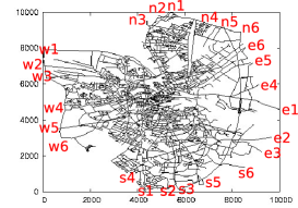
Figure 2: The OLB road network and its 24 entrances/exits.

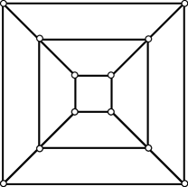
(a)	(b)

Figure 3: Examples of backbone networks: (a) grid-based with 10 roads, (b) ring-based with 16 roads.

5.1 Setup

Our experimental analysis involves both real and synthetic road networks. We use the real road networks of the following cities taken from OpenStreetMap: Oldeburg (OLB), Berlin (BER), Vienna (VIE) and Athens (ATH), containing $1,672$ roads and $2,383$ intersections, $15,246$ roads and $25,321$ intersections, $20,224$ roads and $27,563$ intersections, and $76,896$ roads and $108,156$ intersections, respectively. The weighted average degree of an intersection in these road networks is $2.09$, $2.15$, $2.17$ and $2.19$, respectively.

To study the scalability of our methodology we also generated synthetic road networks by populating the OLB road network. The idea is the following. In an attempt to capture the structure of a real network, a synthetic road network is defined as a set of neighborhoods connected to each other through a backbone road network. OLB is used to capture the internal road network of a neighborhood. Figure 2 pictures the 24 intersections used to enter/exit the internal road network of a neighborhood from/to the backbone.

Finally, to construct a backbone network we consider two different topologies. The grid-based topology of degree $\tau$ is constructed by $2\tau$ roads, $\tau^{2}$ intersections, and defines $(\tau-1)^{2}$ neighborhoods. On the other hand, a ring-based topology of degree $\tau$ is constructed by $4(\tau+1)$ roads, $4\tau$ intersections, and defines $4(\tau-1)+1$ neighborhoods. Figure 3(a) and (b) show an example of a grid-based and a ring-based backbone road network of degrees 5, and 3, respectively. The grid-based backbone consists of 10 roads connected through 25 intersections and defines 16 neighborhoods, while the ring-based backbone consists of 16 roads connected through 12 intersections and defines 9 neighborhoods.

To assess the performance of the routing methods, we measure their average response time and the average number of routes examined over $1,000$ queries. Finally, in case of the simplest near-fastest and the fastest near-simplest route problems, we test the methods varying $\epsilon$ inside $\{0.01,0.05,$ $0.1,0.2,0.3\}$.

5.2 Comparison of Routing Methods

Table 2: Real road networks: performance analysis for solving Problems 1 and 1.

	BSL		FS		SF
road	Response	Routes	Response	Routes	Response	Routes
network	time (sec)	examined	time (sec)	examined	time (sec)	examined
OLB	$68.7$	$121,236,000$	$0.003$	$2286.82$	$0.003$	$2418.35$
BER	$-$	$-$	$0.055$	$27226.3$	$0.040$	$27611.7$
VIE	$-$	$-$	$0.057$	$29301.8$	$0.042$	$29250.8$
ATH	$-$	$-$	$0.346$	$117,973$	$0.207$	$120,329$

The first set of experiments involves the OLB, BER, VIE, and ATH real road networks with the purpose of identifying the best method for each of the problems at hand.

Table 2 demonstrates the results for the fastest simplest and the simplest fastest route problems. We first observe that FS outperforms BSL by several orders of magnitude. In fact, we managed to execute BSL only on the smallest road network (OLB) due to its extremely high response time. This is expected as BSL needs to enumerate an enormous number of routes to identify the final answer. On the other hand, we observe that FS, SF identify the corresponding routes in less than half a second for all real networks.

Finally, we investigate which is the best method for the fastest near-simplest and the simplest near-fastest route problems. Note that for the purpose of this experiment we include two additional methods termed FNS-A^∗-WB and SNF-A^∗-WB. These algorithms follow the same principle as FNS-A^∗ and SNF-A^∗ respectively, without however invoking the AllFastestSimplest and AllSimplestFastest procedures (equivalently they assume $sfL[n]=sfC[n]=fsL[n]=fsC[n]=0$ for any node $n$). In addition, note that because of their high response time, we were able to execute FNS-DFS and SNF-DFS only on the smallest road network, OLB. Figure 4 clearly shows that FNS-A^∗ and SNF-A^∗ are the dominant methods for the problems at hand. In fact with the exception of the smallest road network, OLB, they outperform their competitors by at least one order of magnitude. The superiority of FNS-A^∗ (SNF-A^∗) over FNS-A^∗-WB (SNF-A^∗-WB) supports our decision to invoke the AllFastestSimplest and AllSimplestFastest procedures before the actual search takes place.

We also observe that as $\epsilon$ increases, the response time of the methods that solve simplest near-fastest route problem decreases. Specifically, the response time of SNF-A^∗-WB always decreases while the time of SNF-A^∗ first increases and after $\epsilon=0.1$ or $\epsilon=0.2$ it drops. Note that this trend is also followed by the average number of routes examined by the methods. The reason for is that the larger $\epsilon$ is, the more routes have acceptable length and thus need to be examined. At the same time, however, it is more likely to early identify a candidate answer, which can enhance the pruning mechanism and thus accelerate the query evaluation.

$\epsilon$	$\epsilon$	$\epsilon$	$\epsilon$
(a) OLB	(b) BER	(c) VIE	(d) ATH

Figure 4: Real road networks: performance analysis for solving Problems 1 and 1.

5.3 Scalability Tests

$\tau$	$\tau$	$\tau$	$\tau$
(a) grid-based	(b) grid-based	(c) ring-based	(d) ring-based

Figure 5: Synthetic road networks: scalability tests for $\epsilon=0.1$.

In the last set of experiments we study the scalability of the best methods identified in the previous section, i.e., FS, SF, FNS-A^∗ and SNF-A^∗. For this purpose, we generate synthetic road networks varying the degree of the topology $\tau$, and thus, the size of the road network. Particularly, for a grid-based backbone network $\tau$ takes values inside $\{2,3,4,5\}$, while for a ring-based backbone inside $\{1,2,3,4\}$. Figure 5 reports on the scalability tests. As expected, the response time of all methods increases when the degree of the topology increases. Even for the expensive fastest near-simplest and the simplest near-fastest route problems, our methods always identify the answer in less than half a second for $\epsilon=0.1$. Although we do not include figures for other values of $\epsilon$, our experiments show that this holds for every other combination of $\tau$ and $\epsilon$.

6 Conclusion

This paper dealt with finding routes that are as simple and as fast as possible. In particular, it studied the fastest simplest, simplest fastest, fastest near-simplest, and simplest near-fastest problems, and introduced solutions to thems. The proposed algorithms are shown to be efficient and practical in both real and synthetic datasets.

Acknowledgments. This research was partially supported by the German Research Foundation (DFG) through the Research Training Group METRIK, grant no.​ GRK 1324, and the European Commission through the project “SimpleFleet”, grant no.​ FP7-ICT-2011-SME-DCL-296423.

References

- [1] I. Abraham, D. Delling, A. V. Goldberg, and R. F. Werneck. A hub-based labeling algorithm for shortest paths in road networks. In Experimental Algorithms, pages 230–241. Springer, 2011.
- [2] R. Bauer and D. Delling. Sharc: Fast and robust unidirectional routing. Journal of Experimental Algorithmics (JEA), 14:4, 2009.
- [3] R. Bauer, D. Delling, P. Sanders, D. Schieferdecker, D. Schultes, and D. Wagner. Combining hierarchical and goal-directed speed-up techniques for dijkstra’s algorithm. Journal of Experimental Algorithmics (JEA), 15:2–3, 2010.
- [4] T. H. Byers and M. S. Waterman. Determining all optimal and near-optimal solutions when solving shortest path problems by dynamic programming. Operations Research, 32(6):1381–1384, 1984.
- [5] T. Caldwell. On finding minimum routes in a network with turn penalties. Communications of the ACM, 4(2):107–108, 1961.
- [6] D. Delling, A. V. Goldberg, A. Nowatzyk, and R. F. Werneck. Phast: Hardware-accelerated shortest path trees. Journal of Parallel and Distributed Computing, 2012.
- [7] E. W. Dijkstra. A note on two problems in connexion with graphs. Numerische mathematik, 1(1):269–271, 1959.
- [8] M. Duckham and L. Kulik. “simplest” paths: Automated route selection for navigation. In Conference On Spatial Information Theory (COSIT), pages 169–185, 2003.
- [9] R. Geisberger, P. Sanders, D. Schultes, and D. Delling. Contraction hierarchies: Faster and simpler hierarchical routing in road networks. In Experimental Algorithms, pages 319–333. Springer, 2008.
- [10] R. Geisberger and C. Vetter. Efficient routing in road networks with turn costs. In Experimental Algorithms, pages 100–111. Springer, 2011.
- [11] A. V. Goldberg and C. Harrelson. Computing the shortest path: A search meets graph theory. In Proceedings of the sixteenth annual ACM-SIAM symposium on Discrete algorithms, pages 156–165. Society for Industrial and Applied Mathematics, 2005.
- [12] R. J. Gutman. Reach-based routing: A new approach to shortest path algorithms optimized for road networks. In ALENEX/ANALC, pages 100–111, 2004.
- [13] B. Jiang and X. Liu. Computing the fewest-turn map directions based on the connectivity of natural roads. International Journal of Geographical Information Science, 25(7):1069–1082, 2011.
- [14] H.-P. Kriegel, M. Renz, and M. Schubert. Route skyline queries: A multi-preference path planning approach. In ICDE, pages 261–272, 2010.
- [15] W. Matthew Carlyle and R. Kevin Wood. Near-shortest and k-shortest simple paths. Networks, 46(2):98–109, 2005.
- [16] R. H. Möhring, H. Schilling, B. Schütz, D. Wagner, and T. Willhalm. Partitioning graphs to speedup dijkstra’s algorithm. Journal of Experimental Algorithmics (JEA), 11:2–8, 2007.
- [17] T. A. J. Nicholson. Finding the shortest route between two points in a network. The Computer Journal, 9(3):275–280, 1966.
- [18] A. Raith and M. Ehrgott. A comparison of solution strategies for biobjective shortest path problems. Computers & Operations Research, 36(4):1299–1331, 2009.
- [19] P. Sanders and D. Schultes. Highway hierarchies hasten exact shortest path queries. In Algorithms–Esa 2005, pages 568–579. Springer, 2005.
- [20] F. Schulz, D. Wagner, and C. Zaroliagis. Using multi-level graphs for timetable information in railway systems. In ALENEX, pages 43–59. Springer, 2002.
- [21] S. Winter. Modeling costs of turns in route planning. GeoInformatica, 6(4):345–361, 2002.