Anderson Localization Phenomenon in One-dimensional Elastic Systems

Abstract

The phenomenon of Anderson localization of waves in elastic systems is studied. We analyze this phenomenon in two different set of systems: disordered linear chains of harmonic oscillators and disordered rods which oscillate with torsional waves. The first set is analyzed numerically whereas the second one is studied both experimentally and theoretically. In particular, we discuss the localization properties of the waves as a function of the frequency. In doing that we have used the inverse participation ratio, which is related to the localization length. We find that the normal modes localize exponentially according to Anderson theory. In the elastic systems, the localization length decreases with frequency. This behavior is in contrast with what happens in analogous quantum mechanical systems, for which the localization length grows with energy. This difference is explained by means of the properties of the reflection coefficient of a single scatterer in each case.

I Introduction

The discovery of Anderson localization phenomenon in quantum mechanics gave origin to one of the most important subjects in condensed matter physics since it has a crucial effect on the transport properties of materials. As a matter of fact, the original work of Anderson Anderson is among the most cited papers of the twentieth century. The theory of Anderson localization Anderson ; KramerMacKinnon studies the alterations in the localization properties of the wave functions brought about by disorder in the system. It is well known that in a perfect periodic material the allowed energy levels form a band structure and the wave functions associated with the allowed energies are extended along the whole system. In this case, when an electric field is applied to the material and the energy of the electrons is such that there exist empty levels with energy close to the Fermi energy, the electrons can move throughout the material and an electrical current is produced. However, if the system has random imperfections, for example when there are strange atoms in an otherwise ideal chemical composition or when there is abnormal spacing between some atoms due to dislocations, the wave functions could be localized in some region of the system, therefore affecting the conductivity. In the particular case of one-dimensional infinite disordered systems, any amount of disorder produces localization in all the wave functions except for a set of states with zero measure. Thus, band theory and the theory of Anderson localization allow us to understand why some materials conduct electricity and why others do not.

Anderson localization has also been observed in many classical wave like phenomena: in optics dalichaouch ; Chabanov ; StorzerGrossAegerterMaret ; aegerter ; SchwartzBartalFishmanSegev ; lagini , elasticity HeMaynard ; HeMaynard2 ; Maynard ; HuStrybulevychPageSkipetrovVanTiggelen ; floresanderson , water waves lindelof and cold atomic gases garreau . When the systems are translational invariant, on the one hand, the elastic wave amplitudes are extended. One also finds a band spectrum of frequencies in this case. The wave amplitudes become localized in the disordered elastic systems, on the other hand, as is also true in solid state physics. However, in the elastic experiments one can go beyond what is obtained in quantum mechanics, since we can measure the wave amplitudes at each point. This allows us to understand the Anderson localization phenomenon in a deeper way. In this work we study this phenomenon in two different sets of elastic systems: the special linear harmonic oscillator chains described in Fig. 1 of Section II, and the disordered elastic rods defined in Fig. 4 of Section III. For the first set of systems we present numerical results while for the disordered rods this work has an experimental part and a theoretical one. To discuss the wave localization we calculate the inverse participation ratio. We also present a brief discussion of the mean free path $\ell_{m}$.

II Linear Harmonic Oscillator Chain

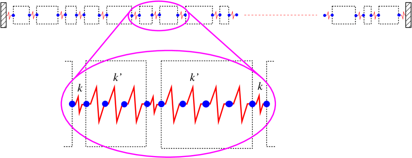
Figure 1: Disordered chain of harmonic oscillators. The zoom shows an amplification of two particular blocks with $N_{6}=3$ and $N_{7}=4$.

In this Section we analyze the first ensemble of elastic systems. Each member of the ensemble is a linear harmonic oscillator chain (LHOC), formed by $n$ identical point particles of mass $m$ coupled by $(n+1)$ springs, which in the general case have different strengths $k_{i}$. The two ends of each LHOC are fixed to walls with infinite mass. For homogeneous systems all the springs are equal to each other and the normal-mode frequencies can be obtained in closed form, as first done by Lagrange in 1788 Lagrange1788 . In the general case, the problem can be solved using the following well-known formalism.

The Lagrangian of the linear chain is

$$L=\dfrac{m}{2}\sum_{j=1}^{n}{\dot{\xi}_{j}^{2}-\frac{1}{2}\sum_{j=1}^{n+1}k_{j}\left(\xi_{j}-\xi_{j-1}\right)^{2}}$$ (1)

where $\xi_{j}(\textit{t})$ is the value of the coordinate of the j-th mass measured with respect its equilibrium value $\xi_{j}^{0}$; therefore $\xi_{n+1}=\xi_{0}=0,$ since they correspond to the infinite mass walls. The Lagrange equations take the form

$$m\ddot{\xi_{j}}=-k_{j}\xi_{j-1}+\left(k_{j}+k_{j+1}\right)\xi_{j}-k_{j+1}\xi_{j+1}.$$ (2)

When all the masses move with the normal mode of frequency $\omega_{I}$, that is, when $\xi_{j}\left(t\right)=\psi_{j}^{I}\exp\left(-i\omega_{I}t\right)$, where $\psi_{j}^{I}$ is the oscillation amplitude of mass j in the normal mode I, the following eigenvalue equation is obtained:

$$-k_{j}\psi_{j-1}^{I}+\left[\left(k_{j}+k_{j+1}\right)-m\omega_{I}^{2}\right]\psi_{j}^{I}-k_{j+1}\psi_{j+1}^{I}=0.$$ (3)

Solving Eq. (3) is equivalent to diagonalizing the matrix H with elements

$$H_{j,j-1} = -k_{j}$$

$$H_{j,j} = k_{j}+k_{j+1}$$ (4)

$$H_{j,j+1} = -k_{j+1}$$

and $H_{i,j}=0$ otherwise. In this process one obtains the normal-mode frequencies $\omega_{I}$ and the corresponding eigenvectors $\Psi_{I}=\left(\psi_{1}^{I},\psi_{2}^{I},\ldots,\psi_{n}^{I}\right)$.

Many different sets $\left\{k_{i}\right\}$ have been analyzed in the past Ashcroft . Here, we shall introduce a special set which behaves exactly as a vibrating rod with notches in compressional oscillations. We introduce a set of $\cal N$ blocks, each consisting of $N_{j}$ springs with strength $k^{\prime}$ and connected to their adjacent neighboring blocks by a spring of constant $k$. See Fig. 1. When $k^{\prime}>>k$ this system of blocks behave, for compressional oscillations, in a similar way as a vibrating elastic rod with notches; the soft springs play the role of the notches. Indeed, as will be published elsewhere, when all $N_{j}$ are identical to each other, the oscillator chain produces the band spectra we have found for a locally periodic rod with notches Moralesetal . Furthermore, we have also found that changing $N_{j}$ in such a way that

$$N_{j}=\left[{\frac{N}{1+j\gamma}}\right],$$ (5)

where $[x]$ means the largest integer not greater than $x$ and $\gamma$ is a real number, the Wannier-Stark ladder we encountered in Gutierrezetal is regained. Our oscillator chains are, as a consequence, useful to study disordered elastic systems and to learn how Anderson localization emerges.

We form the ensemble of LHOC’s in the following way: the family of numbers $\left\{N_{j}\right\}$, is a set of uncorrelated integer random numbers. The ensemble is defined with a uniform distribution in the interval $\left[N\left(1-\Delta\right),N\left(1+\Delta\right)\right]$. Here $N$ is the average of $N_{j}$ and $\Delta$ measures the disorder. In the results we show here, we used $N=70$ and $\Delta=2/7$. Each member of the ensemble has in general a different number of masses and springs.

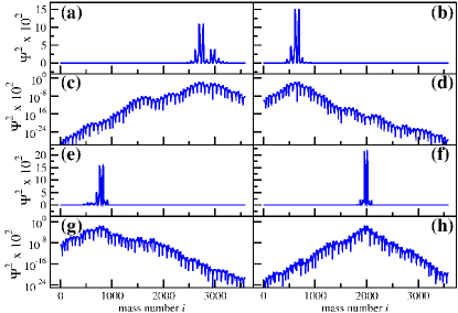
Figure 2: Square of wave amplitudes of four particular normal modes of a disordered linear chain.

We shall now present some results that show that Anderson localization arises. In Fig. 2, we show examples of $\left(\psi_{j}^{I}\right)^{2}$ for some particular normal-mode frequencies $\omega_{I}$ of a given member of the ensemble with ${\cal N}=50$. In Figs. 2(a), (b), (e), and (f), the values of $\left(\psi_{j}^{I}\right)^{2}$ are plotted in arbitrary units, whereas in Figs. 2(c), (d), (g), and (h), the same wave amplitudes are given but in a semi-log scale, respectively. The four values of I considered in this figure correspond to wave functions with 49, 54, 72, and 82 nodes, respectively. From these figures the localization of wave amplitudes is evident. Since the logarithmic plots are straight lines at both sides of the maxima, the wave amplitudes decrease exponentially on the average. One should mention that the wave functions with a number of nodes much less than $\cal N$ are not appreciably altered by the disorder since the wavelength is larger than the block size.

To discuss the localization properties of the ensemble of oscillator chains, we have calculated the inverse participation ratio (IPR). For a given eigenstate $\Psi^{I}$ the IPR is given by $\sum_{j}\left[\psi^{I}_{j}\right]^{4}$ and measures the number of sites that contribute significantly to the eigenfunction normalization. For states with an exponential decay, such as those given in Fig. 2, the IPR is directly connected with the localization length $\xi$ Fyodorov .

Figure 3: IPR^-1 as a function of $\omega$. The points are obtained from 50 different disordered chains with ${\cal N}=50$, $N=70$, $\Delta=2/7$ and $n\approx 3500$. The continuous line is a window average.

To calculate the average of the IPR we have considered an ensemble of systems like the one defined in Fig. 1. Then, we have calculated the IPR for all the eigenfunctions of the ensemble which have a normal-mode frequency in a certain eigenvalue interval. The points of Fig. 3 represent the values of the IPR^-1 of 50 different disordered chains. The continuous line shows the window average.

In order to construct the LHOC that simulates the behavior of a particular disordered rod we use the following procedure. Let us consider the rod of Fig. 4. If the length of the $j-th$ sub-rod is $d_{j}~{}$milimeters, then one constructs a block consisting of a linear chain with $[d_{j}]$ masses. Here $[d_{j}]$ means the largest integer not greater than $d_{j}$. These masses are joined by $[d_{j}]-1$ springs of strength $k^{\prime}$. Finally, as mentioned before, each block of masses is coupled with its neighboring blocks by means of springs of strength $k\ll k^{\prime}$. We have built, also with this procedure, the equivalent LHOC associated with the real rod studied in the laboratory. In Fig. 5 we show the values of the IPR^-1 as a function of frequency $\omega$ for this LHOC (full circles). We observe that the IPR^-1 decreases with frequency. The continuous line indicates a window average.

Measuring the time displacements of many particles subject to different springs is, however, a tough problem, which can become very cumbersome. Therefore, to perform experiments the oscillator chain will be replaced by an elastic rod with notches. We have already mentioned that the compressional modes for these rods behave identically to the special LHOC used here. However, we shall consider in the next section results for torsional vibrations for the two following reasons: On the one hand, one expects that compressional and torsional modes behave in a similar way since they obey the same equation; on the other hand, torsional waves are easier to measure with the experimental setup that we use. As we will see below, the IPR^-1 of Fig. 5 shows indeed similar results to those measured for the torsional modes of the rod given in Fig. 9.

Figure 4: Disordered rod which consists in a set of sub-rods of different length. The values of the parameters are $R_{L}=1.28\,{\rm cm}$, $\eta=R_{\varepsilon}/R_{L}=0.65$, $d=7.2\,{\rm cm}$, $\Delta=0.35$, $\varepsilon=1.016\,{\rm mm}$ and $N=50$.

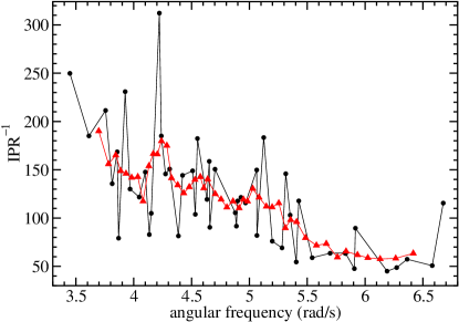
Figure 5: IPR^-1 as a function of $\omega$ for the special LHOC that simulates the real rod studied in the laboratory. The red triangles indicate a window average of 20 eigenvalues.

III Inhomogeneous Elastic Rod

We now study the torsional waves in rods with notches spaced at random along their axis. Each rod consists of a set of $\cal N$ coupled sub-rods with the same axis and radius $R_{L}$ and whose lengths are $d_{1},d_{2},...,d_{\cal N}$. The family $\{d_{i}\}$ is a set of $\cal N$ random uncorrelated lengths with a uniform distribution in the interval $[d(1-\Delta),d(1+\Delta)]$. Here $d$ is the average of $d_{i}$ and $\Delta$ measures the disorder. As shown in Fig. 4 the $\cal N$ sub-rods are joined by identical short cylinders of radius $R_{\varepsilon}=\eta R_{L}$ and length $\varepsilon\ll d_{i}$, $\forall i$. The parameter $\eta$, the coupling constant, satisfies the relation $0<\eta\leq 1$. For the experiment we have analyzed only one rod which was machined from a single aluminum piece. It should be mentioned that in the numerical simulations we have considered an ideal case of free conditions at the ends of the rod which is an approximation of the real configuration since the rod is supported by means of two thin threads. The frequency range we used in the experiment was 0-87 kHz and therefore

$$R_{L}=1.28{\rm\,cm}<\lambda_{\rm min}=\frac{c_{T}}{f_{\rm max}}=\frac{3140{\rm\,m/s}}{87000{\rm\,Hz}}=3.60{\rm\,cm},$$ (6)

which means that the cross section of the rod is not excited, so it behaves as a quasi one-dimensional system. The value of $c_{T}$ was measured by fitting the spectrum of the aluminium rod before machining the notches.

We have calculated numerically the set of eigenvalues $\{f_{i}\}$ and the corresponding eigenfunctions, using the Poincaré map method AvilaMendez-Sanchez . Then, the IPR as a function of frequency was obtained and an average of the localization length in some intervals of frequencies was calculated. The calculations were done with an effective value of the parameter $\eta$ as discussed in Refs. Moralesetal ; Moralesgutierrezflores .

To perform the measurements, the electromagnetic-acoustic transducer (EMAT) developed by us Moralesetal , was used. The EMAT consists of a permanent magnet and a coil, and can be used either to detect or excite the oscillations. The transducer operates through the interaction of eddy currents in the metallic rod with a permanent magnetic field. According to the relative position of the magnet and the coil, the EMAT can either excite or detect selectively compressional, torsional or flexural vibrations. Used as a detector, the EMAT measures acceleration. This transducer has the advantage of operating without mechanical contact with the rod. This is crucial to avoid perturbing the shape of the localized wave amplitudes. Both the detector and exciter are moved automatically along the rod axis by a computerized control system so the wave amplitudes can be measured easily (see Fig. 6).

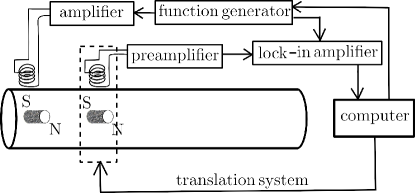
Figure 6: The experimental setup used to measure normal-mode amplitudes and frequencies of the rod of Fig. 4. Torsional waves are excited with the EMAT on the left side of this figure, whereas the detection is made with the EMAT placed on the translation system. In both EMAT’s the coil axis is perpendicular to the permanent magnet axis and these in turn are orthogonal to the rod axis.

Whenever the wave amplitude is measured, it is necessary to keep the system at resonance, so the wave generator must be as stable as possible. In order to achieve this, a Stanford Research Systems DS345 wave generator with an ovenized time base with stability $<0.01$ ppm was used in the experiment. This is enough when variations of the bar temperature are not important. In our case this condition was satisfied since the measurements were made in a very short time interval.

Before presenting the experimental and numerical results, we shall consider what we will call an independent rod model. This provides a qualitative argument to understand why all normal modes of a disordered rod are localized. The small sub-rods of length $d_{i}$ are independent of each other when $\eta\to 0$. The $i-{\rm th}$ sub-rod is excited when the driving force has a frequency $f$ equal to $f_{i}^{(q)}=pc_{T}/2d_{i}$, where $c_{T}$ is the speed of torsional waves and $p$ is an integer. The other sub-rods are, generally, not excited since $d_{j}$ is usually different from $d_{i}$. Hence, the amplitude of the vibration decreases and the wave amplitude is localized. Several experimental examples of this fact are shown in Fig. (7b), (7d) and (7f), where we have plotted the logarithm of the wave amplitude as a function of the coordinate $x$ along the rod. We observe that the envelope of the logarithm is a straight line at both sides of the maximum, which implies that the wave amplitude decreases as an exponential function. However, it could also happen that the length of some other sub-rod, say $d_{k}$, be almost equal to $d_{i}$. The amplitude of the vibration could then present two maxima. In Figs. (7a), (7c) and (7e) this case is apparent; we observe that they also decay exponentially. When the disorder is very small, that is $\Delta\ll 1$, the above argument implies that all the sub-rods can be excited with a driving frequency $f\sim pc_{T}/2d$ so the localization of the wave amplitude grows and it could even exceed the total length $L$ of the complete rod.

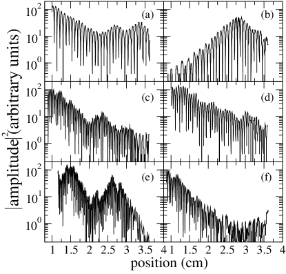
Figure 7: Measured localized wave amplitudes: (a) $f=18220$ Hz, (b) $f=18942$ Hz, (c) $f=34370$ Hz, (d) $f=25380$ Hz, (e)  $f=51553$ Hz, and (f) $f=35560$ Hz.

From this independent rod model we see that introducing disorder in the set $\{d_{i}\}$, whose first effect is to produce a disordered set of normal-mode frequencies, is a way to simulate a diagonal disorder in a quantum one-dimensional tight-binding hamiltonian where the coupling $\eta$ between first neighbors is equal to a constant. Therefore, the rods considered here are quasi one-dimensional disordered systems where the frequency plays the role of the energy in quantum mechanics. If all the sub-rods of radius $R_{L}$ have the same length, the vibrations of the rod are extended waves traveling in a periodic structure.

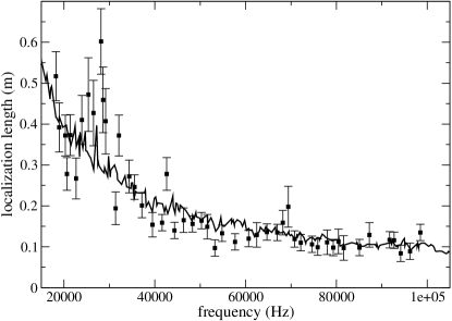
Figure 8: The localization length $\xi$ as a function of the frequency $f$. The dots correspond to the experimental measurements and the continuous line to the numerical average using an ensemble of 3000 rods.

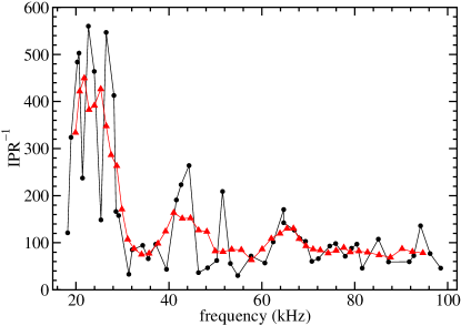
Figure 9: IPR^-1 as a function of the frequency $f$ for the rod studied in the laboratory. The triangles indicate a window average of 20 eigenvalues.

In the laboratory we have proceeded as follows. We have measured the values of the amplitude of each eigenfunction at a sufficiently large number of points of the rod and then, by using a least-squares fit, we have matched a function of the form $C\,\exp(-|x-x^{*}|/\xi)$ to their envelope; here $x^{*}$ is the position of the maximum of the amplitude. This provides us with the localization length $\xi$. Several eigenfunctions in each frequency interval were considered and the average of $\xi$ was evaluated. In most cases, we were able to measure the right-hand side of the wave amplitude only, because the exciter, placed at the left-hand side of the rod, produces a magnetic field in this zone that affects the measurements of the detector. With the purpose of adopting a systematic rule to define $\xi$ and its experimental error, we have taken into account only the side of the wave amplitude that decays exponentially towards the increasing values of $x$. The fit was always made taking into account only 10 points.

For some eigenmodes the fit could be done in two or three zones, so several values of $\xi$ were obtained. In these cases $\xi$ was defined as the average of these values. In Fig. 8 we show the experimental and numerical average values of $\xi$ as a function of the frequency $f$. A good agreement between the experiment and the numerical simulations is obtained. It is found that, in the elastic rods, the localization length $\xi$ of the normal modes decreases with the frequency. This is corroborated obtaining the participation ratio for the experimental rod; the IPR^-1 is shown in Fig. 9.

One should note that in the quantum mechanical analog, $\xi$ grows with the energy eigenvalue. This difference is not surprising if one analyzes the behavior of the individual scatterers that constitute the system in each case: a notch for the rod and a potential barrier for the quantum case. In particular, when one calculates the reflection coefficient $|r|^{2}$ as a function of the eigenvalue for the case of a notch one obtains:

$$|r|^{2}_{\rm classical}={4{\rm sen}^{2}(Q\varepsilon)\over\Big{(}{\eta^{4}-1\over\eta^{4}+1}-{\eta^{4}+1\over\eta^{4}-1}\Big{)}^{2}+4{\rm sen}^{2}(Q\varepsilon)},$$ (7)

whereas for the case of a quantum particle of mass $m$ in the presence of a rectangular barrier of height $U_{0}$ and width $\varepsilon$ one gets

$$|r|^{2}_{\rm quantum}={4{\rm sen}^{2}(q\varepsilon)\over\Big{(}{\tilde{\eta}^{4}-1\over\tilde{\eta}^{4}+1}-{\tilde{\eta}^{4}+1\over\tilde{\eta}^{4}-1}\Big{)}^{2}+4{\rm sen}^{2}(q\varepsilon)},$$ (8)

where $Q={2\pi f\over c_{T}}$, $q=\sqrt{{2m\over{\hbar}^{2}}(E-U_{0})}$, $\tilde{\eta}=\big{(}{E-U_{0}\over E}\big{)}^{1/8}$, and $\hbar$ is Planck’s constant divided by $2\pi$. In Fig. 10 we show a plot of $|r|^{2}_{\rm classical}$ as a function of $Q\varepsilon$. We can see that this is an increasing function of the eigenvalue in the range of frequencies we use, whereas in the quantum case it decreases with the energy. The crucial difference between the two cases is that in the elastic case $\eta$ is a constant determined by the geometry of the system, whereas in the quantum case $\tilde{\eta}$ is an increasing function of the energy. For these simple scatterers, we have also calculated the mean free path $\ell_{m}$ defined as $\ell_{m}\equiv\big{(}|r|^{2}/\Delta x\big{)}^{-1}$, where $|r|^{2}/\Delta x$ is the reflection coefficient per unit length. In our case we have taken $\Delta x=\varepsilon$. As a consequence of the previous discussion, the behavior of $\ell_{m}$ in the classical system we have considered is opposite to that in the quantum case. In particular, the classical $\ell_{m}$ is a decreasing function of the frequency whereas for the quantum case it is an increasing function of the energy.

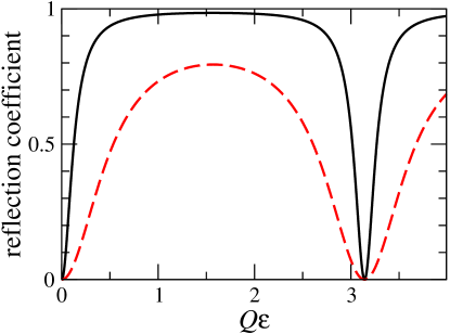
Figure 10: Reflection coefficient $|r|^{2}_{\rm classical}$ as a function of $Q\varepsilon$ for torsional waves through a notch. The continuous and dashed lines correspond to $\eta=0.5$ and $\eta=0.7$, respectively.

Note that in the classical case a reflection coefficient that increases with frequency indicates that the smaller the wavelength is, the more noticeable the defects, i.e., the notches, are. Therefore the defects tend to decrease the transmission when the wave length also decreases. In the quantum case one has a reflection coefficient that decreases with energy which indicates that the greater the wavelength is, the defects, i.e., the potential barriers, are less important. This fundamental difference between the quantum model and the classical system reflects the incapacity to simulate quantum potentials using rods with notches. Consequently, it is expected that in our experiments the dependence of the localization length as a function of frequency be opposite to that observed in the quantum case. Nevertheless, the Anderson localization phenomenon appears in both situations.

We now return to the discussion of systems with a large number of scatterers. Since the waves show an exponential decrease, it is expected that the square of the transmission coefficient $|t|^{2}=1-|r|^{2}$ shows an exponential decrease of the form

$$|t|^{2}=\exp\Big{(}-{x\over{\ell}^{\prime}_{m}}\Big{)},$$ (9)

where $\ell^{\prime}_{m}$ is a constant which, as is easy to see, is equal to the mean free path $\ell_{m}$. In fact, if we evaluate the above expression for $x=\Delta x\ll\ell^{\prime}_{m}$ we have

$$|t|^{2}=1-|r|^{2}=\exp\Big{(}-{\Delta x\over{\ell}^{\prime}_{m}}\Big{)}=1-{\Delta x\over\ell^{\prime}_{m}}$$ (10)

which implies that $\ell_{m}=\ell^{\prime}_{m}$.

IV Conclusions

In the present work two different sets of elastic disordered structures were analyzed. We have presented, both numerically and experimentally, evidence of the Anderson localization. The localization length of the normal modes as a function of frequency was measured on elastic rods by means of the wave amplitude as well as by the inverse participation ratio, and not by means of the transmittance. A good agreement between the numerical simulations and the experimental values was obtained. We have found that the localization length and the participation ratio decrease with the frequency, which is opposite to the quantum mechanical case.

V acknowledgements

This work is supported by DGAPA-UNAM under project IN113011. RAMS was supported by DGAPA-UNAM under project IN111311 and by CONACYT under project 79613. GM was supported by DGAPA UNAM project IN-117712-3. We are indebted to Pierric Mora for his help in the measurements.

References

- (1) P. W. Anderson, Phys. Rev. 109, 1492 (1958).
- (2) B. Kramer and A. MacKinnon, Rep. Prog. Phys. 56, 1469 (1993).
- (3) R. Dalichaouch, J. P. Armstrong, S. Schultz, P.M. Platzman, and S. L. McCall, Nature 354, 53 (1991).
- (4) A. A. Chabanov, M. Stoytchev, and A.Z. Genack, Nature 404, 850 (2000).
- (5) M. Störzer, P. Gross, C. M. Aegerter and G. Maret, Phys. Rev. Lett. 96, 063904 (2006)
- (6) C. M. Aegerter, M Störzer, and G. Maret, Europhys Lett. 75, 562 (2006).
- (7) T. Schwartz, G. Bartal, S. Fishman and M. Segev, Nature 446, 52 (2007).
- (8) Y. Lahini, A. Avidan, F. Pozzi, M. Sorel, R. Morandotti, D. N., Christodoulides, and Y. Silberberg, Phys. Rev. Lett. 100, 013906 (2008).
- (9) S. He and J. D. Maynard, Phys. Rev. Lett. 57, 3171 (1986).
- (10) S. He and J. D. Maynard, Phys. Rev. Lett. 62, 1888 (1989).
- (11) J. D. Maynard, Rev. Mod. Phys. 73, 401 (2001).
- (12) H. Hu, A. Strybulevych, J. H. Page, S. E. Skipetrov and B. A. van Tiggelen, Nature Phys. 4, 945 (2008)
- (13) J. Flores, L. Gutiérrez, R. A. Méndez-Sánchez, G. Monsivais, P. Mora and A. Morales, EPL 101, 67002 (2013).
- (14) P. E. Lindelof, J. Norregaard, and Hanberg, Phys. Scr. T 14, 17 (1986).
- (15) G. Lemarie, H. Lignier, D. Delande, P. Szriftgiser, and J. C. Garreau, Phys. Rev. Lett. 105 (2010) 090601.
- (16) J. L. Lagrange, Mecanique Analytique, Seconde Partie.-La dynamique, (Paris, 1788) Sect. VI p. 339.
- (17) N. W. Ashcroft and N. D. Mermin, Solid State Physics, (Holt, Rinehart and Winston, New York 1976).
- (18) A. Morales, J. Flores, L. Gutiérrez, and R. A. Méndez-Sánchez, J. Acoust. Soc. of Am. 112, 1961 (2002).
- (19) A. Díaz-de-Anda, A. Pimentel, J. Flores, A. Morales, L. Gutierrez, and R. A. Méndez-Sánchez, J. Acoust. Soc. Am. 117, 2814-2819 (2005).
- (20) L. Gutiérrez, A. Díaz-de-Anda, J. Flores, R. A. Méndez-Sánchez, G. Monsivais, and A. Morales, Phys. Rev. Lett. 97, 114301 (2006).
- (21) Y. V. Fyodorov and A. D. Mirlin, Phys. Rev. Lett. 71, 412 (1993).
- (22) M. A. Ávila and R. A. Méndez-Sánchez, Physica E 30, 174 (2005).
- (23) A. Morales, L. Gutiérrez and J. Flores, Am. J. Phys. 69, 517 (2001).