A Metric-learning based framework for Support Vector Machines and Multiple Kernel Learning

Abstract

Most metric learning algorithms, as well as Fisher’s Discriminant Analysis (FDA), optimize some cost function of different measures of within-and between-class distances. On the other hand, Support Vector Machines(SVMs) and several Multiple Kernel Learning (MKL) algorithms are based on the SVM large margin theory. Recently, SVMs have been analyzed from a metric learning perspective, and formulated as a Mahalanobis metric learning problem. This new perspective allows us to combine ideas from both SVM and metric learning, and to develop new algorithms that build on the strengths of each. Inspired by the metric learning interpretation of SVM, we develop here a new metric-learning based SVM framework in which we incorporate metric learning concepts within SVM. We extend the optimization problem of SVM to include some measure of the within-class distance and along the way we develop a new within-class distance measure which is appropriate for SVM. In addition, we adopt the same approach for MKL and show that it can be also formulated as a Mahalanobis metric learning problem. Our end result is a number of SVM/MKL algorithms that incorporate metric learning concepts. We experiment with them on a set of benchmark datasets and observe important predictive performance improvements.

I Introduction

Support Vector Machines [5] have been an active research area for more than two decades. They have been widely used not only because of their excellent predictive performance but also because their generalization ability is supported by solid generalization error bounds defined over the radius-margin ratio. Mahalanobis metric learning has started attracting significant attention rather recently [16, 18, 22, 20, 3, 23, 13, 12]. However, relying mostly on intuition, it still lacks theoretical support. Very recently SVM has been reformulated in the metric learning context and has been shown to be equivalent to a Mahalanobis metric learning problem [9]. This new interpretation of SVM brings the worlds of SVM and metric learning together into a single unified view. This allows us to exploit the advantages of each one to develop for example hybrid algorithms or to derive theoretical error bounds for metric learning problems exploiting the SVM error bounds.

In this paper we build on the ideas presented in [9] to develop a novel metric-learning-based SVM framework and equip SVM with a metric learning bias. More precisely we will define new SVM optimization problems that will make use of both the between-and within-class distances. Under the metric learning view of SVM, the margin plays the role of the between-class distance. However, SVM ignores the within-class distance. In the metric-learning-based SVM framework that we present here, we maximize the SVM margin and minimize some measure of the within-class distance. We can use different measures of the within-class distance with SVM and we will define a new such measure that is more appropriate for SVM. We will give a new SVM algorithm that optimizes both the margin and the new within-class distance measure that we define. The resulting optimization problem is convex and can be directly kernelized. Moreover we will follow the same approach with MKL and show that it, also, can be formulated as a Mahalanobis metric learning problem. As a result we develop a novel family of MKL methods that incorporate the metric learning bias. We experiment with the developed algorithms on a number of benchmark datasets and saw that the incorporation of the within-class distance measures in the SVM learning problem brings significant performance improvements.

Finally, we give a unified view of SVM, metric-learning-based SVM, metric learning algorithms and Fisher Discriminant Analysis (FDA) using the concepts of between-class and within-class distances. This view provides new insights to the existing algorithms and unveils some unexpected relations.

The rest of the paper is organized as follows. In the next section we briefly describe the basic concepts of SVM, FDA and Mahalanobis metric learning. In section III we summarize the metric learning view of SVM. In section IV we propose the metric-learning-based SVM framework which relies on the use of the between-class and within-class distance measures. In section V we provide a common view of SVM, metric-learning based SVM, FDA and metric learning algorithms. In Section 5 we employ the metric learning perspective in the context of MKL and develop the metric-learning-based MKL framework. We report experimental results in section VII and conclude with section VIII.

II Preliminary

Consider a binary classification problem in which we are given a set of $n$ learning instances $S=\{({\mathbf{x}}_{1},y_{1}),...,({\mathbf{x}}_{n},y_{n})\},{\mathbf{x}}_{i}\in{\mathcal{R}}^{d}$, where $y_{i}$ is the class label of the ${\mathbf{x}}_{i}$ instance and $y_{i}\in\{+1,-1\}$. Let $\mathcal{D}_{i}=\{{\mathbf{x}}_{j}|y_{j}=C_{i}\}$ be the samples of class $C_{i}$.

II-A Support Vector Machines and MKL

SVMs learn a hyperplane $H_{\mathbf{w}}:{\mathbf{w}}^{T}{\mathbf{x}}+b=0$ which maximizes the margin between the two classes. The SVM margin is defined informally as the distance of the nearest instances from $H_{\mathbf{w}}$ [5]. The SVM optimization problem is:

$$\min_{\mathbf{w},\boldsymbol{\xi},b} \|{\mathbf{w}}\|^{2}_{2}+C\sum_{i=1}^{l}\xi_{i}$$ (1)

$$s.t. y_{i}({\mathbf{w}}^{T}{\mathbf{x}}_{i}+b)\geq 1-\xi_{i},\forall i$$

The performance of SVM strongly depends on the choice of kernel. MKL addresses that problem by selecting or learning the appropriate kernel(s) for a given problem [16, 6, 18, 20, 4, 22, 1]. Given a set of basis kernel functions, $\boldsymbol{Z}=\{K_{k}({\mathbf{x}},{\mathbf{x}}^{\prime})|k:=1\dots m\}$, MKL learns a kernel combination, usually convex, so that some cost function, e.g margin, kernel alignment, is optimized. The cost function that is most often used in MKL is the margin-based objective function of SVM [20, 4, 22, 1, 16, 15]. We denote by $MKL_{\gamma}$ the MKL method which learns linear kernel combinations and uses as its cost function that of standard SVM, i.e. it finds a linear kernel combination that maximizes the margin. Its optimization problem is:

$$\min_{{\mathbf{w}},b,\boldsymbol{\xi},\boldsymbol{\mu}} \frac{1}{2}\sum_{k}^{m}\langle{\mathbf{w}}_{k},{\mathbf{w}}_{k}\rangle+\frac{C}{2}\sum_{i=1}^{l}\xi_{i}^{2}$$ (2)

$$s.t. y_{i}(\sum_{k}^{m}\langle{\mathbf{w}}_{k},\sqrt{\mu_{k}}\mathbf{\Phi}_{k}({\mathbf{x}}_{i})\rangle+b)\geq 1-\xi_{i},\forall i$$

$$\|\boldsymbol{\mu}\|_{p}=1,\mu_{k}\geq 0,\forall k$$

II-B Mahalanobis metric learning

The squared Mahalanobis distance between two instances ${\mathbf{x}}_{i}$ and ${\mathbf{x}}_{j}$ is: $d_{\mathbf{M}}^{2}({\mathbf{x}}_{i},{\mathbf{x}}_{j})=({\mathbf{x}}_{i}-{\mathbf{x}}_{j})^{T}\mathbf{M}({\mathbf{x}}_{i}-{\mathbf{x}}_{j})$ where $\mathbf{M}$ is a positive semi-definite matrix, $\mathbf{M}\succeq 0$. Learning a Mahalanobis metric parametrized by $\mathbf{M}$ ($\mathbf{M}\succeq 0$) is equivalent to learning a linear transformation $\mathbf{A}$ where $\mathbf{A}^{T}\mathbf{A}=\mathbf{M}$.

Typical metric learning methods try to bring instances of the same class close while pushing instances of different classes far away. They do so by optimizing a cost function of the Mahalanobis distance, while globally or locally satisfying some constraints on the pairwise distances. This is equivalent to minimize some measure of the within-class distances while maximizing the between-class distances [9].

A typical Mahalanobis metric learning optimization problem has the following form:

$$\min_{\mathbf{M}\succeq 0} F(\{d_{\mathbf{M}}^{2}({\mathbf{x}}_{i},{\mathbf{x}}_{j})|{\mathbf{x}_{i},\mathbf{x}_{j}\in S}\}) s.t.\,{\mathcal{C}onstraints}$$ (3)

$$\Leftrightarrow$$

$$\min_{\mathbf{A}} F(\{d_{\mathbf{A}}^{2}({\mathbf{x}}_{i},{\mathbf{x}}_{j})|{\mathbf{x}_{i},\mathbf{x}_{j}\in S}\}) s.t.\,{\mathcal{C}onstraints}$$

where $F$ and $\mathcal{C}onstraints$ are the cost function and the constraints respectively, parametrized either by $\mathbf{M}$ or $\mathbf{A}$. The constraints can be local, i.e applied to instance pairs that are in the same neighborhood, or global, i.e applied for all instance pairs. They usually have the following form [24, 12, 7, 23]:

$$d_{\mathbf{M}}^{2}({\mathbf{x}}_{i},{\mathbf{x}}_{j}) \leq f_{1},\,if\,y_{i}=y_{j}$$ (4)

$$d_{\mathbf{M}}^{2}({\mathbf{x}}_{i},{\mathbf{x}}_{j}) \geq f_{2},\,if\,y_{i}\neq y_{j}$$

for some constants $f_{1},f_{2}$. These constraints reflect the primal bias of most metric learning algorithms, maximizing the between-class distance and minimizing the within-class distance, or in other words, instances of the same class should have small distances while those of different classes should have large distances. If we take two simple measures of the within and between-class distances such as the sum of the pairwise distances of the same-class instances and the sum of the pairwise distances of the different-class instances respectively, the pairwise constraints in (4) will ensure that our between-class distance, denoted by $d_{B}$, is bigger than $f_{2}\times t_{1}$, and our within-class distance, denoted by $d_{W}$, is smaller than $f_{1}\times t_{2}$, where $t_{1},t_{2}$ are the numbers of instance pairs of the same and different class respectively over which we impose the constrains..

II-C Fisher Discriminant Analysis

FDA, although usually not considered a metric learning method, it also learns linear projections in the same manner as metric learning methods. It uses a similar learning bias as metric learning algorithms: the samples are well separated if their between-class distance is large and their within-class distance is small. These quantities are defined as follows [17]: let the sample mean of class $C_{i}$ be $\boldsymbol{m}_{i}=\frac{1}{n_{i}}\sum_{{\mathbf{x}}\in\mathcal{D}_{i}}{\mathbf{x}}$, then the within-class distance (or within-class scatter) of two classes $C_{1},C_{2},$ is defined as $s_{w}=\sum_{i=1,2}\sum_{{\mathbf{x}}\in\mathcal{D}_{i}}\|{\mathbf{x}}-\boldsymbol{m}_{i}\|^{2}$, and the between-class distance (or between-class scatter) is defined as the squared distance between the means of the two classes, $s_{b}=\|\boldsymbol{m}_{i}-\boldsymbol{m}_{j}\|^{2}$. In the case of two-class problems FDA seeks for a projection line with a direction vector ${\mathbf{w}}$ which optimizes the ratio of the between-class over the within-class distances in the projected space, its cost function is:

$$\max_{{\mathbf{w}}}\,\,\,\,J({\mathbf{w}}) = \frac{s_{b,{\mathbf{w}}}}{s_{w,{\mathbf{w}}}}=\frac{({\mathbf{w}}^{T}(\boldsymbol{m}_{1}-\boldsymbol{m}_{2}))^{2}}{\sum_{i}\sum_{{\mathbf{x}}\in\mathcal{D}_{i}}({\mathbf{w}}^{T}({\mathbf{x}}-\boldsymbol{m}_{i}))^{2}}$$ (5)

$$= \frac{{\mathbf{w}}^{T}\mathbf{S}_{\mathbf{W}}{\mathbf{w}}}{{\mathbf{w}}^{T}\mathbf{S}_{\mathbf{B}}{\mathbf{w}}}$$

where $\mathbf{S}_{\mathbf{W}}=\sum_{i=1,2}\sum_{{\mathbf{x}}\in\mathcal{D}_{i}}({\mathbf{x}}-\boldsymbol{m}_{i})({\mathbf{x}}-\boldsymbol{m}_{i})^{T}$ and $\mathbf{S}_{\mathbf{B}}=(\boldsymbol{m}_{1}-\boldsymbol{m}_{2})(\boldsymbol{m}_{1}-\boldsymbol{m}_{2})^{T}$ are the within-class and between-class scatter matrices, respectively. Another measure often used in the different variants of FDA is the total scatter matrix, $\mathbf{S}_{\mathbf{T}}=\mathbf{S}_{\mathbf{W}}+\mathbf{S}_{\mathbf{B}}$, i.e a multiply of the covariance matrix which quantifies the total data spread.

III Related work

Do et al [9] recently show SVM can be formulated as a Mahalanobis metric learning problem in which the transformation matrix is diagonal $\mathbf{W}$, $diag(\mathbf{W})={\mathbf{w}}=(w_{1},\dots,w_{d})^{T},\|\mathbf{w}\|_{2}=1$. In the metric learning jargon SVM learns a diagonal linear transformation $\mathbf{W}$ and a translation $b$ which maximize the margin and place the two classes symmetrically in the two different sides of the hyperplane $H_{\boldsymbol{1}}:\boldsymbol{1}^{T}{\mathbf{x}}=0$. In the standard view of SVM, the space is fixed and the hyperplane is moved around to achieve the optimal margin. In the metric view of SVM, the hyperplane is fixed to $H_{\boldsymbol{1}}$ and the space is scaled, $\mathbf{W}$, and then translated, $b$, so that the instances are placed optimally around $H_{\mathbf{1}}$ [9].

[9] proposed a measure of the within-class distance for SVM. This measure is inspired by the relation, developed in that paper, between SVM and LMNN—Large Margin Nearest Neighbor [23]—a popular metric learning algorithm. It is defined as the sum of the distances of the instances from the margin hyperplane and for the class $C_{i}$, it is given by: $d^{i}_{W_{1}}=\sum_{{\mathbf{x}}\in C_{i}}(|d({\mathbf{x}},H_{w})|-\gamma)$. The authors then proposed an SVM variant, called $\epsilon$-SVM, which optimizes the margin and the above within-class distance measure, essentially combining both the SVM and the LMNN learning biases. As we will see below $\epsilon$-SVM turns out to be a special case of the $SVM_{m}$ which we will describe in section IV-B1. The optimization problem of $\epsilon$-SVM is:

$$\min_{{\mathbf{w}},b} \mathbf{w}^{T}\mathbf{w}+\lambda\sum_{i}max(0,y_{i}(\mathbf{w}^{T}\mathbf{x}_{i}+b)-1)$$ (6)

$$+C\sum_{i}max(0,1-y_{i}(\mathbf{w}^{T}\mathbf{x}_{i}+b))$$

which is equivalent to:

$$\min_{{\mathbf{w}},b,\boldsymbol{\xi},\boldsymbol{\eta}} {\mathbf{w}}^{T}{\mathbf{w}}+C_{1}\sum_{i}^{n}{\xi_{i}}+C_{2}\sum_{i}^{n}{\eta_{i}}$$ (7)

$$s.t. 1-\xi_{i}\leq y_{i}({\mathbf{w}}^{T}{\mathbf{x}}_{i}+b)\leq 1+\eta_{i}$$

$$\xi_{i}\geq 0,\eta_{i}\geq 0,\forall i$$

where $\eta_{i}$ is the distance of the $i$th instance from its margin hyperplane, and $\xi_{i}$ are the SVM slack variables which allow for the soft margin. This problem is convex and can be kernelized directly as a standard SVM.

[21] proposed to maximize the margin and to constrain the outputs of SVM, their optimization problem thus optimizes the margin and some measure of the data spread. This approach also falls within our general metric-learning-based SVM framework that we will present right away.

IV A metric-learning-based SVM framework

Since SVM can be seen as a metric learning algorithm, we can interpret it in terms of the within- and between-class distances, as is done with typical metric learning algorithms using (3), (4). The SVM margin can be seen as a measure of the between-class distance. Unlike FDA where the between-class distance is defined via the distance of the class means, in SVMs, it is defined as the minimum distance of different-class instances from the hyperplane, i.e. twice the SVM margin. Unlike other metric learning algorithms, where the between-class distance takes into account all pairs of instances of different classes, the SVM between-class distance only focuses on pairs of instances of different classes which lie on the margin (in [9], the SVM margin is reformulated as: $\min_{i,j,y_{i}\neq y_{j}}(\mathbf{x}_{i}-\mathbf{x}_{j})^{T}\mathbf{w}^{T}\mathbf{w}(\mathbf{x}_{i}-\mathbf{x}_{j})$). In other words, SVM between-class distance, i.e the margin, is a simple example of (4).

Similar to most metric learning algorithms, SVM maximizes the between-class distance; however, unlike them, it ignores the within-class distance. In other words, instances of different classes are pushed far away by the margin, but there is no constraint on instances of the same class.

Interpreting SVM as a metric learning problem allows us to fully equip it with the metric learning primal bias, i.e to maximize some between-class distance measure and minimize some within-class distance measure. We propose a learning framework in which in addition to the standard SVM margin maximization, we also minimize some measure of the within-class distance. We will call the resulting learning algorithms metric-learning-based SVM. In the next sections we will give different general functions of the within and between class distances which can be the target of optimization. We will then propose SVM specific within-class distance measures, and finally formulated the full learning problem which now will also include some measure of the within class distance.

IV-A Within- and between-class distances cost functions

There are several ways to maximize the between-class distances $d_{B}$ while minimizing the within-class distances $d_{W}$. Bellow we give some simple and widely used cost functions that include these two terms:

$$\max F_{1}=\frac{d_{B}}{d_{W}}$$ (8)

$$\max F_{2}=d_{B}+\lambda\frac{1}{d_{W}}$$ (9)

$$\max F_{3}=d_{B}-\lambda d_{W}$$ (10)

$$\min F_{4}=\frac{1}{d_{B}}+\lambda d_{W}$$ (11)

Depending on the exact measures of the within- and between-class distances, these cost functions will lead to convex or non-convex optimization problems. An example of the first cost function $F_{1}$ of (8) is FDA (5) where the resulting optimization problem is convex and easy to solve. $F_{1}$ places equal importance on the between- and within-class distances. On the other hand $F_{2},F_{3}$, and $F_{4}$ allow us to better control their trade-off through the introduction of an additional hyperparameter $\lambda$. Within our metric-learning-based SVM framework, $d_{B}$ will denote the margin, and $d_{W}$ will denote some measure of the within-class distance

IV-B Metric-learning based SVM

In this section we start by presenting a new measure of the within-class distance $d_{W}$ which is appropriate for SVM. We will then use this measure to define one instantiation of our metric-learning-based SVM framework. In addition, we discuss a number of other within-class distance measures which can be used to define other instantiations of our framework.

IV-B1 A bandwidth-based within-class distance measure

One way to control the within-class distance is by forcing the learning instances to stay close to their class margin hyperplane, confining them within a band defined by their margin hyperplane and a hyperplane parallel to it. The width of this band can be seen as a measure of the within-class distance. This bandwidth is equal to the maximum distance of the instances to their class margin given by $d^{i}_{W_{2}}=\max_{{\mathbf{x}}\in C_{i}}|d({\mathbf{x}},H_{{\mathbf{w}}})|-\gamma$. To avoid the effect of outlier instances we add slack variables that allow some of them to lie outside the band.

We introduce now a new SVM variant, which optimizes both the margin and the measure of the within-class distance described above. Its cost function trades-off the margin maximization and the bandwidth minimization. Let $d^{i}_{W_{2}}=\epsilon_{i}\gamma$, $\epsilon_{i}$ states how many times is the bandwidth of the $C_{i}$ class larger than the margin. To simplify the optimization problem we use the same $\epsilon=\epsilon_{1}=\epsilon_{2}$ for both bandwidths. Using the cost function given in equation (10), we get the following optimization problem:

$$\max_{{\mathbf{w}},b,\gamma,\epsilon} \gamma-\lambda\epsilon\gamma$$ (12)

$$s.t. \frac{y_{i}({\mathbf{w}}^{T}{\mathbf{x}}_{i}+b)}{\|\mathbf{w}\|_{2}}\geq\gamma,\forall i$$

$$\frac{y_{i}({\mathbf{w}}^{T}{\mathbf{x}}_{i}+b)}{\|\mathbf{w}\|_{2}}\leq\gamma+\epsilon\gamma,\forall i$$

$$\gamma\|{\mathbf{w}}\|_{2}=1,\,\,\epsilon\geq 0$$

$$\Leftrightarrow\max_{{\mathbf{w}},b,\epsilon} (1-\lambda\epsilon)/\|{\mathbf{w}}\|_{2}^{2}$$ (13)

$$s.t. y_{i}({\mathbf{w}}^{T}{\mathbf{x}}_{i}+b)\geq 1$$

$$y_{i}({\mathbf{w}}^{T}{\mathbf{x}}_{i}+b)\leq 1+\epsilon,\forall i,\,\,\epsilon\geq 0$$

Problem (13) is not convex, however, it can be easily kernelized as standard SVM. If we fix $\epsilon$ then it becomes convex. Fixing $\epsilon$ is equivalent to fixing a specific value for the margin-bandwidth ratio and then maximizing the margin; this is described by the following optimization problem:

$$\min_{{\mathbf{w}},b,\boldsymbol{\xi},\boldsymbol{\eta}} \|{\mathbf{w}}\|^{2}_{2}+C_{1}\sum\xi_{i}+C_{2}\sum\eta_{i}$$ (14)

$$s.t. y_{i}({\mathbf{w}}^{T}{\mathbf{x}}_{i}+b)\geq 1-\xi_{i}$$

$$y_{i}({\mathbf{w}}^{T}{\mathbf{x}}_{i}+b)\leq 1+\epsilon+\eta_{i},\forall i$$

$$\boldsymbol{\xi},\boldsymbol{\eta}\geq 0$$

where $\boldsymbol{\xi}$ and $\boldsymbol{\eta}$ are the slack variables that allow for the margin and bandwidth violations, the latter is needed to alleviate the effects of outlier instances. Intuitively the hyperparameter $C_{2}$, which controls the bandwidth slack variable, should be bigger than $C_{1}$ which controls the margin slack variable, since we can tolerate more instances outside the band than inside the margin.

Problem (14) is convex, quadratic and can be solved similarly to standard SVM. We will call it $SVM_{m}$. Its dual form is:

$$\max_{\boldsymbol{\alpha},\boldsymbol{\beta}} \sum_{i}^{n}(\alpha_{i}-(1+\epsilon)\beta_{i})$$

$$-\frac{1}{2}\sum_{ij}^{n}(\alpha_{i}-\beta_{i})(\alpha_{j}-\beta_{j})y_{i}y_{j}{\mathbf{x}}^{T}_{i}{\mathbf{x}}_{j}$$

$$s.t. \sum_{i}(\alpha_{i}-\beta_{i})y_{i}=0$$

$$0\leq\alpha_{i}\leq C_{1},\forall i$$

$$0\leq\beta_{i}\leq C_{2},\forall i$$

It can be also kernelized directly as SVM, as the term ${\mathbf{x}}_{i}^{T}\mathbf{x}_{j}$ that appears in the dual form (IV-B1) can be replaced by a kernel function.

Using the $F_{4}$ cost function (11) we get the following non-convex optimization problem which also “maximizes the margin while keeping the bandwidth $d^{i}_{W_{1}}$ small”:

$$\min_{{\mathbf{w}},b,\gamma,\epsilon} \frac{1}{\gamma^{2}}+\lambda\epsilon^{2}\gamma^{2}$$ (16)

$$s.t. \frac{y_{i}({\mathbf{w}}^{T}{\mathbf{x}}_{i}+b)}{\|\mathbf{w}\|_{2}}\geq\gamma$$

$$\frac{y_{i}({\mathbf{w}}^{T}{\mathbf{x}}_{i}+b)}{\|\mathbf{w}\|_{2}}\leq\gamma+\epsilon\gamma,\forall i$$

$$\gamma\|{\mathbf{w}}\|_{2}=1,\,\,\epsilon\geq 0$$

$$\Leftrightarrow\min_{{\mathbf{w}},b,\epsilon} \|{\mathbf{w}}\|^{2}_{2}+\frac{\lambda\epsilon^{2}}{\|{\mathbf{w}}\|^{2}_{2}}$$ (17)

$$s.t. 1\leq y_{i}({\mathbf{w}}^{T}{\mathbf{x}}_{i}+b)\leq 1+\epsilon,\forall i,\,\,\epsilon\geq 0$$

However, this problem is non convex even for a fixed $\epsilon$; therefore, we do not explore it further in this paper and we leave it for future work.

Interestingly, we note that if in the optimization problem (13) we set $\epsilon=0$ then this problem reduces to the optimization problem (7); therefore, we can also solve $\epsilon$-SVM of [9] as a special case of $SVM_{m}$ using the $SVM_{m}$ solver.

We note that $SVM_{m}$ is a general formulation for both SVM and $\epsilon$-SVM. In the limit when $\epsilon\rightarrow\infty$, $SVM_{m}$ reduces to standard SVM, and when $\epsilon\rightarrow 0$, $SVM_{m}$ becomes $\epsilon$-SVM. From the optimization point of view we remark that the bigger value of $\epsilon$ is, the smaller the number of the active constraints will be (see the second set of constraints in (14)). Thus in terms of running time, $\epsilon$-SVM is the slowest, followed by $SVM_{m}$ and then SVM. However, all are quadratic optimization problems and can be solved efficiently.

One may also think of the FDA within-class distance as an appropriate measure, i.e. $d_{W_{3}}={\mathbf{w}}^{T}S_{\mathbf{W}}{\mathbf{w}}$. Xiong et al. [25] combined SVM and FDA, optimizing like that the margin and the FDA within-class distance. However, we note that they simply introduced this combination without putting it in the metric learning context that we described here, and they provided no interpretation on the use of the within- and between-class distances. Still their work falls into our metric-learning-based SVM framework as a special case. Using the cost function of (9) to optimize the margin and the FDA within-class distance, we can formulate the following optimization problem:

$$\min_{{\mathbf{w}},b} {\mathbf{w}}^{T}(\lambda\mathbf{S}_{\mathbf{W}}+I){\mathbf{w}}$$ (18)

$$s.t. y_{i}({\mathbf{w}}^{T}{\mathbf{x}}_{i}+b)\geq 1,\forall i$$

(18) is convex and is equivalent to the standard SVM problem in the transformed space $\widetilde{\mathbf{x}}=\mathbf{A}\mathbf{x}=(\mathbf{S}_{\mathbf{W}}+\lambda\mathbf{I})^{-1}\mathbf{x}$, where $\mathbf{S}_{\mathbf{W}}$ is the FDA within-class scatter matrix and $\mathbf{I}$ is the identity matrix [25]. However, it is not straight forward to kernelize and [25] solved it only in the original feature space.

We note that it is an interesting question to develop more measures for the within- and between-class distances, or the data spread. For example the radius of the smallest sphere containing the data is also a measure of the data spread. Therefore, the different variants of the radius-margin based SVMs [14, 19, 8], which maximize the margin and minimize the radius, also fall to our metric-learning-based SVM framework. A more challenging problem is to determine which measure is the best in some specific situations.

V A unified view of FDA, SVM, metric-learning-based SVM and metric learning

We first analyze FDA from the metric learning perspective as it is done with SVM in [9]. We focus only on binary classification problems. Similar to SVM, we can also formulate FDA as a Mahalanobis metric learning problem, where the transformation matrix is diagonal $\mathbf{W}$, $diag(\mathbf{W})=\mathbf{w}$. We reformulate the FDA between-class, $\widetilde{s_{b}}$, and within-class, $\widetilde{s_{w}}$, distances with respect to the $H_{\boldsymbol{1}}$ hyperplane as the standard FDA between and within-class distances in the transformed space $\mathbf{W}\mathbf{x}$, projected to the norm vector of $H_{\boldsymbol{1}}$:

$$\widetilde{s_{b}} = \frac{1}{d}\|\boldsymbol{1}^{T}(\mathbf{W}{\boldsymbol{m}_{i}}-\mathbf{W}{\boldsymbol{m}_{j}})\|^{2}$$ (19)

$$\widetilde{s_{w}} = \frac{1}{d}\sum_{i=1,2}\sum_{{\mathbf{x}}\in\mathcal{D}_{i}}\|\boldsymbol{1}^{T}(\mathbf{W}{\mathbf{x}}-\mathbf{W}\boldsymbol{m}_{i})\|^{2}$$ (20)

The FDA learning problem then can be stated in the metric learning jargon as follows: we learn a diagonal transformation $\mathbf{W}$ so that in the transformed space $\widetilde{\mathbf{x}}=\mathbf{W}\mathbf{x}$, the FDA between-class distance, with respect to the $H_{1}$ hyperplane, is maximized and the FDA within-class distances, with respect the same hyperplane, is minimized. This learning problem leads to the standard FDA given in (5).

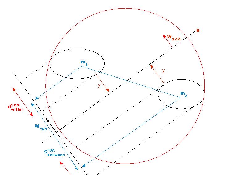
Figure 1: Between and within-class distances for FDA, SVM, and metric-learning-based SVM. While FDA’s between-class distance, $s^{FDA}_{between}$, considers the two sample means $\mathbf{m}_{1}$ and $\mathbf{m}_{2}$, standard SVM and metric-learning-based SVM’s between-class distance, $d^{SVM}_{between}$, i.e $2\gamma$, considers the two nearest instances of two classes with respect to the hyperplane. The outer sphere is the smallest data enclosing sphere, its radius is a measure of the total data scatter which is minimized by the different radius-margin based SVM variants; its minimization together with the margin maximization indirectly minimizes the within-class distances. $d^{SVM}_{within}$ is an example of the measure of the within-class distance of metric-learning-based SVM.

Thus, we see that from the metric learning perspective both FDA and SVM learn a diagonal transformation $\mathbf{W}$. However, the way they define their between and within-class distances is different, although all these distances are based on distances from the fixed hyperplane $H_{1}$ and are defined globally. The FDA between-class distance is the squared distance between the two class means, with respect to the hyperplane $H_{1}:\boldsymbol{1}^{T}\mathbf{x}=0$, while the SVM between-class distance is the minimum distance between two instances of the two classes, with respect to $H_{1}$. On the other hand, FDA defines its within-class distances as the total sum of distances between each instance and its corresponding class mean, while standard SVM ignores the within-class distances, i.e there is no constraint on the pairwise distances of the same class instances. Similar to SVM, metric-learning based SVM defines its between-class distance as the margin; in addition, it defines its within-class distance in different ways. Radius-margin based SVMs [14, 19, 8], which are some instantiations of metric-learning based SVM, use the radius of the smallest sphere as a measure of data spread instead of explicitly defining the within-class distance. Figure 1 graphically depicts the difference between standard SVM, metric-learning based SVM, and FDA.

The metric-learning-based SVM algorithms optimize both the margin and some measures of the within-class distances. Still the constraints on the pairwise distances of the metric-learning-based SVM are a simple version of (4). Their within-class distances are defined globally, with respect to a hyperplane. Their between-class distance, the margin, only takes into account the closest instances of the two classes.

Metric learning algorithms in general follow the within and between-class distances optimization. However they focus more on details, i.e pairwise distances are computed locally, unlike FDA or SVM which focus on global properties of the pairwise distances using the class means or the instances on the margin.

The derivation of generalization error bounds for the presented metric learning problems is an open issue. To the best of our knowledge no such bounds exist. Through the unified view of metric learning and SVM we want to use the error bounds of the latter to derive new bounds for the methods that we present here.

VI A metric-learning based MKL framework

In this section we will show how to exploit the metric-learning approach in the context of MKL. We first show how to formulate $MKL_{\gamma}$ as a metric learning problem with the help of two linear transformations. We proceed by developing a metric-learning-based MKL framework which optimizes both the margin and some measure of the within-class distance using multiple kernels.

VI-A MKL from a metric learning perspective

In MKL we learn linear combinations of kernels of the form $\mathbf{K}_{\boldsymbol{\mu}}=\sum_{k}^{m}\mu_{k}\mathbf{K}_{k}$. The feature space $\mathcal{H}_{\boldsymbol{\mu}}$ that corresponds to the learned kernel $\mathbf{K}_{\boldsymbol{\mu}}$ is given by the mapping:

$${\mathbf{x}}\rightarrow\mathbf{\Phi}_{\boldsymbol{\mu}}({\mathbf{x}})=(\sqrt{\mu_{1}}\mathbf{\Phi}^{T}_{1}({\mathbf{x}}),...,\sqrt{\mu_{m}}\mathbf{\Phi}^{T}_{m}({{\mathbf{x}}}))^{T}$$

$$\in{\mathcal{H}_{\boldsymbol{\mu}}}=\mathbf{D}_{\sqrt{\boldsymbol{\mu}}}\boldsymbol{\Phi}({\mathbf{x}})$$ (21)

where $\mathbf{\Phi}_{k}({\mathbf{x}})$ is the mapping to the $\mathcal{H}_{k}$ feature space associated with the $K_{k}$ kernel, $\boldsymbol{\Phi}({\mathbf{x}})=(\mathbf{\Phi}^{T}_{1}({\mathbf{x}}),...,\mathbf{\Phi}^{T}_{m}({{\mathbf{x}}}))^{T}\in{\mathcal{H}}$, and $\mathbf{D}_{\sqrt{\boldsymbol{\mu}}}$ is block diagonal matrix with block diagonal elements ${\sqrt{\boldsymbol{\mu}}}$.

Similar to SVM, we can also use the fixed hyperplane $H_{1}$ and view $MKL_{\gamma}$ as learning a block diagonal linear transformation $\mathbf{D}_{\sqrt{\boldsymbol{\mu}}}$ in the concatenation feature space $\cal H$, followed by a diagonal linear transformation $\mathbf{W}$ and a translation $b$, such that the margin with respect to the $H_{\boldsymbol{1}}$ hyperplane is maximized and the two classes are placed symmetrically in the two different sides of $H_{\boldsymbol{1}}$. The linear transformation $\mathbf{A}$ associated with $MKL_{\gamma}$ is given by $\mathbf{A}=\mathbf{W}\mathbf{D}_{\sqrt{\boldsymbol{\mu}}}$. So $MKL_{\gamma}$ is also a Mahalanobis metric learning problem where the transformation matrix is $\mathbf{A}=\mathbf{W}\mathbf{D}_{\sqrt{\boldsymbol{\mu}}}$.

From a metric learning perspective SVM uses a single diagonal matrix transformation given by $\mathbf{W}$ and $MKL_{\gamma}$ uses two diagonal matrix transformations given by $\mathbf{W}^{\prime}=\mathbf{W}\mathbf{D}_{\sqrt{\boldsymbol{\mu}}}$; both optimize the same cost function (i.e the margin). A formal comparison of the two methods under the metric-learning view can be found in the Appendix.

VI-B MKL and the optimization of the within-class distance

Similar to SVM, standard $MKL_{\gamma}$ optimizes only the margin, i.e the between-class distances but ignores the within-class distances. As before with SVM we will now develop a metric-learning-based MKL framework in which we will optimize both the margin and some measure of the within-class distances. We will give two examples of metric-learning-based MKL algorithms, using the $SVM_{m}$, section IV-B1, and $\epsilon$-SVM[9].

The $SVM_{m}$ optimization problem, equation (14), in the MKL context becomes:

$$\min_{{\mathbf{w}},b,\boldsymbol{\mu},\boldsymbol{\xi},\boldsymbol{\eta}} \|{\mathbf{w}}\|_{2}^{2}+\frac{C_{1}}{2}\sum_{i}^{n}\xi_{i}+\frac{C_{2}}{2}\sum_{i}^{n}\eta_{i}$$

$$s.t. 1-\xi_{i}\leq y_{i}(\mathbf{W}\mathbf{D}_{\sqrt{\boldsymbol{\mu}}}\mathbf{\Phi}({\mathbf{x}}_{i})+b)\leq 1+\epsilon+\eta_{i},\forall i$$

$$\|\boldsymbol{\mu}\|_{1}=1,\mu_{k}\geq 0,\forall k,\epsilon\geq 0$$

which is equivalent to:

$$\min_{{\mathbf{w}},b,\boldsymbol{\xi},\boldsymbol{\mu},\boldsymbol{\eta}} \frac{1}{2}\sum_{k}^{M}\frac{\langle{\mathbf{w}}_{k},{\mathbf{w}}_{k}\rangle}{\mu_{k}}+\frac{C_{1}}{2}\sum_{i}^{n}\xi_{i}+\frac{C_{2}}{2}\sum_{i}^{n}\eta_{i}$$ (22)

$$s.t. 1-\xi_{i}\leq y_{i}(\sum_{k}^{M}\langle{\mathbf{w}}_{k},\mathbf{\Phi}_{k}({\mathbf{x}}_{i})\rangle+b)\leq 1+\epsilon+\eta_{i}$$

$$\sum_{k=1}^{M}\mu_{k}=1,\mu_{k}\geq 0,\forall k,\xi_{i}\geq 0,\eta_{i}\geq 0,\forall i$$

This optimization problem is the counterpart of $SVM_{m}$ in the MKL context; we will call it $MKL_{m}$. As it was the case with $SVM_{m}$ where setting $\epsilon$ to zero leads to $\epsilon$-SVM, here too, if in the $MKL_{m}$ optimization problem (22), we set $\epsilon=0$ the resulting optimization problem, which we denote by $\epsilon$-MKL, will correspond to the coupling of $\epsilon$-SVM with MKL. $\epsilon$-MKL thus learns kernel combinations that maximize the margin and minimize the within-class distance as the latter is measured by the sum of the distances from the margin hyperplanes.

The $MKL_{m}$ optimization problem, equation (22), is convex and equivalent to:

$$\min_{\boldsymbol{\mu}}J(\boldsymbol{\mu}),\,\,\,\,\,\,\,\,\,\,\,\,s.t.\,\,\,\,\sum_{k=1}^{m}\mu_{k}=1,\mu_{k}\geq 0,\forall k\$$ (23)

where:

$$J(\boldsymbol{\mu})=\left\{\begin{array}[]{ll}\min_{\mathbf{w},b,\boldsymbol{\xi},\boldsymbol{\eta}}&\frac{1}{2}\sum_{k}^{m}\frac{\langle\mathbf{w}_{k},\mathbf{w}_{k}\rangle}{\mu_{k}}+\frac{C_{1}}{2}\sum_{i}^{n}\xi_{i}+\frac{C_{1}}{2}\sum_{i}^{n}\eta_{i}\\ s.t.&1-\xi_{i}\leq y_{i}(\sum_{k}^{m}\langle\mathbf{w}_{k},\mathbf{\Phi}_{k}(\mathbf{x}_{i})\rangle+b)\\ &\,\,\,\,\,\,\,\,\,\,\,\,\,\,\,\,\,\,\,\,\,\,\,\,\,\,\,\,\,\,\,\,\,\,\,\,\,\,\,\,\,\,\,\,\,\leq 1+\epsilon+\eta_{i}\\ &\forall\xi_{i}\geq 0,\forall\eta_{i}\geq 0\end{array}\right.$$ (26)

We can solve it by a two step algorithm, similar to the one used in SimpleMKL [20]. At the first step of the algorithm we fix $\boldsymbol{\mu}$. With fixed $\boldsymbol{\mu}$, problem (22) becomes a SVM-like optimization problem. In the second step, with the optimal values computed by the SVM-like problem in the first step, we optimize the whole problem by gradient descent with respect to $\boldsymbol{\mu}$. The gradient of $J(\boldsymbol{\mu})$ is: $\frac{\partial J(\boldsymbol{\mu})}{\partial\mu_{k}}=-\frac{1}{2}\sum_{ij}(\alpha_{i}^{*}-\beta_{i}^{*})(\alpha_{j}^{*}-\beta_{j}^{*})y_{i}y_{j}K_{k}(\mathbf{x}_{i},\mathbf{x}_{j})$ where $\alpha^{*},\beta^{*}$ are the solution of the first step.

VII Experiments

We performed two sets of experiments. In the first we examined the performance of three metric-learning-based SVM algorithms, namely $SVM_{m}$ (14), $\epsilon$-SVM (6) [9], and SVM-FDA (18) [25]. Note that $\epsilon$-SVM is a special case of $SVM_{m}$ when $\epsilon$ is set to zero. We used as baseline the performance of standard SVM and FDA. We used the stprtool toolbox [11] for FDA. In the second set, we compared the two metric-learning-based MKL algorithms, i.e. $MKL_{m}$ and $\epsilon$-MKL, with SimpleMKL [20], a state-of-the-art $MKL_{\gamma}$ algorithm.

We experimented with UCI benchmark datasets. We first standardized the data to a zero mean and one variance. We examine the performance of the different SVM based methods over the four following kernels: linear, polynomial with degree 2 and 3, and a Gaussian kernel with $\sigma=1$. Kernel $\mathbf{K}$ was normalized as follows: $\mathbf{K}_{ij}={\mathbf{K}_{ij}}/\sqrt{\mathbf{K}_{ii}\mathbf{K}_{jj}}$. For the MKL methods, we learned combinations of the following 20 kernels: 10 polynomial with degree from one to ten, ten Gaussian with bandwidth $\sigma\in\{0.5,1,2,5,7,10,12,15,17,20\}$, the same set of basic kernels as the one used in SimpleMKL [20].

Note that SVM-FDA  can be only applied on the original feature space since it does not have a kernelized version. For $SVM_{m}$, $\epsilon$-SVM, $MKL_{m}$, $\epsilon$-MKL we set $C_{2}$ to $C_{1}/3$, as we can tolerate more bandwidth than margin violations. For $SVM_{m}$  $\epsilon$ is set to three, i.e. the allowed band is three times wider than the margin. The optimal parameter $C$ or $C_{1}$ of the margin slack variables is chosen by an inner 10-fold cross-validation, from the set of $\mathbf{C}=\{0.1,1,10,100,1000\}$. For SVM-FDA we choose $C$ and $\lambda$ from the same set of $\{0.1,1,10,100,1000\}$ using the 10-fold inner cross-validation. We estimated the classification error using 10-fold cross validation. Folds are the same for all algorithms.

The results for the SVM algorithms are given in Table I and for the MKL ones in Table II. We can see that $SVM_{m}$ has the lowest error in most of the cases. Among the 28 different experiments performed for each algorithm (7 datasets $\times$ 4 kernels), $SVM_{m}$ has the lowest error 19 times, $\epsilon$-SVM 10 times, SVM 5 times and FDA never. We should note that the second constraint of both $\epsilon$-SVM (7) and $SVM_{m}$ (14) will not be triggered if the data points are already very close to the margin; in such case $SVM_{m}$ and $\epsilon$-SVM have the same performance as SVM. We also compared the statistical significance of the performance difference using a McNemar’s test with the significance level set at 0.05. For each experiment of a given algorithm, i.e. kernel and dataset, the algorithm was credited with one point if it was significantly better than another algorithm for the same experiment, half a point if there was no significance difference between the two algorithms, and no point if it was significantly worse than the other algorithm. Under this ranking schema, in the original feature space, $SVM_{m}$ got a total score of 20.5 points over the seven datasets, out of a total possible maximum of 28, followed by SVM-FDA with 17, SVM with 15, $\epsilon$-SVM with 14; FDA is by far the worst with only 3.5 points. In the polynomial kernel space of degree two and three, $SVM_{m}$ and $\epsilon$-SVM rank first with 14.5 points but their advantage over SVM which got 13 points is not so pronounced; FDA got zero points. With the gaussian kernel, both $SVM_{m}$ and $\epsilon$-SVM have a significant advantage over SVM and FDA; the former two got 14.5 points while SVM and FDA got only six and seven points respectively. Overall $SVM_{m}$ has a consistent advantage over the different datasets and the different kernels we experimented with. We should note here that the incorporation of the within-class distance in the optimization problem seems to bring the largest benefit when the kernel that is used is not that appropriate for the given problem, e.g. the Gaussian kernel for the datasets we experimented with here, this advantage is not so pronounced when the chosen kernel is good, e.g. polynomial of degree two and three. In other words incorporating the within-class distance seems to have a corrective effect when a mediocre or poor kernel is used.

TABLE I: 10-fold CV classification error for $SVM_{m}$, $\epsilon$-SVM, SVM-FDA, SVM and FDA. Note that SVM-FDA can be applied only in the original feature space, but not in the kernel spaces. A bold entry indicates that the respective method had the lowest classification error.

Kernel	Datasets	$SVM_{m}$	$\epsilon$-SVM	SVM-FDA	SVM	FDA	Kernel	Datasets	$SVM_{m}$	$\epsilon$-SVM	SVM	FDA
	sonar	21.63	23.08	20.67	32.69	27.88		sonar	13.46	12.98	13.46	26.44
	wpbc	19.7	21.21	22.73	25.25	26.77		wpbc	20.2	20.71	20.2	48.48
	ionosphere	9.12	11.97	10.26	7.98	64.1		ionosphere	5.98	6.27	6.27	30.48
Linear	wdbc	2.11	3.69	2.99	2.28	3.87	poly3	wdbc	2.64	2.28	2.64	62.74
	liver	30.43	31.3	30.72	31.01	39.13		liver	28.7	30.43	29.57	40.29
	musk1	13.03	15.76	13.24	17.02	20.8		musk1	4.2	4.83	4.2	36.36
	ovarian	4.35	4.35	3.95	4.35	48.22		ovarian	9.49	9.49	19.37	64.03
Score	McNemar	20.5	14	17	15	3.5	Score	McNemar	14.5	14.5	13	0
	sonar	17.79	17.31		19.23	41.83		sonar	34.62	34.62	42.79	42.79
	wpbc	23.74	23.74		24.24	41.83		wpbc	23.74	23.74	23.74	23.74
	ionosphere	5.41	5.98		5.98	32.76		ionosphere	5.41	5.41	10.82	8.26
Poly2	wdbc	3.51	4.75		3.51	58.52	gauss1	wdbc	6.5	6.85	16.34	10.54
	liver	30.14	29.86		30.72	39.98		liver	32.17	32.46	32.17	40.29
	musk1	6.09	6.93		6.3	50.84		musk1	39.92	39.92	43.49	43.07
	ovarian	9.09	9.09		15.81	64.03		ovarian	35.97	35.97	35.97	35.97
Score	McNemar	14.5	14.5		13	0	Score	McNemar	14.5	14.5	6	7

The poor performance of FDA can be explained by the between-class distance measure it deploys. Using the class means as a between-class distance measure can lead to class overlapping. $\epsilon$-SVM, $SVM_{m}$ and SVM-FDA do not have this problem since they use the margin as the between-class distance. Unlike SVM-FDA which can be applied only in the original feature space, since it cannot be kernelized, both $\epsilon$-SVM and $SVM_{m}$ can be easily kernelized.

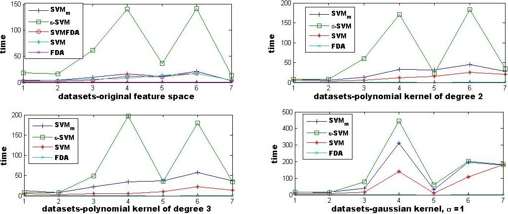
Figure 2: Running time of $SVM_{m}$, $\epsilon$-SVM, SVM-FDA, SVM and FDA. Datasets are in the same order as in Table I.

In Figure 2 we give the running times of the different methods. These are in agreement with our remarks in IV-B. $\epsilon$-SVM is the slowest since in general the closer $\epsilon$ is to zero, the more constraints are active and the slower the algorithm will be. FDA is the fastest one but as we saw its predictive performance is quite poor.

In Table  II we give the results for the MKL experiments. $\epsilon$-MKL and $MKL_{m}$  have now only a slight advantage compared to SimpleMKL. $\epsilon$-MKL has the lowest error in six datasets while $MKL_{m}$ is the best in two datasets. In terms of the McNemar score, $MKL_{m}$ got 8.5 points, followed by $\epsilon$-MKL with eight points and SimpleMKL with 7.5 points. Unlike standard SVM the incorporation of the within-class distance in the MKL cost function does not seem to deliver a significant performance improvement. This is somehow in agreement with our previous observation, i.e. that the incorporation of the within-class distance measure seems to have a strong positive effect when the kernel that is used is not appropriate. By learning the kernel as MKL does we overcome the problem of a possible poor kernel selection, provided that within the kernel set over which we learn there are appropriate kernels for the given problem.

TABLE II: 10-fold CV classification error for SimpleMKL, $MKL_{m}$ and $\epsilon$-MKL. A bold entry indicates that the respective method had the lowest classification error. An italic entry indicates that the respective methods had a lower error than SimpleMKL

Datasets	# Instances	# Features	SimpleMKL	$MKL_{m}$	$\epsilon$-MKL
Sonar	208	60	16.35	13.46	12.5
Ionosphere	351	34	4.27	3.70	3.99
Musk1	476	166	5.25	4.41	4.20
Wdbc	569	30	2.64	2.11	2.64
Stroke	208	2810	23.08	22.60	22.12
Ovarian	253	771	4.35	4.35	3.95
Liver	354	6	34.20	34.49	32.46
Wpbc	198	34	23.23	22.73	22.73
Score McNemar			7.5	8.5	8

From the results, it is apparent that one does not need only to control for the between-class distance, as standard SVM does, but also for the within-class distance, since the incorporation of some measure of the latter in the optimization problem considerably improves the performance over the standard SVM. When it comes to determining which within-class distance measure is more appropriate then the width of the band containing the instances that we deployed in $SVM_{m}$ has a clear advantage since it does not only lead to the best performance but it results in a convex optimization problem which is easy to kernelize and in addition includes as a special case $\epsilon$-SVM.

VIII Conclusion

Inspired by recent work that investigated the relations of SVM and metric learning [9], we present here a novel framework that equips SVM, as well as MKL, with metric learning concepts. The new algorithms that we propose optimize not only the standard SVM margin, which can be seen as a measure of the between-class distance, but in addition they also optimize measures of the within-class distance. For the latter we propose a new measure, the width of the band along the margin hyperplane that contains the learning instances, and we derive new SVM and MKL variants that exploit. Our experimental results show that we achieve important predictive performance improvements if we include measures of the within-class distance in the optimization problem. In addition the new algorithms that we derived are convex and easy to kernelize.

There are a number of additional issues we plan to examine. The most challenging one is the derivation of generalization error bounds for the presented metric learning problems. To the best of our knowledge no such bounds exist for metric learning. Through the unified view of SVM and metric learning we want to relate the SVM error bound with the presented metric learning problems. It is also a challenge to determine which measures of between and within-class distances are the best for a specific problem. Additionally, and similar to [2] and [10], we want to solve for the full regularization path, for $\epsilon$ or $\lambda$.

Appendix

We here present a formal comparison of SVM and $MKL_{\gamma}$  under the metric-learning view.

From a metric learning perspective SVM uses a single diagonal matrix transformation given by $\mathbf{W}$ and $MKL_{\gamma}$ a two diagonal matrix transformation given by $\mathbf{W}^{\prime}=\mathbf{W}\mathbf{D}_{\sqrt{\boldsymbol{\mu}}}$; both optimize the same cost function (i.e the margin). We will compare SVM and $MKL_{\gamma}$ by comparing the use of one and two diagonal transformation matrices.

For $MKL_{\gamma}$ the $\mathbf{D}_{\sqrt{\boldsymbol{\mu}}}$ matrix is block diagonal, while if we use that decomposition with SVM it is a simple diagonal matrix. We denote by $\mathbf{w}=diag({\mathbf{W}})$, $\mathbf{w}^{\prime}=diag(\mathbf{W}^{\prime})$ and $\sqrt{\boldsymbol{\mu}}=diag(\mathbf{D}_{\sqrt{\boldsymbol{\mu}}})$. The optimization problems of SVM and $MKL_{\gamma}$ can be formulated as follows:

$$\text{SVM:}\max_{\mathbf{w},b} \gamma$$ (27)

$$s.t y_{i}(\mathbf{w}^{T}\mathbf{x}_{i}+b)\geq\gamma,\forall i$$

$$\|\mathbf{w}\|_{p}=1$$

$$\text{MKL:}\max_{\mathbf{w^{\prime}},b} \gamma$$ (28)

$$s.t y_{i}((\mathbf{w^{\prime}}\circ\boldsymbol{\mu})^{T}\mathbf{x}_{i}+b)\geq\gamma,\forall i$$

$$\|\mathbf{w^{\prime}}\|_{p}=1,\,\,\|\boldsymbol{\mu}\|_{p}=1,\mu_{i}\geq 0$$

We now try to highlight relationship of these two optimization problems. Given some $\boldsymbol{\mu}$ vector such that $\mu_{i}\neq 0,\forall i$, $\|\boldsymbol{\mu}\|_{p}=1$, and $\mathbf{w}=\mathbf{w^{\prime}}\circ\boldsymbol{\mu}$, we define a new norm $l_{\boldsymbol{\mu}}(\mathbf{w})$ as follows: $l_{\boldsymbol{\mu}}(\mathbf{w})=\|\mathbf{w^{\prime}}\|_{p}$. It is easy to prove that $l_{\boldsymbol{\mu}}({\mathbf{w}})$ satisfies all the properties of a norm, which means it is a valid norm.

Using this new norm, we can rewrite problem (28) as:

$$\max_{\mathbf{w},b}\,\,\,\gamma \,\,\,\,\,\,s.t.\,\,\,\,\,y_{i}(\mathbf{w}^{T}\mathbf{x}_{i}+b)\geq\gamma,\forall i$$

$$\,\,\,\,\,\,\,l_{\boldsymbol{\mu}}(\mathbf{w})=1,\,\,\|\boldsymbol{\mu}\|_{p}=1$$

Let $T_{\mathbf{w}}$ be the feasible set of $\|\mathbf{w}\|_{p}=1$, obviously $T_{\mathbf{w}}$ is also the feasible set $\|\mathbf{w^{\prime}}\|_{p}=1$; $T_{\boldsymbol{\mu}}$ is the feasible set of $\|\boldsymbol{\mu}\|_{p}=1$. Let $T_{\mathbf{w^{\prime}}\circ\boldsymbol{\mu}}=\{\mathbf{w^{\prime}}\circ\boldsymbol{\mu}|\boldsymbol{\mu}\in T_{\boldsymbol{\mu}},\mathbf{w^{\prime}}\in T_{\mathbf{w}}\}$. For a given value of $\boldsymbol{\mu}=\boldsymbol{c}$ there is a one-to-one mapping from $T_{\mathbf{w}}$ to $T_{\mathbf{w}^{\prime}\circ\boldsymbol{\mu}=\boldsymbol{c}}$. The cardinality of the $T_{\mathbf{w}}$ feasible set is much smaller than the cardinality of $T_{\mathbf{w}^{\prime}\circ\boldsymbol{\mu}}$ therefore using this new norm gives more flexibility in finding a solution of the optimization problem, which could potentially lead to a better solution.

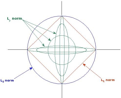
Figure 3: Relation of $L_{1}$, $L_{2}$ and $L_{\boldsymbol{\mu}}$ norms

In Figure 3 we illustrate the relations of the different norms just discussed in the two dimensional space. We compare the p=1 and p=2 norms of $\mathbf{w}$ to its $l_{\boldsymbol{\mu}}$ norm. We fix $\|\mathbf{w}\|_{1}=1$, its feasible set $T_{\mathbf{w}}$ is the diamond, $\|\mathbf{w}\|_{2}=1$, its feasible set $T_{\mathbf{w}}$ is the outer circle, and $l_{\boldsymbol{\mu}}(\mathbf{w})=1$, $\|\boldsymbol{\mu}\|_{1}=1$, for which we have the set of feasible sets, $T_{\mathbf{w}^{\prime}\circ\boldsymbol{\mu}}$, that correspond to the different values of $\boldsymbol{\mu}$ that satisfy $\|\boldsymbol{\mu}\|_{1}=1$, which are given by the inner ellipsoids.

References

- [1] Argyriou, A., Micchelli, C.A., Pontil, M.: Learning convex combinations of continuously parameterized basic kernels. In: COLT 2005 (2005)
- [2] Bach, F., Thibaux, R., Jordan, M.: Computing regularization paths for learning multiple kernels (2005)
- [3] Cortes, C., Mohri, M., Rostamizadeh, A.: L2 regularization for learning kernels. In: UAI (2010)
- [4] Cortes, C., Mohri, M., Rostamizadeh, A.: Two stage learning kernel algorithms. In: International Conference on Machine Learning (2010)
- [5] Cristianini, N., Shawe-Taylor, J.: An introduction to Support Vector Machines. Cambridge University Press (2000)
- [6] Cristianini, N., Shawe-Taylor, J., Elisseeff, A.: On the extensions of kernel alignment. In: Advances in Neural Information Processing Systems 14. MIT Press (2001)
- [7] Davis, J., Kulis, B., Jain, P., Sra, S., Dhillon, I.: Information-theoretic metric learning. In: Proceedings of the 24th international conference on Machine learning. ACM New York, NY, USA (2007)
- [8] Do, H., Kalousis, A., Hilario, M.: Feature weighting using margin and radius based error bound optimization in svms. In: European Conference on Machine Learning (2009)
- [9] Do, H., Kalousis, A., Wang, J., Woznica, A.: A metric learning perspective of svm - on the relation of svm and lmnn. In: International Conference on Artificial Intelligence and Statistics (2012)
- [10] Efron, B., Hastie, T., Johnstone, I., Tibshirani, R.: Least angle regression. Annals of Statistics (2004)
- [11] Franc, V., Hlavac, V.: Statistical Pattern Recognition Toolbox. Czech Technical University Prague, http://cmp.felk.cvut.cz/cmp/software/stprtool/
- [12] Globerson, A., Roweis, S.: Metric learning by collapsing classes. In: Advances in Neural Information Processing Systems. vol. 18. MIT Press (2006)
- [13] Goldberger, J., Roweis, S., Hinton, G., Salakhutdinov, R.: Neighbourhood components analysis. In: Advances in Neural Information Processing Systems. vol. 17. MIT Press (2005)
- [14] J.Weston, S.Mukherjee, O.Chapelle, M.Pontil, J.Poggio, V.Vapnik: Feature selection for svms. vol. 13, pp. 668–674 (2000)
- [15] Kloft, M., Brefeld, U., Sonnenburg, S., Zien, A.: lp multiple kernel learning. Journal of Machine Learning Research (2011)
- [16] Lanckriet, G., Cristianini, N., Bartlett, P., Ghaoui, L.E.: Learning the kernel matrix with semidefinite programming. Journal of Machine Learning Research 5, 27–72 (2004)
- [17] O.Duda, R., E.Hart, P., Stork, D.G.: Pattern Classification. A Wiley Interscience Publication (2001)
- [18] Ong, C.S., Smola, A.J., Williamson, R.C.: Learning the kernel with hyperkernels. Journal of Machine Learning Research 6, 1043–1071 (2005)
- [19] Rakotomamonjy, A.: Variable selection using svm-based criteria. Journal of Machine Learning Research 3, 1357–1370 (2003)
- [20] Rakotomamonjy, A., Bach, F., Canu, S., Grandvalet, Y.: Simplemkl. Journal of Machine Learning Research 9, 2491–2521 (2008)
- [21] Shivaswamy, P.K., Jebara, T.: Maximum relative margin and data-dependent regularization. Journal of Machine Learning Research 11, 747–788 (2010)
- [22] Sonnenburg, S., Raetsch, G., Christin, Schaefer, Schoelkopf, B.: Large scale multiple kernel learning. Journal of Machine Learning Research 7, 1531–1565 (July 2006)
- [23] Weinberger, K., Saul, L.: Distance metric learning for large margin nearest neighbor classification. The Journal of Machine Learning Research 10, 207–244 (2009)
- [24] Xing, E., Ng, A., Jordan, M., Russell, S.: Distance metric learning with application to clustering with side-information. In: Advances in Neural Information Processing Systems (2003)
- [25] Xiong, T., Cherkassky, V.: A combined svm and lda approach for classifiction. In: IJCNN (2005)