Inelastic neutron scattering studies of YFeO₃

Abstract

Spin waves in the the rare earth orthorferrite YFeO₃ have been studied by inelastic neutron scattering and analyzed with a full four-sublattice model including contributions from both the weak ferromagnetic and hidden antiferromagnetic orders. Antiferromagnetic (AFM) exchange interactions of $J_{1}$= -4.23$\pm$0.08 (nearest-neighbors only) or $J_{1}$ = -4.77$\pm$0.08 meV and $J_{2}$ = -0.21$\pm$0.04 meV lead to excellent fits for most branches at both low and high energies. An additional branch associated with the hidden antiferromagnetic order was observed. This work paves the way for studies of other materials in this class containing spin reorientation transitions and magnetic rare earth ions.

I Introduction

The rare earth orthorferrites RFeO₃ are an important family of materials whose magnetic properties remain a focus of considerable research due to promising applications in innovative spintronic devices.Kimel et al. (2004) Furthermore, they contribute to an emerging class of materials, i.e., multiferroics with strong magnetoelectric (ME) coupling.Eerenstein et al. (2006); Tokunaga et al. (2009) In multiferroic materials, coupling between magnetic and ferroelectric order gives rise to magnetization on application of an electric field or to electric polarization on application of a magnetic field. Their complex non-collinear structures and magnetic phase transitions are due to the combination of the antiferromagnetic (AFM) exchange interaction with the Dzyaloshinsky-Moriya (DM) antisymmetric exchange interaction.Dzyaloshinsky (1958); Moriya (1960)

In general materials in the RFeO₃ family contain two magnetic subsystems consisting of either iron or rare earth ions. With decreasing temperature or an applied magnetic field, most of these materials undergo a spin reorientation transition from $\Gamma_{4}\left(G_{a},F_{c}\right)$, where the net moment is along the c-axis, to $\Gamma_{2}\left(G_{c},F_{a}\right)$, where the net moment is along the a-axis (for notation, see appendix A).White (1969) This transition occurs over a finite temperature range where the spins rotate continuously in the lower symmetry phase $\Gamma_{24}\left(G_{ac},F_{ca}\right)$. No structural change is observed in ErFeO₃ and YbFeO₃, suggesting that this is purely a magnetic transition.Bazaliy et al. (2005); Tsymbal et al. (2005) Rotation of the iron moments leads to a change in the magnitude of the magnetization on the rare earth subsystem, which must be included in the calculation of the rotation angle and absolute magnetization. At lower temperatures an additional magnetic transition occurs when the rare earth moments order.

The nonmagnetic yittrium sublattice in YFeO₃ enables us to focus only on the magnetic interactions of the iron sublattices. The lack of a spin reorientation transition with temperature considerably simplifies the modeling of spin dynamics and makes YFeO₃ a good stepping stone to studying other materials in this class with more complex dynamics.

YFeO₃ adopts an orthorhombic structure with space group Pbnm. Below 640K, YFeO₃ is a non-collinear antiferromagnet whose four Fe³⁺ ions are in the state $\Gamma_{4}(G_{a},F_{c},A_{b})$, shown in Fig. 1. The ratio of $A_{b}/G_{a}$, which determines the canting angle along b, was found to be 1.59(7)$\cdot$10^-2.Plakhty et al. (1983) Values for $F_{c}/G_{a}$ range from 8.9$\cdot$10^-3 to 1.29$\cdot$10^-2 where the lower values may be due to ferromagnetic impurities. These values set limits on the canting angle along c.

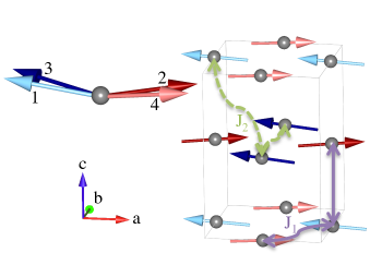
Figure 1: (color online) Magnetic unit cell of YFeO₃, showing only the positions of the Fe³⁺ atoms. The four sublattices show weak ferromagnetism and antiferromagnetism along the c and b directions, respectively. Exchange interactions between nearest ($J_{1}$) and next-nearest ($J_{2}$) neighbors are shown by the solid purple and dashed green arrows, respectively.

Spin waves in similar systems TmFeO₃ and ErFeO₃ were previously measured and modeled with a combination of four-sublattice and two-sublattice models for the short-wavelength and long-wavelength dispersion, respectively.Shapiro et al. (1974) For TmFeO₃, the exchange constant for nearest neighbors only ($J_{2}\equiv 0$ ) was found to be $J_{1}$ = -4.22 meV. With next-nearest neighbors included, the exchange constants were $J_{1}$ = -5.02 meV and $J_{2}$ = -0.324 meV. A four-sublattice model containing only exchange predicts reasonable energies for the observed spin wave branches. The two easy-axis anisotropy parameters are approximately equal near the transition and an additional term proportional to the fourth power of the spin controls the rotation angle over the temperature range of the transition.

TbFeO₃ has generated renewed interest since measurements in an applied magnetic field found an unusual incommensurate phase with a periodic array of widely separated domain walls. The ordering of domain walls is due to a long-range force from the exchange of magnons propagating through the iron sublattice.Artyukhin et al. (2012) Spin waves in TbFeO₃ were previously measured and modeled with a four-sublattice model containing only exchange interactions.Gukasov et al. (1997) In principle, the distortion from cubic symmetry leads to different exchange constants for nearest and next-nearest neighbors within the ab plane and between planes. Measured distances between Fe³⁺ ions are however within 2% and 6% of each other for nearest neighbors and next-nearest neighbors, respectively. In each of these cases, the exchange parameters within the ab plane and between planes can be treated as equal. With only nearest neighbors, $J_{1}$ = -4.34 meV and with both nearest and next-nearest neighbors the exchange constants were $J_{1}$ = -4.95 meV and $J_{2}$ = -0.241 meV.

In YFeO₃, spin waves were measured at 1.4 and 2.2 meV in the long-wavelength limit with Raman scattering at room temperature.White et al. (1982) A two-sublattice model was then used to obtain estimates for the anisotropy constants, defined in Eqn. III, of $K_{a}=4.6\cdot 10^{-3}$ meV and $K_{c}=1.13\cdot 10^{-3}$ meV. In this work, we measured spin waves in YFeO₃ by inelastic neutron scattering on two different energy scales and analyzed them simultaneously with a quantitative model considering contributions from both the weak ferromagnetic and hidden antiferromagnetic orders present in the full four-sublattice model.

II Experiment

Polycrystalline YFeO₃ was prepared by a solid state reaction. Starting materials of Y₂O₃ and Fe₂O₃ with 99.99% purity were mixed and ground followed by a heat treatment in air at 1000-1250^∘C for at least 70 hours with several intermediate grindings. Phase purity of the resulting compound was checked with a conventional x-ray diffractometer. The resulting powder was hydrostatically pressed into rods (8 mm in diameter and 60 mm in length) and subsequently sintered at 1400^∘C for 20 hours.

The crystal growth was carried out using an optical floating zone furnace (FZ-T-10000-H-IV-VP-PC, Crystal System Corp., Japan) with four 500W halogen lamps as heat sources. The growing conditions were: the growth rate was 5 mm/hour, the feeding and seeding rods were rotated at about 15 rpm in opposite directions to ensure the liquid’s homogeneity and an oxygen and argon mixture at 1.5 bar pressure was applied during growth. Lattice constants in the Pbnm space group were $a=5.282$ Å, $b=5.596$ Å, and $c=7.605$ Å. The sample was orientated in the (H0L) plane for neutron measurements.

Inelastic neutron scattering measurements were done using the Cold Neutron Chopper Spectrometer (CNCS)Ehlers et al. (2011) and the Fine Resolution Chopper Spectrometer (SEQUOIA)Granroth et al. (2006, 2010) at the Spallation Neutron Source (SNS) at Oak Ridge National Laboratory. The data were collected using fixed incident neutron energies 99.34 meV (SEQUOIA) and 3.15 meV (CNCS), which allowed for the measurement of excitations up to energy transfers of $\Delta\omega\sim$ 80 meV (SEQUOIA) and 2.5 meV (CNCS). In these configurations, a full width at half maximum (FWHM) resolution of 5.5 meV (SEQUOIA) and 0.06 meV (CNCS) was obtained at the elastic position. The sample was cooled to 4 K on SEQUOIA and base temperature ($<2$ K) on CNCS. The MantidPlot Man (2012) and DAVE Azuah et al. (2009) software packages were used for data reduction and analysis.

III Theoretical Modeling of Spin Waves

Our model Hamiltonian, given in Eqn. III, contains isotropic exchange constants $J_{1}$ and $J_{2}$ coupling nearest-neighbor and next-nearest-neighbor Fe³⁺ spins, two DM antisymmetric exchange constants $D_{1}$ and $D_{2}$ responsible for the canting along c and b and two easy-axis anisotropy constants $K_{a}$ and $K_{c}$ along the a and c axes.

$$H= -J_{1}\sum_{\left<i,j\right>}\boldsymbol{S}_{i}\cdot\boldsymbol{S}_{j}-J_{2}\sum_{\left<i,j\right>^{\prime}}\boldsymbol{S}_{i}\cdot\boldsymbol{S}_{j}$$

$$-D_{1}\sum_{\boldsymbol{R}_{j}=\boldsymbol{R}_{i}+a\left(\hat{x}\pm\hat{y}\right)}\hat{y}\cdot\boldsymbol{S}_{i}\times\boldsymbol{S}_{j}$$

$$-D_{2}\sum_{\boldsymbol{R}_{j}=\boldsymbol{R}_{i}+a\left(\hat{x}\pm\hat{y}\right)}\hat{z}\cdot\boldsymbol{S}_{i}\times\boldsymbol{S}_{j}$$

$$-K_{a}\sum_{i}\left(\boldsymbol{S}_{i}^{x}\right)^{2}-K_{c}\sum_{i}\left(\boldsymbol{S}_{i}^{z}\right)^{2}$$ (1)

The DM interaction was only considered among nearest neighbors within the ab plane, which is the minimum necessary to explain the canting of all four sublattices. A third DM interaction is possible along $b$ with nearest neighbors between planes, but is not needed to describe the spin structure and would add additional complexity to our model.

Each of the four spins are written in spherical coordinates as

$$\boldsymbol{S_{i}}=S\left(\textrm{sin}\,\theta_{i}\,\textrm{cos}\,\phi_{i},\textrm{sin}\,\theta_{i}\,\textrm{sin}\,\phi_{i},\textrm{cos}\,\theta_{i}\right)$$ (2)

where $S=5/2$. As a first step in this analysis, one must find the angles associated with the minimum classical energy. By assuming that $\theta_{i}=\theta$ for all sublattices and $\phi_{1}=\pi+\phi$, $\phi_{2}=\phi$, $\phi_{3}=\pi-\phi$, and $\phi_{4}=2\pi-\phi$, the number of independent angles is reduced to two. Assuming small angles, one can linearize the problem and find the expressions in Eqn. 3 and Eqn. 4 for $\theta$ and $\phi$ to lowest order as a function of $J_{1}$, $J_{2}$, $D_{1}$, $D_{2}$, $K_{a}$ , and $K_{c}$.

$$\theta =\frac{\pi}{2}+\frac{2D_{1}}{6J_{1}+K_{c}-K_{a}}$$ (3)

$$\phi =-\frac{2D_{2}}{4J_{1}-8J_{2}-K_{a}}$$ (4)

In the above expressions, $\theta\leq\frac{\pi}{2}$ and $\phi>0$. Next these expressions were then used to find values for $D_{1}$ and $D_{2}$ that produce the experimentally determined canting angles. The ratio of $F_{c}/G_{a}$ = 1.29$\cdot$10^-2 and $A_{b}/G_{a}$ = 1.59$\cdot$10^-2 were used to fix the angles $\theta=$ 1.5656 (89.70^∘) and $\phi=$ 0.0032 (0.18^∘).Plakhty et al. (1983)

The inelastic neutron cross section for undamped spin waves is

$$S\!\left(\boldsymbol{q},\omega\right) =\sum_{\alpha,\beta}\left(\delta_{\alpha\beta}-q_{\alpha}q_{\beta}/q^{2}\right)S_{\alpha\beta}\!\left(\boldsymbol{q},\omega\right)$$ (5)

$$=\sum_{n,\alpha}\left[1-(q_{\alpha}/q)^{2}\right]\delta(\omega-\omega_{n}(\boldsymbol{q}))S^{(n)}_{\alpha\alpha}\!\left(\boldsymbol{q}\right)$$ (6)

where $\alpha$ and $\beta$ are the cartesian directions $x,y,z$ and $n$ enumerates the individual branches.Shirane et al. (2004) $S_{\alpha\beta}\!\left(\boldsymbol{q},\omega\right)$ is the spin-spin correlation function describing undamped spin waves at low temperature. The spin-spin correlation function is diagonal when there is no net moment and antisymmetric otherwise, meaning that off-diagonal elements do not contribute to the intensity. The energies $\omega_{n}(\boldsymbol{q})$ and terms contributing to the scattering intensities $S^{(n)}_{\alpha\alpha}\!\left(\boldsymbol{q}\right)$ were solved using the 1/S formalism outlined in Ref. Haraldsen and Fishman, 2009 and appendix A of Ref. Fishman et al., 2013. For direct comparison with experimental intensities, the effects of the magnetic form factor, instrumental resolution function, and integration width were included in our calculations according to appendix B.

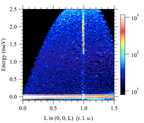
Figure 2: (color online) Spin wave energy gap in YFeO₃ measured by inelastic neutron scattering.

To find the set of parameters that best fits the data, the energy with the highest intensity was taken at eight points in reciprocal space that described the shape of the spin wave dispersion. Our model finds two branches with similar energies contributing to the highest intensity branch. Energy differences range from 0.8 meV at the zone center to 0.01 meV at the zone boundary. These branches are, however, too close in energy to be resolved separately in the cuts shown in Figs. 3c and 3d, so the energy bin with the highest intensity was compared against the average of the two energies weighted by their intensities.

At the zone center we used the observed energies from Ref. White et al., 1982 of 1.4 and 2.2 meV. The lower value is in good agreement with measurements from CNCS shown in Fig. 2, though we were not able to independently verify the frequency of the second mode. The variance was estimated by a Gaussian fit to the measured data. Exchange and anisotropy parameters $J_{1},J_{2},K_{a}$ and $K_{c}$ were fitting parameters, $D_{1}$ and $D_{2}$ were adjusted for each calculation using Eqn. 3 and the canting angles $\theta$ an $\phi$ remained fixed. The NLopt nonlinear-optimization packageJohnson was used for the least squares fitting. Error bars indicate when the reduced $\raisebox{1.50696pt}{$\chi$}^{2}$ increases by 1.0. For $D_{1}$ and $D_{2}$ we propagated the error assuming a 10% error in the canting angles.

Table 1: Best fit parameters used in this work and compared with other work on YFeO₃ and similar materials. In the second line only nearest neighbors were included (J₂=0.0). All values are in meV

Material	Num. SL	$J_{1}$	$J_{2}$	$D_{1}$	$D_{2}$	$K_{a}$	$K_{c}$
YFeO3	4	-4.77$\pm$0.08	-0.21$\pm$0.04	0.074$\pm 0.008$	0.028$\pm$0.003	0.0055$\pm$0.0002	0.00305$\pm$0.0002
	4	-4.23$\pm$0.08	0.0	0.066$\pm$0.007	0.028$\pm$0.003	0.0063$\pm$0.0002	0.0036$\pm$0.0002
YFeO3White et al. (1982)	2	-4.96	0.0	0.11		0.0046	0.0011
TmFeO3Shapiro et al. (1974)	4	-5.01	-0.32
	4	-4.22	0.0
TbFeO3Gukasov et al. (1997)	4	-4.94	-0.24
	4	-4.34	0.0

Parameters determined from this fit along with data from similar work on YFeO₃ and similar materials is given in Tbl. 1. Values for $J_{1}$ are considerably lower than those published by White et al., possibly because their fit considered only the long wavelength limit. Our results are similar to those of Shapiro et al.Shapiro et al. (1974) and Gukasov et al.Gukasov et al. (1997) in similar materials. Anisotropy parameters are not equal in the 2-sublattice and 4-sublattice models because the hidden canting is absorbed into renormalized anisotropy parameters.Herrmann (1964) Therefore anisotropy parameters should not be directly compared between two and four sublattice models.

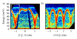
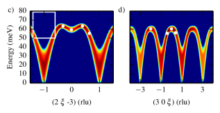
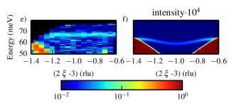
Figure 3: (color online) Measured spin wave dispersion along a) $(2,\xi,{-3})$ and b) $(3,0,\xi)$ and calculated spin wave dispersion along c) $(2,\xi,{-3})$ and d) $(3,0,\xi)$. The background contains phonon modes not included in our model. e) Enlargement of the region outlined by the white box in a). f) Enlargement on the region outlined by the white box in c) and with the intensity multiplied by 10⁴. In all figures, the white dots show energies used for fitting. Black pixels show regions where no data was collected.

IV Discussion

Overall, excellent fits are obtained for most branches. Figs. 3a and 3c show the measured and calculated spin wave dispersion along (2, $\xi$, -3). Both show a dip in frequency and intensity at (2, 0, -3) and the integration range and experimental resolution explain the line width. The intensity around 70 meV near $\xi$ = -1,1 appears to be magnetic scattering and is not visible in our calculation on this intensity scale. Fig. 3e enlarges the region in Fig. 3a near $\xi$ = -1 outlined by the white box. Spin wave branches in this region are also reported elsewhere.Shapiro et al. (1974); Gukasov et al. (1997) The two-sublattice model does not contain any branches near $\xi$=-1,1 that could explain this intensity. Two-magnon scattering occurs around 120 meV, well above the range of energy transfers we measured.Koshizuka and Hayashi (1988) A full four-sublattice model doubles the unit cell, leading to zone folding and consequently two additional branches close to those energies. The hidden antiferromagnetic order gives these additional branches some intensity, motivating us to model this system with the full four-sublattice model.

When $\phi=0$ this branch has zero intensity, consistent with zone folding in a supercell. A nonzero value of $\phi$ makes sublattices 1,3 and 2,4 unequal and gives this branch some intensity. Fig. 3f shows this same region in our calculation, though with the intensity multiplied by $10^{5}$. At these small angles, changing $D_{2}$, and consequently the $\phi$ angle, has the greatest effect on the intensity of this branch whereas chaining $D_{1}$, or the $\theta$ angle, has little if any effect. The ratio of the intensities of these two branches is more than four orders of magnitude too weak compared to the measured ratio of 0.07. Small changes in these angles alone are not enough to account for this difference. In addition, measured energies are up to 9 meV higher than what would be expected from zone folding. Quantum fluctuations are missing from this model and may have an effect on these energies and intensities.

Agreement remains excellent along other directions. Figs. 3b and 3d show the calculated and measured spin wave dispersion along $\left(3,0,\xi\right)$. Calculated energies agree well with the measured values. The integration range and resolution function accounts for the observed widths, especially at low energies. Aluminum and phonon scattering have not been subtracted and may account for any structure seen in the background.

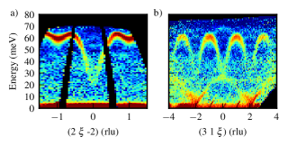
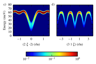
Figure 4: (color online) a) Measured spin wave dispersion along a) (2, $\xi$, -2) and b) (3, 1, $\xi$) and calculated spin wave dispersion along c) (2, $\xi$, -2) and d) (3, 1, $\xi$). The phonon mode with double periodicity was not included in our model. Black pixels show regions where no data was collected.

To show how the spin wave intensities depend on the location in reciprocal space, Figs. 4a and 4c show the calculated and observed spin wave dispersion along (2, $\xi$, -2). Despite identical energies, the intensity is dramatically different from that observed along (2, $\xi$, -3) in Fig. 3. Along ( 2, $\xi$, -2) the intensity approaches the background at low energies and increases dramatically with energy. The change from L = -3 to L=-2 changes the reciprocal lattice points from Q-type, $(h,k,l)$ = (even, odd, odd), to O-type, $(h,k,l)$ = (even, even, even).Shapiro et al. (1974)

Figs. 4b and 4d show the calculated and observed spin wave dispersion along $\left(3,1,\xi\right)$. In this direction the intensity also approaches background at low energies and increases dramatically with energy. The change from K = 0 to K = 1 also changes the reciprocal lattice points from Q-type, $(h,k,l)$ = (odd, even, odd), to O-type, $(h,k,l)$ = (odd, odd, even).

An additional phonon mode is observed below 25 meV with twice the periodicity of the spin wave. The change in periodicity can be explained by the different unit cells corresponding with the crystallographic and magnetic structures. Ignoring small distortions of the yittrium and oxygen atoms from their ideal positions, treating the two iron sublattices as inequivalent atoms doubles the length of the unit cell along c. Views of the powder average show non-dispersive modes at 15, 32, and 82 meV. The intensity of the 15 and 32 meV modes increases with higher Q, suggesting phonon excitations. The 82 meV mode was only measured over a very narrow range in Q that was insufficient to identify its Q-dependence.

V Conclusion

In conclusion, the inelastic spin wave spectrum was measured in the rare-earth orthoferrite YFeO₃ and analyzed with a quantitative model considering contributions from both the weak ferromagnetic and hidden antiferromagnetic orders present in the full four-sublattice model. Excellent fits were obtained that agree well with most observed energies and intensities at both high and low energies. In addition, we observe weak magnetic scattering associated with the hidden antiferromagnetic order along b. Future work will explore changes in the spin wave spectrum with spin reorientation as well as materials where the rare earth also contains magnetic interactions.

Appendix A Symmetry Analysis

The magnetic symmetry of the rare earth orthoferrites is described by linear combinations of the spins on four sublattices. The linear combination $G_{x_{i}}=-\vec{M}_{1}+\vec{M}_{2}-\vec{M}_{3}+\vec{M}_{4}$ describes the primary G-type antiferromagnetic ordering, $F_{x_{i}}=\vec{M}_{1}+\vec{M}_{2}+\vec{M}_{3}+\vec{M}_{4}$ describes the weak ferromagnetism, and $A_{x_{i}}=-\vec{M}_{1}+\vec{M}_{2}+\vec{M}_{3}-\vec{M}_{4}$ describes the weak antiferromagnetism. The subscript $x_{i}$ gives the direction of these vector quantities. In YFeO₃, the G-type antiferromagnetic ordering is along a, the weak ferromagnetism is along c, and the weak antiferromagnetism is along b.

Appendix B Resolution Convolution

For direct comparison with experimental intensities, the effects of the magnetic form factor and the instrumental resolution were included in the calculation. The total intensity is given by

$$I\!\left(\boldsymbol{Q}_{0},\omega_{0}\right)\!=\!\!\int\!\!\!\!\int\!\!F_{Q}^{2}\,S\left(\boldsymbol{Q},\omega\right)R\left(\boldsymbol{Q}\!-\!\boldsymbol{Q}_{0},\omega\!-\!\omega_{0}\right)d\boldsymbol{Q}\,d\omega$$ (7)

where $\boldsymbol{Q}=\boldsymbol{q}+\boldsymbol{G}$ differs by the reciprocal lattice vector $\boldsymbol{G}$ and may be outside the first Brillouin zone. The Fe³⁺ magnetic form factor results in a lower intensity at higher values of $\boldsymbol{Q}$ and can be approximated as $F_{Q}=j_{0}\left(Q\right)$, where $j_{0}\left(Q\right)=A_{0}e^{-a_{0}s^{2}}+B_{0}e^{-b_{0}s^{2}}+C_{0}e^{-c_{0}s^{2}}+D_{0}$ and $s=\mathrm{sin}\theta/\lambda=Q/(4\pi)$. The coefficients are $A_{0}$ = 0.3972 ($a_{0}$ = 13.2442), $B_{0}$ = 0.6295 ($b_{0}$ = 4.9034), $C_{0}$ = -0.0314 ($c_{0}$ = 0.3496) and $D_{0}$ = 0.0044 from Ref. Dianoux and Lander, 2003.

The experiment resolution shape was approximated by a Gaussian encapsulating a simulated resolution volume. For various points along the dispersion, the resolution was calculated using a full model of the incident beam line of SEQUOIAGranroth et al. (2006, 2010) followed by a second model that consists of the Resolution Sample and Resolution Monitor components. Both simulations were performed using the McStasLefmann and Nielsen (1999) Monte Carlo package. First, $36\cdot 10^{10}$ neutron packets were propagated down the incident beamline simulation. Neutron packets that succeeded in making it to the sample position were stored for later use in the secondary spectrometer simulation. Next, for each desired value of $\boldsymbol{Q}$ all of the stored neutrons from the upstream simulation were sent through the downstream simulation. Results from this second simulation provides a probability function of $t$ and detector pixel that is transformed to $\omega$ and $\boldsymbol{Q}$ based on the kinematics of the measurement and the orientation of the crystalLumsden et al. (2005) for several points along the dispersion. Projections of these ellipsoids were taken for planes of the data and a two dimensional Gaussian was fit around the 50% level of the observed projection of the distribution.

In two dimensions the Gaussian function is proportional to $f(x)=\exp\left(-\zeta^{T}\!\!A\zeta\right)$, where $\zeta=\left(\begin{smallmatrix}Q\\ \omega\end{smallmatrix}\right)$ and $A=\left(\begin{smallmatrix}a&b\\ b&c\end{smallmatrix}\right)$. For cuts along K, the the constants describing the Gaussian were $a=1109.0$ rlu^-2, $b=0.0$ (rlu$\cdot$meV)^-1 and $c=0.48$ meV^-2. For cuts along L, the the constants describing the Gaussian were $a=579.7$ rlu^-2, $b=-20.0$ (rlu$\cdot$meV)^-1 and $c=1.3$ meV^-2. This result was then convoluted with the model.

During the data reduction and analysis, the measured spin wave dispersion is binned and integrated over two directions and the remaining two directions plotted with the intensity given by the pixel color. To simulate this step, we integrated the calculated intensity over a volume of length $\pm$0.2 r.l.u. in the integrated directions and 0.05 r.l.u. (representing the bin size) in the remaining direction.

References

- Kimel et al. (2004) A. V. Kimel, A. Kirilyuk, A. Tsvetkov, R. V. Pisarev, and T. Rasing, Nature (London) 429, 850 (2004).
- Eerenstein et al. (2006) W. Eerenstein, N. D. Mathur, and J. F. Scott, Nature (London) 442, 759 (2006).
- Tokunaga et al. (2009) Y. Tokunaga, N. Furukawa, H. Sakai, Y. Taguchi, T. Arima, and Y. Tokura, Nat. Mater. 8, 558 (2009).
- Dzyaloshinsky (1958) I. Dzyaloshinsky, J. Phys. Chem. Solids 4, 241 (1958).
- Moriya (1960) T. Moriya, Phys. Rev. 120, 91 (1960).
- White (1969) R. L. White, Journal of Applied Physics 40, 1061 (1969).
- Bazaliy et al. (2005) Y. B. Bazaliy, L. T. Tsymbal, G. N. Kakazei, V. I. Kamenev, and P. E. Wigen, Phys. Rev. B 72, 174403 (2005).
- Tsymbal et al. (2005) L. T. Tsymbal, V. I. Kamenev, Y. B. Bazaliy, D. A. Khara, and P. E. Wigen, Phys. Rev. B 72, 052413 (2005).
- Plakhty et al. (1983) V. P. Plakhty, Y. P. Chernenkov, and M. N. Bedrizova, Solid State Communications 47, 309 (1983).
- Shapiro et al. (1974) S. M. Shapiro, J. D. Axe, and J. P. Remeika, Phys. Rev. B 10, 2014 (1974).
- Artyukhin et al. (2012) S. Artyukhin, M. Mostovoy, N. P. Jensen, D. Le, K. Prokes, V. G. de Paula, H. N. Bordallo, A. Maljuk, S. Landsgesell, H. Ryll, B. Klemke, S. Paeckel, K. Kiefer, K. Lefmann, L. T. Kuhn, and D. N. Argyriou, Nat. Mater. 11, 694 (2012).
- Gukasov et al. (1997) A. Gukasov, U. Steigenberger, S. Barilo, and S. Guretskii, Physica B: Condensed Matter 234-236, 760 (1997), proceedings of the First European Conference on Neutron Scattering.
- White et al. (1982) R. M. White, R. J. Nemanich, and C. Herring, Phys. Rev. B 25, 1822 (1982).
- Ehlers et al. (2011) G. Ehlers, A. A. Podlesnyak, J. L. Niedziela, E. B. Iverson, and P. E. Sokol, Review of Scientific Instruments 82, 085108 (2011).
- Granroth et al. (2006) G. E. Granroth, D. H. Vandergriff, and S. E. Nagler, Physica B: Condensed Matter 385-86, 1104 (2006).
- Granroth et al. (2010) G. E. Granroth, A. I. Kolesnikov, T. E. Sherline, J. P. Clancy, K. A. Ross, J. P. C. Ruff, B. D. Gaulin, and S. E. Nagler, Journal of Physics: Conference Series 251, 012058 (2010).
- Man (2012) http://www.mantidproject.org (2012).
- Azuah et al. (2009) R. Azuah, L. Kneller, Y. Qiu, P. Tregenna-Piggott, C. Brown, J. Copley, and R. Dimeo, J. Res. Natl. Inst. Stan. Technol. 114, 341 (2009).
- Shirane et al. (2004) G. Shirane, S. Shapiro, and J. Tanquada, Neutron Scattering with a Triple-Axis Spectrometer (Cambridge University Press, Cambridge, UK, 2004).
- Haraldsen and Fishman (2009) J. T. Haraldsen and R. S. Fishman, J. Phys.: Condens. Matter 21, 216001 (2009).
- Fishman et al. (2013) R. S. Fishman, J. T. Haraldsen, N. Furukawa, and S. Miyahara, Phys. Rev. B 87, 134416 (2013).
- (22) S. G. Johnson, “The NLopt nonlinear-optimization package,” .
- Herrmann (1964) G. F. Herrmann, Phys. Rev. 133, A1334 (1964).
- Koshizuka and Hayashi (1988) N. Koshizuka and K. Hayashi, Journal of the Physical Society of Japan 57, 4418 (1988).
- Dianoux and Lander (2003) A. J. Dianoux and G. Lander, Neutron Data Booklet (OCP Science, Philadelphia, 2003).
- Lefmann and Nielsen (1999) K. Lefmann and K. Nielsen, Neutron News 10, 20 (1999).
- Lumsden et al. (2005) M. D. Lumsden, J. Robertson, and M. Yethiraj, J. Appl. Cryst. 38, 405 (2005).