ecp: An R Package for Nonparametric Multiple Change Point Analysis of Multivariate Data

Abstract

There are many different ways in which change point analysis can be performed, from purely parametric methods to those that are distribution free. The ecp package is designed to perform multiple change point analysis while making as few assumptions as possible. While many other change point methods are applicable only for univariate data, this R package is suitable for both univariate and multivariate observations. Hierarchical estimation can be based upon either a divisive or agglomerative algorithm. Divisive estimation sequentially identifies change points via a bisection algorithm. The agglomerative algorithm estimates change point locations by determining an optimal segmentation. Both approaches are able to detect any type of distributional change within the data. This provides an advantage over many existing change point algorithms which are only able to detect changes within the marginal distributions.

KEY WORDS: Cluster analysis; Multivariate time series; Signal processing.

Short title: ecp: An R Package for Nonparametric Multiple Change Point Analysis

1 Introduction

Change point analysis is the process of detecting distributional changes within time-ordered observations. This arises in financial modeling (Talih and Hengartner, 2005), where correlated assets are traded and models are based on historical data. It is applied in bioinformatics (Muggeo and Adelfio, 2011) to identify genes that are associated with specific cancers and other diseases. Change point analysis is also used to detect credit card fraud (Bolton and Hand, 2002) and other anomalies (Akoglu and Faloutsos, 2010; Sequeira and Zaki, 2002); and for data classification in data mining (Mampaey and Vreeken, 2011).

We introduce the ecp R package for multiple change point analysis of multivariate time series (Matteson and James, 2013). The ecp package provides methods for change point analysis that are able to detect any type of distributional change within a time series. Determination of the number of change points is also addressed by these methods as they estimate both the number and locations of change points simultaneously. The only assumptions placed on distributions are that the absolute $\alpha$th moment exists, for some $\alpha\in(0,2]$, and that observations are independent over time. Distributional changes are identified by making use of the energy statistic of Székely and Rizzo (2005, 2010).

There are a number of freely available R packages that can be used to perform change point analysis, each making its own assumptions about the observed time series. For instance, the changepoint package (Killick and Eckley, 2011) provides many methods for performing change point analysis of univariate time series. Although the package only considers the case of independent observations, the theory behind the implemented methods allows for certain types of serial dependence (Killick et al., 2012). For specific methods, the expected computational cost can be shown to be linear with respect to the length of the time series. Currently, the changepoint package is only suitable for finding changes in mean or variance. This package also estimates multiple change points through the use of penalization. The drawback to this approach is that it requires a user specified penalty term.

The cpm package (Ross, 2012) similarly provides a variety of methods for performing change point analysis of univariate time series. These methods range from those to detect changes in independent Gaussian data to fully nonparametric methods that can detect general distributional changes. Although this package provides methods to perform analysis of univariate time series with arbitrary distributions, these methods cannot be easily extended to detect changes in the full joint distribution of multivariate data.

Unlike the changepoint and cpm packages, the bcp package (Erdman and Emerson, 2007) is designed to perform Bayesian single change point analysis of univariate time series. It returns the posterior probability of a change point occurring at each time index in the series. Recent versions of this package have reduced the computational cost from quadratic to linear with respect to the length of the series. However, all versions of this package are only designed to detect changes in the mean of independent Gaussian observations.

The strucchange package (Zeileis et al., 2002) provides a suite of tools for detecting changes within linear regression models. Many of these tools however, focus on detecting at most one change within the regression model. This package also contains methods that perform online change detection, thus allowing it to be used in settings where there are multiple changes. Additionally, if the number of changes is known a priori then the breakpoints method (Zeileis et al., 2003) can be used to perform retrospective analysis. For a given number of changes, this method returns the change point estimates which minimize the residual sum of squares.

In Section 2 we introduce the energy statistic of Székely and Rizzo (2005, 2010), which is the fundamental divergence measure applied for change point analysis. Sections 3 and 4 briefly outline the package’s methods. Section 5 provide examples of these methods being applied to simulated data, while Section 6 presents applications to real datasets. In the Appendix we include an outline of the algorithms used by this package’s methods. Finally, the ecp package can be freely obtained at http://cran.r-project.org/web/packages/ecp/.

2 The ecp package

The ecp package is designed to address many of the limitations of the currently available change point packages. It is able to perform multiple change point analysis for both univariate and multivariate time series. The methods are able to estimate multiple change point locations, without a priori knowledge of the number of change points. The procedures assume that observations are independent with finite $\alpha$th absolute moments, for some $\alpha\in(0,2]$.

2.1 Measuring differences in multivariate distributions

Székely and Rizzo (2005, 2010) introduce a divergence measure that can determine whether two independent random vectors are identically distributed. Suppose that $X,Y\in\mathbb{R}^{d}$ are such that, $X\sim F$ and $Y\sim G$, with characteristic functions $\phi_{x}(t)$ and $\phi_{y}(t)$, respectively. A divergence measure between the two distributions may be defined as

$$\int_{\mathbb{R}^{d}}|\phi_{x}(t)-\phi_{y}(t)|^{2}\;w(t)\,dt,$$

in which $w(t)$ is any positive weight function, for which the above integral is defined. Following Matteson and James (2013) we employ the following weight function,

$$w(t;\alpha)=\left(\frac{2\pi^{d/2}\Gamma(1-\alpha/2)}{\alpha 2^{\alpha}\Gamma[(d+\alpha)/2]}|t|^{d+\alpha}\right)^{-1},$$

for some fixed constant $\alpha\in(0,2)$. Thus our divergence measure is

$$\mathcal{D}(X,Y;\alpha)=\int_{\mathbb{R}^{d}}|\phi_{x}(t)-\phi_{y}(t)|^{2}\!\left(\frac{2\pi^{d/2}\Gamma(1-\alpha/2)}{\alpha 2^{\alpha}\Gamma[(d+\alpha)/2]}|t|^{d+\alpha}\right)^{-1}\!\!dt.$$

An alternative divergence measure based on Euclidean distances may be defined as follows

$$\mathcal{E}(X,Y;\alpha)=2E|X-Y|^{\alpha}-E|X-X^{\prime}|^{\alpha}-E|Y-Y^{\prime}|^{\alpha}.$$

In the above equation, $X^{\prime}$ and $Y^{\prime}$ are independent copies of $X$ and $Y$, respectively. Then given our choice of weight function, we have the following result.

Lemma 1.

For any pair of independent random variables $X,Y\in\mathbb{R}^{d}$ and for any $\alpha\in(0,2)$, if $E(|X|^{\alpha}+|Y|^{\alpha})<\infty$, then $\mathcal{D}(X,Y;\alpha)=\mathcal{E}(X,Y;\alpha)$, $\mathcal{E}(X,Y;\alpha)\in[0,\infty)$, and $\mathcal{E}(X,Y;\alpha)=0$ if and only if $X$ and $Y$ are identically distributed.

Proof.

A proof is given in the appendices of Székely and Rizzo (2005) and Matteson and James (2013). ∎

Thus far we have assumed that $\alpha\in(0,2)$, because in this setting $\mathcal{E}(X,Y;\alpha)=0$ if and only if $X$ and $Y$ are identically distributed. However, if we allow for $\alpha=2$ a weaker result of equality in mean is obtained.

Lemma 2.

For any pair of independent random variables $X,Y\in\mathbb{R}^{d}$, if $E(|X|^{2}+|Y|^{2})<\infty$, then $\mathcal{D}(X,Y;2)=\mathcal{E}(X,Y;2)$, $\mathcal{E}(X,Y;2)\in[0,\infty)$, and $\mathcal{E}(X,Y;2)=0$ if and only if $EX=EY$.

Proof.

See Székely and Rizzo (2005). ∎

2.2 A sample divergence for multivariate distributions

Let $X\sim F$ and $Y\sim G$ for arbitrary distributions $F$ and $G$. Additionally, select $\alpha\in(0,2)$ such that $E|X|^{\alpha}$, $E|Y|^{\alpha}<\infty$. Let ${\mbox{\boldmath$X$}}_{n}=\{X_{i}:i=1,2,\dots,n\}$ be $n$ independent observations with $X_{i}\sim F$, and ${\mbox{\boldmath$Y$}}_{m}=\{Y_{j}:j=1,\dots,m\}$ are $m$ independent observations with $Y_{j}\sim G$. Furthermore, we assume full mutual independence between all observations, ${\mbox{\boldmath$X$}}_{n}\perp\!\!\!\perp{\mbox{\boldmath$Y$}}_{m}$. Then Lemmas 1 and 2 suggest following sample divergence measure,

$$\widehat{\mathcal{E}}({\mbox{\boldmath$X$}}_{n},{\mbox{\boldmath$Y$}}_{m};\alpha)=\frac{2}{mn}\sum_{i=1}^{n}\sum_{j=1}^{m}|X_{i}-Y_{j}|^{\alpha}-\binom{n}{2}^{-1}\!\!\!\!\!\!\!\sum_{1\leq i<k\leq n}\!\!\!\!\!|X_{i}-X_{k}|^{\alpha}-\binom{m}{2}^{-1}\!\!\!\!\!\!\!\sum_{1\leq j<k\leq m}\!\!\!\!\!|Y_{j}-Y_{k}|^{\alpha}.$$ (1)

By the strong law of large numbers for $U$-statistics (Hoeffding, 1961) $\widehat{\cal E}({\mbox{\boldmath$X$}}_{n},{\mbox{\boldmath$Y$}}_{m};\alpha)\stackrel{{\scriptstyle a.s.}}{{\to}}{\cal E}(X,Y;\alpha)$ as $n\wedge m\to\infty$. Equation 1 allows for an estimate of $\mathcal{D}(X,Y;\alpha)$ without performing $d$-dimensional integration. Furthermore, let

$$\widehat{\cal Q}({\mbox{\boldmath$X$}}_{n},{\mbox{\boldmath$Y$}}_{m};\alpha)=\frac{mn}{m+n}\widehat{\cal E}({\mbox{\boldmath$X$}}_{n},{\mbox{\boldmath$Y$}}_{m};\alpha)$$

denote the scaled empirical divergence. Under the null hypothesis of equal distributions, i.e., $\mathcal{E}(X,Y;\alpha)=0$, Székely and Rizzo (2010) show that $\widehat{\mathcal{Q}}({\mbox{\boldmath$X$}}_{n},{\mbox{\boldmath$Y$}}_{m};\alpha)$ converges in distribution to a non-degenerate random variable $\mathcal{Q}(X,Y;\alpha)$ as $m\wedge n\to\infty$. Specifically,

$$\mathcal{Q}(X,Y;\alpha)=\sum_{i=1}^{\infty}\lambda_{i}Q_{i}$$

in which the $\lambda_{i}\geq 0$ are constants that depend on $\alpha$ and the distributions of $X$ and $Y$, and the $Q_{i}$ are iid chi-squared random variables with one degree of freedom. Under the alternative hypothesis of unequal distributions, i.e., $\mathcal{E}(X,Y;\alpha)>0$, $\widehat{\mathcal{Q}}({\mbox{\boldmath$X$}}_{n},{\mbox{\boldmath$Y$}}_{m};\alpha)\to\infty$ almost surely as $m\wedge n\to\infty$.

Gretton et al. (2007) use a statistic similar to that presented in Equation 1 to test for equality in distribution. This alternative statistic is used by Schauer et al. (2010) to test whether the point set inside a new perturbed set of cells had a different distribution to the “unperturbed” cells. However, this statistic, unlike the one presented in Equation 1, is only applicable when the unknown distributions have continuous bounded density functions.

Using these facts we are able to develop two hierarchical methods for performing change point analysis, which we present in Sections 3 and 4.

3 Hierarchical divisive estimation: E-Divisive

We first present the E-Divisive method for performing hierarchical divisive estimation of multiple change points. Here, multiple change points are estimated by iteratively applying a procedure for locating a single change point. At each iteration a new change point location is estimated so that it divides an existing segment. As a result, the progression of this method can be diagrammed as a binary tree. In this tree, the root node corresponds to the case of no change points, and thus contains the entire time series. All other non-root nodes are either a copy of their parent, or correspond to one of the new segments created by the addition of a change point to their parent. Details on the estimation of change point locations can be found in Matteson and James (2013).

The statistical significance of an estimated change point is determined through a permutation test, since the distribution of the test statistic depends upon the distributions of the observations, which is unknonwn in general. Suppose that at the $k$th iteration the current set of change points has segmented the time series in the $k$ segments $S_{1},S_{2},\dots,S_{k}$, and that we have estimated the next change point location as $\hat{\tau}_{k}$, which has an associated test statistic value of $q_{0}$. We then obtain our permuted sample by permuting the observations within each of $S_{1},\dots,S_{k}$. Then, conditional on the previously estimated change point locations, we estimate the location of the next change point in our permuted sample, $\hat{\tau}_{k,r}$, along with its associated testing statistic value $q_{r}$. Our approximate $p$ value is then calculated as $\hat{p}=\#\{r:q_{r}\geq q_{0}\}/(R+1)$, where $R$ is the total number of permutations performed.

The signature of the method used to perform analysis based on this divisive approach is

e.divisive(X, sig.lvl = 0.05, R = 199, eps = 1e-3, half = 1000, k = NULL, min.size = 30, alpha = 1)

Descriptions for all function arguments can be found in the package’s help files. The time complexity of this method is $\mathcal{O}(kT^{2})$, where $k$ is the number of estimated change points, and $T$ is the number of observations in the series. Due to the running time being quadratic in the length of the time series this procedure is not recommended for series larger than several thousand observations. A reduction in the required computation time can be achieved by adjusting the eps and half function arguments. These arguments are used to obtain a permutation $p$ value with a uniformly bounded resampling risk (Gandy, 2009).

In the case of independent observations, Matteson and James (2013) show that this procedure generates strongly consistent change point estimates. There are other faster approaches for performing nonparametric multiple change point analysis, however they do not have a similar consistency guarantee, which is why we recommend our divisive approach when appropriate. A more complete outline of the divisive algorithm is detailed in the Appendix.

4 Hierarchical agglomerative estimation: E-Agglo

We now present the E-Agglo method for performing hierarchical agglomerative estimation of multiple change points. This method requires that an initial segmentation of the data be provided. This initial segmentation can help to reduce the computational time of the procedure. It also allows for the inclusion of a priori knowledge of possible change point locations, however if no such assumptions are made, then each observation can be assigned to its own segment. Neighboring segments are then sequentially merged to maximize a goodness-of-fit statistic. The estimated change point locations are determined by the iteration which maximized the penalized goodness-of-fit statistic. When using the E-Agglo procedure it is assumed that there is at least one change point present within the time series.

The goodness-of-fit statistic used in Matteson and James (2013) is the between-within distance (Székely and Rizzo, 2005) among adjacent segments. Let $\mathcal{C}=\{C_{1},\dots,C_{n}\}$ be a segmentation of the $T$ observations into $n$ segments. The goodness-of-fit statistic is defined as

$$\widehat{\mathcal{S}}_{n}(\mathcal{C};\alpha)=\sum_{i=1}^{n}\widehat{\cal Q}(C_{i},C_{i+1};\alpha).$$ (2)

Since calculating the true maximum of the goodness-of-fit statistic for a given initial segmentation would be too computationally intensive, a greedy algorithm is used to find an approximate solution. For a detailed explanation of how this algorithm is efficiently carried out see the Appendix.

If overfitting is a concern, it is possible to penalize the sequence of goodness-of-fit statistics. This is accomplished through the use of the penalty argument, which generates a penalty based upon change point locations. Thus, the change point locations are estimated by maximizing

$$\widetilde{\cal S}_{k}=\widehat{\cal S}_{k}+\mbox{{penalty}}(\vec{\tau}(k))$$

where $\vec{\tau}(k)=\{\tau_{1},\tau_{2},\dots,\tau_{k}\}$ is the set of change points associated with the goodness-of-fit statistic $\widehat{\cal S}_{k}$. Examples of penalty terms include

penalty1 <- function(cp){-length(cp)}
penalty2 <- function(cp){mean(diff(sort(cp)))}

Here penalty1 corresponds to the function $\mbox{{penalty}}(\vec{\tau}(k))=-k$ while penalty2 corresponds to the function $\displaystyle\mbox{{penalty}}(\vec{\tau}(k))=\frac{1}{k+1}\sum_{i=1}^{k-1}\left[\tau_{i+1}-\tau_{i}\right]$. Both penalties favor segmentations with larger sizes. However, penalty1 equally penalizes every additional change point, while penalty2 takes the size of the new segments into consideration.

The signature of the method used to perform agglomerative analysis is

e.agglo(X, member = 1:nrow(X), alpha = 1, penalty = function(cp){0})

Descriptions for all function arguments can be found in the package’s help files. Like the E-Divisive method, this is quadratic in the number of observations with computational complexity $\mathcal{O}(T^{2})$, however its complexity does not depend on the number of estimated change points.

5 Examples

In this section we illustrate the use of both the e.divisive and e.agglo functions to perform multivariate change point analysis.

5.1 Change in univariate normal distribution

We begin with the simple case of identifying change in univariate normal distributions. For this we sequentially generate 100 independent samples from the following normal distributions: $\mathcal{N}(0,1),\mathcal{N}(0,\sqrt{3}),\mathcal{N}(2,1),$ and $\mathcal{N}(2,2)$.

R> set.seed(250)R> library("ecp")R> period1 <- rnorm(100)R> period2 <- rnorm(100,0,3)R> period3 <- rnorm(100,2,1)R> period4 <- rnorm(100,2,4)R> Xnorm <- matrix(c(period1,period2,period3,period4),ncol=1)R> output1 <- e.divisive(Xnorm, R = 499, alpha = 1)R> output2 <- e.divisive(Xnorm, R = 499, alpha = 2)R> output2$estimates

[1]   1 201 358 401

R> output1$k.hat

[1] 4

R> output1$order.found

[1]   1 401 201 308 108

R> output1$estimates

[1]   1 108 201 308 401

R> output1$considered.last

[1] 358

R> output1$p.values

[1] 0.002 0.002 0.010 1.000

R> output1$permutations

[1] 499 499 499   5

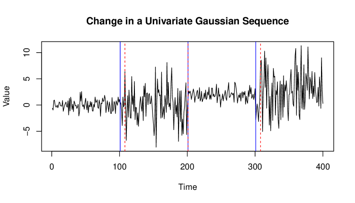
R> ts.plot(Xnorm,ylab=’Value’,main=’Change in a Univariate Gaussian Sequence’)R> abline(v=c(101,201,301),col=’blue’)R> abline(v=output1$estimates[c(-1,-5)],col=’red’,lty=2) As can be seen, if $\alpha=2$ the E-Divisive method can only identify changes in mean. For this reason, it is recommended that $\alpha$ is selected so as to lie in the interval $(0,2)$, in general. Figure 1 depicts the example time series, along with the estimated change points from the E-Divisive method when using $\alpha=1$.

Furthermore, when applying the E-Agglo method to this same simulated dataset, we obtain similar results. In the R code below we present the case for $\alpha=1$.

R> library("ecp")R> member <- rep(1:40,rep(10,40))R> output <- e.agglo(X = Xnorm, member = member, alpha = 1)R> output$opt

[1]   1 101 201 301 401

R> tail(output$fit,5)

[1] 100.05695 107.82542 104.30608 102.64330 -17.10722

R> output$progression[1,1:10]

[1]  1 11 21 31 41 51 61 71 81 91

R> output$merged[1:4,]

     [,1] [,2][1,]  -39  -40[2,]   -1   -2[3,]  -38    1[4,]    2   -3

Figure 1: Simulated independent Gaussian observations with changes in mean or variance. Dashed vertical lines indicate the change point locations estimated by the E-Divisive method, when using $\alpha=1$. Solid vertical lines indicate the true change point locations.

5.2 Multivariate change in covariance

To demonstrate that our methods do not just identify changes in marginal distributions we consider a multivariate example with only a change in covariance. In this example the marginal distributions remain the same, but the joint distribution changes. Therefore, applying a univariate change point procedure to each margin, such as those implemented by the chagenpoint, cmp, and bcp packages, will not detect the changes. The observations in this example are drawn from trivariate normal distributions with mean vector $\mu=(0,0,0)^{\top}$ and the following covariance matrices:

$$\begin{pmatrix}1&0&0\\ 0&1&0\\ 0&0&1\end{pmatrix},\begin{pmatrix}1&0.9&0.9\\ 0.9&1&0.9\\ 0.9&0.9&1\end{pmatrix},\mbox{ and}\begin{pmatrix}1&0&0\\ 0&1&0\\ 0&0&1\end{pmatrix}.$$

Observations are generated by using the mvtnorm package (Genz et al., 2012).

R> set.seed(200)R> library("ecp")R> library("mvtnorm")R> mu <- rep(0,3)R> covA <- matrix(c(1,0,0,0,1,0,0,0,1),3,3)R> covB <- matrix(c(1,0.9,0.9,0.9,1,0.9,0.9,0.9,1),3,3)R> period1 <- rmvnorm(250, mu, covA)R> period2 <- rmvnorm(250, mu, covB)R> period3 <- rmvnorm(250, mu, covA)R> Xcov <- rbind(period1, period2, period3)R> DivOutput <- e.divisive(Xcov, R = 499, alpha = 1)R> DivOutput$estimates

[1]   1 250 502 751

R> member <- rep(1:15,rep(50,15))R> pen = function(x){-length(x)}R> AggOutput1 <- e.agglo(X = Xcov, member = member, alpha = 1)R> AggOutput2 <- e.agglo(X = Xcov, member = member, alpha = 1, penalty = pen)R> AggOutput1$opt

[1] 1 101 201 301 351 501 601 701 751

R> AggOutput2$opt

[1] 301 501 In this case, the default procedure generates too many change points, as can be seen by the result of AggOutput1. When penalizing based upon the number of change points we obtain a much more accurate result, as shown by AggOutput2. Here the E-Agglo method has indicated that observations 1 through 300 and observations 501 through 750 are identically distributed.

5.3 Multivariate change in tails

For our second multivariate example we consider the case where the change in distribution is caused by a change in tail behavior. Data points are drawn from a bivariate normal distribution and a bivariate t-distribution with 2 degrees of freedom. Figure 2 depicts the different samples within the time series.

R> set.seed(100)R> library("ecp")R> library("mvtnorm")R> mu <- rep(0,2)R> period1 <- rmvnorm(250, mu, diag(2))R> period2 <- rmvt(250, sigma = diag(2), df = 2)R> period3 <- rmvnorm(250, mu, diag(2))R> Xtail <- rbind(period1, period2, period3)R> output <- e.divisive(Xtail, R = 499, alpha = 1)R> output$estimates

[1]   1 257 504 751

Figure 2: Data set used for the change in tail behavior example from Section 5.3. Periods 1 and 3 contain independent bivariate Gaussian observations with mean vector $(0,0)^{\top}$ and identity covariance matrix. The second time period contains independent observations from a bivariate Student’s t-distribution with 2 degrees of freedom and identity covariance matrix.

5.4 Inhomogeneous spatio-temporal point process

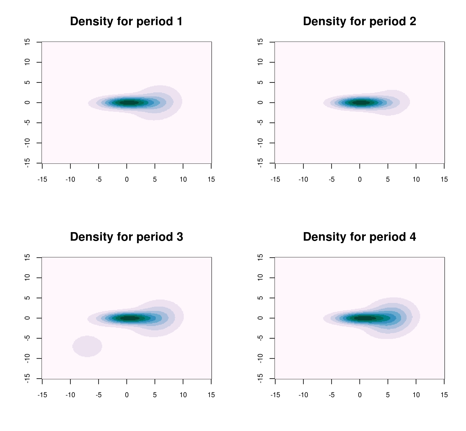
We apply the E-Agglo procedure to a spatio-temporal point process. The examined dataset consist of 10,498 observations, each with associated time and spatial coordinates. This dataset spans the time interval $[0,7]$ and has spatial domain $\mathbb{R}^{2}$. It contains 3 change points, which occur at times $t_{1}=1,t_{2}=3,$ and $t_{3}=4.5$. Over each of these subintervals, $t\in[t_{i},t_{i+1}]$ the process is an inhomogeneous Poisson point process with intensity function $\lambda(s,t)=f_{i}(s)$, a 2-d density function, for $i=1,2,3,4$. This intensity function is chosen to be the density function from a mixture of 3 bivariate normal distributions,

$${\mathcal{N}}\left(\begin{pmatrix}-7\\ -7\end{pmatrix},\begin{pmatrix}25&0\\ 0&25\end{pmatrix}\right),\ \ {\mathcal{N}}\left(\begin{pmatrix}0\\ 0\end{pmatrix},\begin{pmatrix}9&0\\ 0&1\end{pmatrix}\right),\ \mbox{and}\ \ {\mathcal{N}}\left(\begin{pmatrix}5.5\\ 0\end{pmatrix},\begin{pmatrix}9&0.9\\ 0.9&9\end{pmatrix}\right).$$

For the time periods, $[0,1],(1,3],(3,4.5],$ and $(4.5,7]$ the respective mixture weights are

$$\left(\frac{1}{3},\frac{1}{3},\frac{1}{3}\right),\ \left(\frac{1}{5},\frac{1}{2},\frac{3}{10}\right),\ \left(\frac{7}{20},\frac{3}{10},\frac{7}{20}\right),\ \mbox{and}\ \left(\frac{1}{5},\frac{3}{10},\frac{1}{2}\right).$$

To apply the E-Agglo procedure we initially segment the observations into 50 segments such that each segment spans an equal amount of time. At its termination, the E-Agglo procedure, with no penalty, identified change points at times 0.998, 3.000, and 4.499. These results can be obtained with the following

R> library("mvtnorm"); library("combinat"); library("MASS"); library("ecp")R> set.seed(2013)R>R> lambda <- 1500  # This is the overall arrival rate per unit time.R> #set of distribution meansR> muA <- c(-7,-7); muB <- c(0,0); muC <- c(5.5,0)R> #set of distribution covariance matricesR> covA <- 25*diag(2)R> covB <- matrix(c(9,0,0,1),2)R> covC <- matrix(c(9,.9,.9,9),2)R> #time intervalsR> time.interval <- matrix(c(0,1,3,4.5,1,3,4.5,7),4,2)R> #mixing coefficentsR> mixing.coef <- rbind(c(1/3,1/3,1/3),c(.2,.5,.3),c(.35,.3,.35),c(.2,.3,.5))R>R> stppData <- NULLR> for(i in 1:4){+  count <- rpois(1, lambda* diff(time.interval[i,]))+  Z <- rmultz2(n = count, p = mixing.coef[i,])+  S <- rbind(rmvnorm(Z[1],muA,covA), rmvnorm(Z[2],muB,covB),+    rmvnorm(Z[3],muC,covC))+  X <- cbind(rep(i,count), runif(n = count, time.interval[i,1],+    time.interval[i,2]), S)+  stppData <- rbind(stppData, X[order(X[,2]),])+ }R>R> member <- as.numeric(cut(stppData[,2], breaks = seq(0,7,by=1/12)))R> output <- e.agglo(X = stppData[,3:4], member = member, alpha = 1) The E-Agglo procedure was also run on the above data set using the following penalty function,

• pen <- function(cp){ -length(cp) }

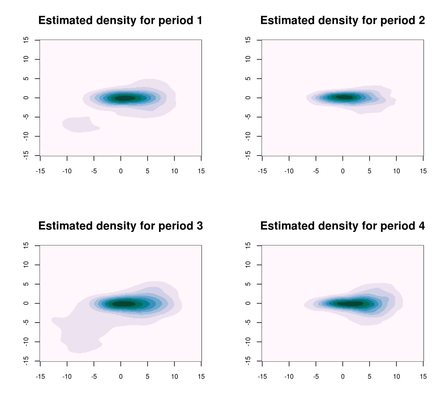
When using pen, change points were also estimated at times 0.998, 3.000, 4.499 The progression of the goodness-of-fit statistic for the different schemes is plotted in Figure 3. A comparison of the true densities and the estimated densities obtained from the procedure’s results with no penalty are shown in Figures 4 and  5, respectively. As can be see, the estimated results obtained from the E-Agglo procedure provide a reasonable approximation to the true densities.

Figure 3: The progression of the goodness-of-fit statistic for the various penalization schemes discussed in Section 5.4.

Figure 4: True density plots for the different segments of the spatio-temporal point process in Section 5.4.

Figure 5: Estimated density plots for the estimated segmentation provided by the E-Agglo procedure when applied to the spatio-temporal point process in Section 5.4.

6 Real data

In this section we analyze the results obtained by applying the E-Divisive and E-Agglo methods to two real datasets. We first apply our procedures to the micro-array aCGH data from Bleakley and Vert (2011). In this dataset we are provided with records of the copy-number variations for multiple individuals. Next we examine a set of financial time series. For this we consider weekly log returns of the companies which compose the Dow Jones Industrial Average.

6.0.1 Micro-array data

This dataset consists of micro-array data for 57 different individuals with a bladder tumor. Since all individuals have the same disease, we would expect the change point locations to be almost identical on each micro-array set. In this setting, a change point would correspond to a change in copy-number, which is assumed to be constant within each segment. The Group Fused Lasso (GFL) approach taken by Bleakley and Vert (2011) is well suited for this task since it is designed to detect changes in mean. We compare the results of our E-Divisive and E-Agglo approaches, when using $\alpha=2$, to those obtained by the GFL. In addition, we also consider another nonparametric change point procedure which is able to detect changes in both mean and variability, called MultiRank (Lung-Yut-Fong et al., 2011).

The original dataset from Bleakley and Vert (2011) contained missing values, and thus our procedure could not be directly applied. Therefore, we removed all individuals for which more than 7% of the values were missing. The remaining missing values we replaced by the average of their neighboring values. After performing this cleaning process, we were left with a sample of $d=43$ individuals and size $T=2215$. This dataset can be obtained through the following R commands;

R> library("ecp")R> data("ACGH")R> acghData = ACGH$data When applied to the full 43 dimensional series, the GFL procedure estimated 14 change points and the MultiRank procedure estimated 43. When using $\alpha=2,$ the E-Divisive procedure estimated 86 change points and the E-Agglo estimated 28.

Figures 6 and 7 provide the results of applying the various methods to a subsample of two individuals (persons 10 and 15). The E-Divisive procedure was run with min.size=15, and R=499, and the initial segmentation provided to the E-Agglo method consisted of equally sized segmens of length 15. The marginal series are plotted, and the dashed lines are the estimated change point locations.

Figure 6: The aCGH data for individual 10. Estimated change point locations are indicated by dashed vertical lines.

Figure 7: The aCGH data for individual 15. Estimated change point locations are indicated by dashed vertical lines.

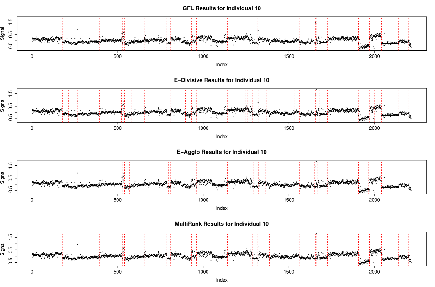
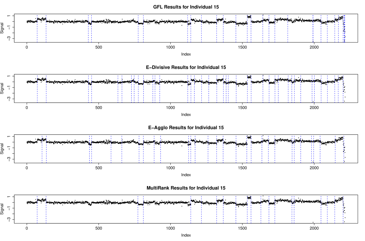
Looking at the returned estimated change point locations for the full 43-dimensional series we notice that both the E-Divisive and E-Agglo methods identified all of the change points returned by the GFL procedure. Further examination also shows that in addition to those change points found by the GFL procedure, the E-Divisive procedure also identified changes in the means of the marginal series. However, if we examine the first 14 to 20 change points estimated by the E-Divisive procedure we observe that they are those obtained by the GFL approach. This phenomenon however, does not appear when looking at the results from the E-Agglo procedure. Intuitively this is due to the fact that we must provide an initial segmentation of the series, which places stronger limitations on possible change point locaitons, than does specifying a minimum segment size.

6.0.2 Financial data

Next we consider weekly log returns for the companies which compose the Dow Jones Industrial Average (DJIA). The time period under consideration is April 1990 to January 2012, thus providing us with $T=1139$ observations. Since the time series for Kraft Foods Inc. does not span this entire period, it is not included in our analysis. This dataset is accessible by running data("DJIA").

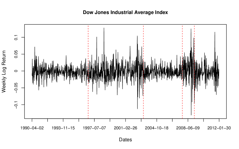
When applied to the 29 dimensional series, the E-Divisive method identified change points at 7/13/98, 3/24/03, 9/15/08, and 5/11/09. The change points at 5/11/09 and 9/15/08 correspond to the release of the Supervisory Capital Asset Management program results, and the Lehman Brothers bankruptcy filing, respectively. If we initially segment the dataset into segments of length 30 and apply the E-Agglo procedure, we identify change points at 1/3/00, 11/18/02, 8/18/08, and 3/16/09. The change points at 1/3/00 and 3/16/09 correspond to the passing of the Gramm-Leach-Bliley Act and the American Recovery and Reinvestment Act respectively.

For comparison we also considered the univariate time series for the DJIA Index weekly log returns. In this setting, the E-Divisive method identified change points at 10/21/96, 3/31/03, 10/15/07, and 3/9/09. While the E-Agglo method identified change points at 8/18/08 and 3/16/09. Once again, some of these change points correspond to major financial events. The change point at 3/9/09 correspond to Moody’s rating agency threatening to downgrade Wells Fargo & Co., JP Morgan Chase & Co., and Bank of America Corp. The 10/15/07 change point is located around the time of the financial meltdown caused by subprime mortgages. In both the univariate and multivariate cases the change point in March 2003 is around the time of the 2003 U.S. invasion of Iraq. A plot of the DJIA weekly log returns is provided in Figure 8 along with the locations of the estimated change points by the E-Divisive method.

For the E-Divisive method, the set of change points obtained from the univariate and multivariate analysis closely correspond to the same events. However, in the case of the E-Agglo method, the multivariate analysis is able to identify significant events that were not able to be detected from the univariate series. For this reason, we would argue that regardless of the method being used, it is recommended that multivariate analysis be performed.

Figure 8: Weekly log returns for the Dow Jones Industrial Average index from April 1990 to January 2012. The dashed vertical lines indicate the locations of estimated change points. The estimated change points are located at 10/21/96, 3/31/03, 10/15/07, and 3/9/09.

7 Performance analysis

To compare the performance of different change point methods we used the Rand Index (Rand, 1971) as well as Morey and Agresti’s Adjusted Rand Index (Morey and Agresti, 1984). These indices provide a measure of similarity between two different segmentations of the same set of observations.

The Rand Index evaluates similarity by examining the segment membership of pairs of observations. A shortcoming of the Rand Index is that it does not measure departure from a given baseline model, thus making it difficult to compare two different estimated segmentations. The hypergeometric model is a popular choice for the baseline, and is used by Hubert and Arabie (1985) and Fowlkes and Mallows (1983).

In our simulation study the Rand and Adjusted Rand Indices are determined by comparing the segmentation created by a change point procedure and the true segmentation. We compare the performance of our E-Divisive procedure against that of our E-Agglo. The results of the simulations are provided in Tables 1, 2 and 3. Tables 1 and 2 provide the results for simulations with univariate time series, while Table 3 provides the results for the multivariate time series. In these tables, average Rand Index along with standard errors are reported for 1000 simulations. Although not reported, similar results are obtained for the average Adjusted Rand Index.

Both the Rand Index and Adjusted Rand Index can be easily obtained through the use of the adjustedRand function in the clues package (Chang et al., 2010). If U and V are membership vectors for two different segmentations of the data, then the required index values are obtained as follows,

R> library(clues)R> RAND <- adjustedRand(U,V) The Rand Index is stored in RAND[1], while RAND[2] and RAND[3] store various Adjusted Rand indices. These Adjusted Rand indices make different assumptions on the baseline model, and thus arrive at different values for the expected Rand index.

	Change in Mean			Change in Variance
$T$	$\mu$	E-Divisive	E-Agglo	$\sigma^{2}$	E-Divisive	E-Agglo
150	1	$0.950_{0.001}$	$0.964_{0.004}$	2	$0.907_{0.003}$	$0.914_{0.012}$
	2	$0.992_{4.6\times 10^{-4}}$	$0.991_{0.001}$	5	$0.973_{0.001}$	$0.961_{0.002}$
	4	$1.000_{3.7\times 10^{-5}}$	$1.000_{0.000}$	10	$0.987_{7.1\times 10^{-4}}$	$0.978_{0.002}$
300	1	$0.972_{9.1\times 10^{-4}}$	$0.953_{0.002}$	2	$0.929_{0.003}$	$0.948_{0.021}$
	2	$0.996_{2.2\times 10^{-4}}$	$0.994_{6.4\times 10^{-4}}$	5	$0.990_{5.1\times 10^{-4}}$	$0.976_{0.001}$
	4	$1.000_{1.0\times 10^{-5}}$	$1.000_{0.000}$	10	$0.994_{3.2\times 10^{-4}}$	$0.988_{8.9\times 10^{-4}}$
600	1	$0.987_{1.5\times 10^{-5}}$	$0.970_{0.001}$	2	$0.968_{0.001}$	$0.551_{2.3\times 10^{-4}}$
	2	$0.998_{3.9\times 10^{-6}}$	$0.997_{3.0\times 10^{-4}}$	5	$0.995_{2.2\times 10^{-4}}$	$0.983_{8.7\times 10^{4}}$
	4	$1.000_{3.1\times 10^{-7}}$	$1.000_{0.000}$	10	$0.998_{1.5\times 10^{-4}}$	$0.992_{5.5\times 10^{-4}}$

Table 1: Average Rand Index and standard errors from 1,000 simulations for the E-Divisive and E-Agglo methods. Each sample has $T=150,300\;\mathrm{or}\;600$ observations, consisting of three equally sized clusters, with distributions $N(0,1),G,N(0,1)$, respectively. For changes in mean $G\equiv N(\mu,1)$, with $\mu=1,2,$ and $4$; for changes in variance $G\equiv N(0,\sigma^{2})$, with $\sigma^{2}=2,5,$ and $10$.

	Change in Tail
$T$	$\nu$	E-Divisive	E-Agglo
150	16	$0.835_{0.017}$	$0.544_{6.1\times 10^{-4}}$
	8	$0.836_{0.020}$	$0.543_{5.9\times 10^{-4}}$
	2	$0.841_{0.011}$	$0.545_{7.5\times 10^{-4}}$
300	16	$0.791_{0.015}$	$0.552_{2.1\times 10^{-4}}$
	8	$0.729_{0.018}$	$0.551_{2.2\times 10^{-4}}$
	2	$0.815_{0.006}$	$0.551_{2.3\times 10^{-4}}$
600	16	$0.735_{0.019}$	$0.552_{2.1\times 10^{-4}}$
	8	$0.743_{0.025}$	$0.551_{2.2\times 10^{-4}}$
	2	$0.817_{0.006}$	$0.552_{2.3\times 10^{-4}}$

Table 2: Average Rand Index and standard errors from 1,000 simulations for the E-Divisive and E-Agglo methods. Each sample has $T=150,300\;\mathrm{or}\;600$ observations, consisting of three equally sized clusters, with distributions $N(0,1),G,N(0,1)$, respectively. For the changes in tail shape $G\equiv t_{\nu}(0,1)$, with $\nu=16,8,$ and $2$.

	Change in Mean			Change in Correlation
$T$	$\mu$	E-Divisive	E-Agglo	$\rho$	E-Divisive	E-Agglo
300	1	$0.987_{4.7\times 10^{-4}}$	$0.978_{0.001}$	0.5	$0.712_{0.018}$	$0.551_{2.5\times 10^{-4}}$
	2	$0.992_{8.9\times 10^{-5}}$	$0.999_{2.4\times 10^{4}}$	0.7	$0.758_{0.021}$	$0.552_{2.4\times 10^{-4}}$
	3	$1.000_{1.3\times 10^{-5}}$	$1.000_{0.000}$	0.9	$0.769_{0.017}$	$0.550_{3.1\times 10^{-4}}$
600	1	$0.994_{2.2\times 10^{-4}}$	$0.986_{8.6\times 10^{4}}$	0.5	$0.652_{0.022}$	$0.553_{1.4\times 10^{-4}}$
	2	$1.000_{4.3\times 10^{-5}}$	$0.999_{1.5\times 10^{-4}}$	0.7	$0.650_{0.017}$	$0.553_{1.5\times 10^{-4}}$
	3	$1.000_{3.3\times 10^{-6}}$	$1.000_{0.000}$	0.9	$0.806_{0.019}$	$0.553_{1.8\times 10^{-4}}$
900	1	$0.996_{1.6\times 10^{-4}}$	$0.991_{6.0\times 10^{-4}}$	0.5	$0.658_{0.024}$	$0.554_{9.9\times 10^{-5}}$
	2	$1.000_{3.0\times 10^{-5}}$	$1.000_{7.3\times 10^{-5}}$	0.7	$0.633_{0.022}$	$0.554_{1.1\times 10^{-4}}$
	3	$1.000_{5.2\times 10^{-6}}$	$1.000_{2.2\times 10^{-5}}$	0.9	$0.958_{0.004}$	$0.553_{1.3\times 10^{-4}}$

Table 3: Average Rand Index and standard errors from 1,000 simulations for the E-Divisive and E-Agglo methods, when applied to multivariate time series with $d=2$. Each sample has $T=150,300\;\mathrm{or}\;600$ observations, consisting of three equally sized clusters, with distributions $N_{2}(0,I),G,N_{2}(0,I)$, respectively. For changes in mean $G\equiv N_{2}(\mu,I)$, with $\mu=(1,1)^{\top},(2,2)^{\top},$ and $(3,3)^{\top}$; for changes in correlation $G\equiv N(0,\Sigma_{\rho})$, in which the diagonal elements of $\Sigma_{\rho}$ are $1$ and the off-diagonal are $\rho$, with $\rho=0.5,0.7,$ and $0.9$.

8 Conclusion

The ecp package is able to perform nonparametric change point analysis of multivariate data. The package provides two primary methods for performing analysis, each of which is able to determine the number of change points without user input. The only necessary user-provided parameter, apart from the data itself, is the choice of $\alpha$. If $\alpha$ is selected to lie in the interval $(0,2),$ then the methods provided by this package are able to detect any type of distributional change within the observed series, provided that the absolute $\alpha$th moments exists.

The E-Divisive method sequentially tests the statistical significance of each change point estimate given the previously estimated change locations, while the E-Agglo method proceeds by optimizing a goodness-of-fit statistic. For this reason, we prefer to use the E-Divisive method, even though its running time is output-sensitive and depends on the number of estimated change points.

Through the provided examples, applications to real data, and simulations (Matteson and James, 2013), we observe that the E-Divisive approach obtains reasonable estimates for the locations of change points. Currently both the E-Divisive and E-Agglo methods have running times that are quadratic relative to the size of the time series. Future version of this package will attempt to reduce this to a linear relationship, or provide methods that can be used to quickly provide approximations.

Appendix A Appendix

This appendix provides additional details about the implementation of both the E-Divisive and E-Agglo methods in the ecp package.

A.1 Divisive outline

The E-Divisive method estimates change points with a bisection approach. In Algorithms 1 and  2, segment $C_{i}$ contains all observations in time interval $[\ell_{i},r_{i})$. Algorithm 2 demonstrates the procedure used to identify a single change point. The computational time to maximize over $(\tau,\kappa)$ is reduced to ${\mathcal{O}}(T^{2})$ by using memoization. Memoization also allows Algorithm 2 to execute its for loop at most twice. The permutation test is outlined by Algorithm 3. When given the segmentation $C$, a permutation is only allowed to reorder observations so that they remain within their original segments.

Inputs : Time series $Z$, significance level $p_{0}$, minimum segment size $m$, the maximum number of permutations for the permutation test $R$, the uniform resampling error bound $eps$, epsilon spending rate $h$, and $\alpha\in(0,2]$.

Output : A segmentation of the time series.

Create distance matrix $Z_{ij}^{\alpha}=|Z_{i}-Z_{j}|^{\alpha}$;

while Have not found a statisticaly insignificant change point 

       Estimate next most likely change point location;

       Test estimated change point for statistical significance;

       if Change point is statistically significant then

             Update the segmentation;

            

       end if

      

endwhile

return Final segmentation

Algorithm 1 Outline of the divisive procedure.

Inputs : Segmentation $C$, distance matrix $D$, minimum segment size m.

Output : A triple $(x,y,z)$ containing the following information: a segment identifier, a distance within a segment, a weighed sample divergence.

best = $-\infty$;

loc = 0;

for Segments $C_{i}\in C$ 

       $A$ = Within distance for $[\ell_{i},\ell_{i}+m)$;

       for $\kappa\in\{\ell_{i}+m+2,\dots,r_{i}+1\}$ 

             Calculate and store between and within distances for currenct choice of $\kappa$;

             Calculate test statistic;

             if Test statistic $\geq$ best then

                   Update best;

                   Update loc to m;

                  

             end if

            

       endfor

      for $\tau\in\{\ell_{i}+m+1,\dots,r_{i}-m\}$ 

             Update within distance for left segment;

             for $\kappa\in\{\tau+m+1,\dots,r_{i}+1\}$ 

                   Update remaining between and within distances for current choice of $\kappa$;

                   Calcualte test statistic;

                   if Test statistic $\geq$ best then

                         Update best;

                         Update loc to $\tau$;

                        

                   end if

                  

             endfor

            

       endfor

      

endfor

return Which segment to divide, loc, and best

Algorithm 2 Outline of procedure to locate a single change point.

Inputs : Distance matrix $D$, observed test statistic $\nu$, maximum number of permutations $R$, uniform resampling error bound $eps$, epsilon spending rate $h$, segmentation $C$, minimum segment size m.

Output : An approximate $p$ value.

over = 1;

for $i\in\{1,2,\dots,R\}$ 

       Permute rows and columns of $D$ based on the segmentation $C$ to create $D^{\prime}$;

       Obtain test statistic for permuted observations;

       if Permuted test statistic $\geq$ observed test statistic then

             over = over + 1;

            

       end if

      if An early termination condition is satisfied then

             return over/(i+1)

       end if

      

endfor

return over/(R+1)

Algorithm 3 Outline of the permutation test.

A.2 Agglomerative outline

The E-Agglo method estimates change point by maximizing the goodness-of-fit statistic given by Equation 2. The method must be provided an initial segmentation of the series. Segments are then merged in order to maximize the goodness-of-fit statistic. As segments are merged, their between-within distances also need to be updated. The following result due to Székely and Rizzo (2005) greatly reduces the computational time necessary to perform these updates.

Lemma 3.

Suppose that $C_{1},C_{2},$ and $C_{3}$ are disjoint segments with respective sizes $m_{1},m_{2},$ and $m_{3}$. Then if $C_{1}$ and $C_{2}$ are merged to form the segment $C_{1}\cup C_{2}$,

$$\widehat{\cal E}(C_{1}\cup C_{2},C_{3};\alpha)=\frac{m_{1}+m_{3}}{m_{1}+m_{2}+m_{3}}\widehat{\cal E}(C_{1},C_{3};\alpha)+\frac{m_{2}+m_{3}}{m_{1}+m_{2}+m_{3}}\widehat{\cal E}(C_{2},C_{3};\alpha)-\frac{m_{3}}{m_{1}+m_{2}+m_{3}}\widehat{\cal E}(C_{1},C_{2};\alpha).$$

Algorithm 4 is an outline for the agglomerative procedure. In this outline $C_{i+k}\ (C_{i-k})$ is the segment that is $k$ segments to the right (left) of $C_{i}$.

Inputs : An initial segmentation C, a time series $Z$, a penalty function $f(\vec{\tau})$, and $\alpha\in(0,2]$.

Output : A segmentation of the time series.

Create distance matrix $D_{i,j}=\widehat{\mathcal{E}}(C_{i},C_{j};\alpha)$;

Obtain initial penalized goodness-of-fit (gof) statistic;

for $K\in\{N,N+1,\dots,2N-3\}$ 

       Merge best candidate segments;

       Update current gof;

       if Current gof $\geq$ largest gof so far then

             Update largest gof

       end if

      

endfor

Penalize the sequence of obtained gof statistics;

Choose best segmentation based on penalized gof statistics;

return Best segmentation

Algorithm 4 Outline of the agglomerative procedure.

References

- Akoglu and Faloutsos (2010) Akoglu L, Faloutsos C (2010). “Event Detection in Time Series of Mobile Communication Graphs.” In Proc. of Army Science Conference. 2010 Army Science Conference.
- Bleakley and Vert (2011) Bleakley K, Vert JP (2011). “The Group Fused Lasso for Multiple Change-Point Detection.” Technical Report HAL-00602121, Bioinformatics Center (CBIO).
- Bolton and Hand (2002) Bolton R, Hand D (2002). “Statistical Fraud Detection: A Review.” Statistical Science, 17, 235 – 255.
- Chang et al. (2010) Chang F, Qiu W, Zamar RH, Lazarus R, Wang X (2010). “clues: An R Package for Nonparametric Clustering Based on Local Shrinking.” Journal of Statistical Software, 33(4), 1–16.
- Chasalow (2012) Chasalow S (2012). combinat: Combinatorics Utilities. R package version 0.0-8, URL http://CRAN.R-project.org/package=combinat.
- Erdman and Emerson (2007) Erdman C, Emerson JW (2007). “bcp: An R package for performing a Bayesian analysis of change point problems.” Journal of Statistical Software, 23(3), 1–13.
- Fowlkes and Mallows (1983) Fowlkes EB, Mallows CL (1983). “A Method for Comparing Two Hierarchical Clusterings.” Journal of the American Statistical Association, 78(383), 553 – 569.
- Gandy (2009) Gandy A (2009). “Sequential Implementation of Monte Carlo Tests With Uniformly Bounded Resampling Risk.” Journal of the American Statistical Association, 104(488), 1504–1511.
- Genz et al. (2012) Genz A, Bretz F, Miwa T, Mi X, Leisch F, Scheipl F, Hothorn T (2012). mvtnorm: Multivariate Normal and T Distributions.
- Gretton et al. (2007) Gretton A, Borgwardt K, Rasch M, Schölkopf B, Smola A (2007). “A Kernel Method for the Two Sample Problem.” In Advances in Neural Information Processing Systems 19, pp. 513–520. MIT Press.
- Hoeffding (1961) Hoeffding W (1961). “The Strong Law of Large Numbers for U-Statistics.” Technical Report 302, North Carolina State University. Dept. of Statistics.
- Hubert and Arabie (1985) Hubert L, Arabie P (1985). “Comparing Partitions.” Journal of Classification, 2(1), 193 – 218.
- Killick and Eckley (2011) Killick R, Eckley IA (2011). “changepoint: An R Package for Changepoint Analysis.”
- Killick et al. (2012) Killick R, Fearnhead P, Eckley I (2012). “Optimal Detection of Changepoints With a Linear Computational Cost.” Journal of the American Statistical Association, 107(500), 1590–1598.
- Lung-Yut-Fong et al. (2011) Lung-Yut-Fong A, Lévy-Leduc C, Cappé O (2011). “Homogeneity and Change-Point Detection Tests for Multivariate Data Using Rank Statistics.” ArXiv e-prints. 1107.1971.
- Mampaey and Vreeken (2011) Mampaey M, Vreeken J (2011). “Summarizing Categorical Data by Clustering Attributes.” Data Mining and Knowledge Discovery, 24, 1 – 44.
- Matteson and James (2013) Matteson DS, James NA (2013). “A Nonparametric Approach for Multiple Change Point Analysis of Multivariate Data.” ArXiv e-prints. To appear in the Journal of the American Statistical Association, 1306.4933.
- Morey and Agresti (1984) Morey LC, Agresti A (1984). “The Measurement of Classification Agreement: An Adjustment to the Rand Statistic for Chance Agreement.” Educational and Psychological Measurement, 44, 33 – 37.
- Muggeo and Adelfio (2011) Muggeo VM, Adelfio G (2011). “Efficient Change Point Detection for Genomic Sequences of Continuous Measurements.” Bioinformatics, 27, 161 – 166.
- R Development Core Team (2012) R Development Core Team (2012). R: A Language and Environment for Statistical Computing. R Foundation for Statistical Computing, Vienna, Austria. URL http://www.R-project.org/.
- Rand (1971) Rand WM (1971). “Objective Criteria for the Evaluation of Clustering Methods.” Journal of the American Statistical Association, 66, 846 – 850.
- Ross (2012) Ross GJ (2012). cpm: Sequential Parametric and Nonparametric Change Detection. R package version 1.0.
- Schauer et al. (2010) Schauer K, Duong T, Bleakley K, Bardin S, Bornens M, Goud B (2010). “Probabilistic Density Maps to Study Global Endomembrane Organization.” Nature Methods, 7(7), 560–566.
- Sequeira and Zaki (2002) Sequeira K, Zaki M (2002). “ADMIT: Anomaly-Based Data Mining for Intrusions.” In Proceedings of the Eighth ACM SIGKDD International Conference on Knowledge Discovery and Data Mining, KDD ’02. ACM.
- Székely and Rizzo (2005) Székely GJ, Rizzo ML (2005). “Hierarchical Clustering Via Joint Between-Within Distances: Extending Ward’s Minimum Variance Method.” Journal of Classification, 22(2), 151 – 183.
- Székely and Rizzo (2010) Székely GJ, Rizzo ML (2010). “Disco Analysis: A Nonparametric Extension of Analysis of Variance.” The Annals of Applied Statistics, 4(2), 1034–1055.
- Talih and Hengartner (2005) Talih M, Hengartner N (2005). “Structural Learning With Time-Varying Components: Tracking the Cross-Section of Financial Time Series.” Journal of the Royal Statistical Society, 67, 321 – 341.
- Venables and Ripley (2002) Venables WN, Ripley BD (2002). Modern Applied Statistics with S. Fourth edition. Springer-Verlag, New York. URL http://www.stats.ox.ac.uk/pub/MASS4.
- Zeileis et al. (2003) Zeileis A, Kleiber C, Krämer W, Hornik K (2003). “Testing and Dating of Structural Changes in Practice.” Computational Statistics & Data Analysis, 44, 109–123.
- Zeileis et al. (2002) Zeileis A, Leisch F, Hornik K, Kleiber C (2002). “strucchange: An R Package for Testing for Structural Change in Linear Regression Models.” Journal of Statistical Software, 7(2), 1–38. URL http://www.jstatsoft.org/v07/i02/.