Homogeneity and change-point detection tests for multivariate data using rank statistics

Alexandre Lung-Yut-Fong, Céline Lévy-Leduc, Olivier Cappé
Abstract

Detecting and locating changes in highly multivariate data is a major concern in several current statistical applications. In this context, the first contribution of the paper is a novel non-parametric two-sample homogeneity test for multivariate data based on the well-known Wilcoxon rank statistic. The proposed two-sample homogeneity test statistic can be extended to deal with ordinal or censored data as well as to test for the homogeneity of more than two samples. We also provide a detailed analysis of the power of the proposed test statistic (in the two sample case) against asymptotic local shift alternatives. The second contribution of the paper concerns the use of the proposed test statistic to perform retrospective change-point detection. It is first shown that the approach is computationally feasible even when looking for a large number of change-points thanks to the use of dynamic programming. Computable asymptotic p𝑝p-values for the test are available in the case where a single potential change-point is to be detected. The proposed approach is particularly recommendable in situations where the correlations between the coordinates of the data are moderate, the marginal distributions are not well modelled by usual parametric assumptions (e.g., in the presence of outliers) and when faced with highly variable change patterns, for instance, if the potential changes only affect subsets of the coordinates of the data.

1 Introduction

Detection and location of distributional changes in data is a major statistical challenge that arises in many different contexts. This very general concern can be particularised to more specific tasks such as segmentation, novelty detection or significance tests. In this contribution, we focus on two types of problems: homogeneity testing, where the statistician is presented with pre-specified groupings of the data that are believed to be comparable, and change-point detection, in which a series –most often, a time series– is to be segmented into homogeneous contiguous regions. These two tasks are obviously related but the latter is more challenging as the appropriate groupings of the data are unknown, although one does have the strong prior assumption that homogeneous regions of the data are contiguous. Homogeneity testing and/or change-point detection are instrumental in applications that range from the surveillance of industrial processes (Basseville and Nikiforov, 1993), to computer security (Tartakovsky et al., 2006; Lévy-Leduc and Roueff, 2009), processing of audiovisual data (Désobry et al., 2005), financial and econometric modelling (Bai and Perron, 2003; Talih and Hengartner, 2005), health monitoring (Brodsky and Darkhovsky, 2000), or bioinformatics (Picard et al., 2005; Vert and Bleakley, 2010).

In light of the important available literature on change-point detection it is important to make two additional distinctions. First, in many cases the data to be analysed can be assumed to present some form of global reproducibility and to include several instances of actual changes. In this case, it seems reasonable to fit a model to the data to profit from the available statistical information regarding various relevant aspects of the problem such as the distribution of the data in the absence of change, the typical change-point patterns, etc. In such situations, very convincing results have been demonstrated using Bayesian approaches due to the existence of efficient computational methods to explore the posterior distribution, even when using very flexible models (Barry and Hartigan, 1992; Fearnhead, 2006). In contrast, in this contribution, we consider scenarios in which the data are either scarce or very variable or where potential changes occur somewhat infrequently. In this alternative context, the goal is to develop approaches that make as few assumptions as possible regarding the underlying distribution of the data or the nature of the changes and that do not rely on the observation of actual change patterns. The second important distinction is that many works in the time series literature consider the online change-point detection framework (Siegmund, 1985) in which the data have to be processed on-the-fly or with minimal delay using for instance the CUSUM algorithm initially proposed by Page (1954). In the following, we consider the opposite situation, sometimes referred to as retrospective analysis, in which all the data to be tested have been recorded and are available for analysis.

In this context, the first contribution of this work consists in novel homogeneity tests for dealing with possibly high-dimensional multivariate observations. We focus on situations where the potential changes are believed to have a strong impact on the mean but where the distribution of the data is otherwise mostly unknown. For scalar observations, there are well-known robust solutions for testing homogeneity in this context such as the Wilcoxon/Mann–Whitney or Kruskal-Wallis procedures (Lehmann, 1975) to be further discussed below. For multivariate observations, the situation is far more challenging as one would like to achieve robustness with respect both to the form of the marginal distributions and to the existence of correlations (or other form of dependence) between coordinates. The latter aspect has been addressed in a series of works by Möttönen et al. (1997); Hettmansperger et al. (1998); Oja (1999); Topchii et al. (2003) who studied multivariate extensions of sign and rank tests. These tests are affine invariant in the sense that they behave similarly to Hotelling’s T2superscript𝑇2T^{2} test (see Section 2.3 below) —which is optimal for Gaussian distributions– for general classes of multivariate distributions having ellipsoidal contours (e.g., for multivariate t𝑡t distributions). Another promising approach investigated by several recent works consists in using kernel-based methods (Désobry et al., 2005; Gretton et al., 2006; Harchaoui et al., 2008). In our experience however, these methods that can achieve impressive results for moderately multidimensional data or in specific situations (e.g., if the data lie on a low-dimensional manifold) lack robustness when moving to larger dimensions. In particular, as illustrated in Section 4.1 below, kernel-based methods are not robust with respect to the presence of contaminating noise and to the fact that the changes to be detected may only affect a subset of the components of the high-dimensional data. The latter scenario is of very important practical significance in applications where the data to be analysed consist in exhaustive recordings of complex situations that are only partly affected by possible changes (see Lévy-Leduc and Roueff (2009) for an example regarding the detection of computer attacks). The method proposed in this work is based on a combination of marginal rank statistics, following the pioneering idea of Wei and Lachin (1984). Compared to the latter, our contribution is twofold: first, we show how to correct the bias that appears in the test statistic proposed by Wei and Lachin (1984) whenever the two samples are not balanced in size; we then show how to extend this idea to the case of more than two groups. The numerical simulation presented in Section 4 confirms that the proposed test statistic is significantly more robust than kernel-based methods or approaches based on least-squares or Hotelling’s T2superscript𝑇2T^{2} statistics. These empirical observations are also supported by the results detailed in Section 2.3 regarding the power of the proposed test statistic (in the two sample case) with respect to asymptotic local shift alternatives. In particular, although the proposed test is not strictly affine invariant111It is highly unlikely that there exist statistics which are both invariant under monotonic transformations of the marginals –as the proposed method is– and affine invariant. it compares favourably to Hotelling’s T2superscript𝑇2T^{2} statistic for important classes of distributions under the assumption that the condition number of the correlation matrix of the data is not too large.

We then consider the use of the proposed approach for change-point detection by optimising the test statistic over the –now considered unknown– positions of the segment boundaries. Although simple this idea raises two type of difficulties. The first one is computational as the resulting optimisation task is combinatorial and cannot be solved by brute force enumeration when there is more than one change-point (that is, two segments). In the literature this issue has been previously tackled either using dynamic programming (Bai and Perron, 2003; Harchaoui and Cappé, 2007) or more recently using Lasso-type penalties (Harchaoui and Lévy-Leduc, 2010; Vert and Bleakley, 2010). We show that the generic dynamic programming strategy is applicable to the proposed test statistic making it practically suitable for retrospective detection of multiple change-points. The second difficulty is statistical as the optimisation with respect to the change-point locations modifies the distribution of the test statistics. Thus, the design of quantitative criterions for assessing the significance of the test is a challenging problem in this context. This issue has been considered before, mostly in the case of a single change-point, for various test statistics (Csörgő and Horváth, 1997; Chen and Gupta, 2000). In many cases the asymptotic distribution of the test remains hard to characterise and must be calibrated using Monte Carlo simulations. We show that for a simple modification of the proposed rank-based statistic, one can indeed obtain computable asymptotic p𝑝p-values that can be used to assess the significance of the test when looking for a single change-point.

The paper is organised as follows. Section 2 is devoted to homogeneity testing, starting first with the two-sample case and then considering the more general situation where several predefined groups are available. The end of Section 2 is dedicated to the study of the asymptotic behaviour of the two-sample homogeneity test under local shift alternatives. In Section 3, the proposed test statistic is modified to provide a method for detecting and locating change-points, with the computation of p𝑝p-values (in the single change-point case) being discussed in Section 3.2. The results of numerical experiments carried out both on simulated and on real data are then reported in Section 4.

2 Testing for Homogeneity

We first tackle in this Section the so-called two-sample problem, that is testing the homogeneity between two partitions of data. The proposed test statistic is then extended in Section 2.2 to deal with more than two groups of data.

2.1 Two-sample homogeneity test

Consider n𝑛n K𝐾K-dimensional multivariate observations (𝐗1,,𝐗n)subscript𝐗1subscript𝐗𝑛(\mathbf{X}_{1},\dots,\mathbf{X}_{n}) and denote by Xi,ksubscript𝑋𝑖𝑘X_{i,k} the k𝑘kth coordinate of Xisubscript𝑋𝑖X_{i}, such that 𝐗i=(Xi,1,,Xi,K)subscript𝐗𝑖superscriptsubscript𝑋𝑖1subscript𝑋𝑖𝐾\mathbf{X}_{i}=(X_{i,1},\dots,X_{i,K})^{\prime}, where the prime is used to denote transposition. We consider the classical statistic test framework with the null (or baseline) hypothesis, (H0)subscript𝐻0(H_{0}): “(𝐗1,,𝐗n)subscript𝐗1subscript𝐗𝑛(\mathbf{X}_{1},\dots,\mathbf{X}_{n}) are identically distributed random vectors”, and the alternative hypothesis, (H1)subscript𝐻1(H_{1}): “(𝐗1,,𝐗n1)subscript𝐗1subscript𝐗subscript𝑛1(\mathbf{X}_{1},\dots,\mathbf{X}_{n_{1}}) are distributed under 1subscript1\mathbb{P}_{1} and (𝐗n1+1,,𝐗n)subscript𝐗subscript𝑛11subscript𝐗𝑛(\mathbf{X}_{n_{1}+1},\dots,\mathbf{X}_{n}) under 2subscript2\mathbb{P}_{2}, with 12subscript1subscript2\mathbb{P}_{1}\neq\mathbb{P}_{2}”. In this setting, the potential change point n1subscript𝑛1n_{1} is assumed to be given but the data distributions are fully unspecified both under (H0)subscript𝐻0(H_{0}) and (H1)subscript𝐻1(H_{1}). The proposed test statistic extends the well-known Wilcoxon/Mann–Whitney rank-based criterion to multivariate data by considering the asymptotic joint behaviour of the rank statistics that can be computed from each coordinate of the observations. For k𝑘k in {1,,K}1𝐾\{1,\dots,K\}, define the vector-valued statistic 𝐔n(n1)=(Un,1(n1),,Un,K(n1))subscript𝐔𝑛subscript𝑛1superscriptsubscript𝑈𝑛1subscript𝑛1subscript𝑈𝑛𝐾subscript𝑛1\mathbf{U}_{n}(n_{1})=(U_{n,1}(n_{1}),\dotsc,U_{n,K}(n_{1}))^{\prime} by

Un,k(n1)=1nn1(nn1)i=1n1j=n1+1n{𝟏(Xi,kXj,k)𝟏(Xj,kXi,k)}.subscript𝑈𝑛𝑘subscript𝑛11𝑛subscript𝑛1𝑛subscript𝑛1superscriptsubscript𝑖1subscript𝑛1superscriptsubscript𝑗subscript𝑛11𝑛1subscript𝑋𝑖𝑘subscript𝑋𝑗𝑘1subscript𝑋𝑗𝑘subscript𝑋𝑖𝑘U_{n,k}(n_{1})=\frac{1}{\sqrt{nn_{1}(n-n_{1})}}\sum_{i=1}^{n_{1}}\sum_{j=n_{1}+1}^{n}\left\{\mathbf{1}(X_{i,k}\leq X_{j,k})-\mathbf{1}(X_{j,k}\leq X_{i,k})\right\}\;. (1)

Although the form of the statistic given above is more appropriate for mathematical analysis as well as for discussing possible generalisations of the approach (see Section 2.1.2 below), it is important to realise that Un,k(n1)subscript𝑈𝑛𝑘subscript𝑛1U_{n,k}(n_{1}) is related to the classical Wilcoxon/Mann–Whitney statistic computed from the series X1,k,,Xn,ksubscript𝑋1𝑘subscript𝑋𝑛𝑘X_{1,k},\dots,X_{n,k}. Assuming that there are no ties in the data, let Rj(k)superscriptsubscript𝑅𝑗𝑘R_{j}^{(k)} denote the rank of Xj,ksubscript𝑋𝑗𝑘X_{j,k} among (X1,k,,Xn,k)subscript𝑋1𝑘subscript𝑋𝑛𝑘(X_{1,k},\dots,X_{n,k}), that is, Rj(k)=i=1n𝟏(Xi,kXj,k)superscriptsubscript𝑅𝑗𝑘superscriptsubscript𝑖1𝑛1subscript𝑋𝑖𝑘subscript𝑋𝑗𝑘R_{j}^{(k)}=\sum_{i=1}^{n}\mathbf{1}(X_{i,k}\leq X_{j,k}). Noticing that j=1nRj(k)=n(n+1)/2superscriptsubscript𝑗1𝑛superscriptsubscript𝑅𝑗𝑘𝑛𝑛12\sum_{j=1}^{n}R_{j}^{(k)}=n(n+1)/2, it is then easily verified that Un,k(n1)subscript𝑈𝑛𝑘subscript𝑛1U_{n,k}(n_{1}) can be equivalently defined as

Un,k(n1)=2nn1(nn1)i=1n1(n+12Ri(k))=2nn1(nn1)j=n1+1n(Rj(k)n+12).subscript𝑈𝑛𝑘subscript𝑛12𝑛subscript𝑛1𝑛subscript𝑛1superscriptsubscript𝑖1subscript𝑛1𝑛12superscriptsubscript𝑅𝑖𝑘2𝑛subscript𝑛1𝑛subscript𝑛1superscriptsubscript𝑗subscript𝑛11𝑛superscriptsubscript𝑅𝑗𝑘𝑛12U_{n,k}(n_{1})=\frac{2}{\sqrt{nn_{1}(n-n_{1})}}\sum_{i=1}^{n_{1}}\left(\frac{n+1}{2}-R_{i}^{(k)}\right)=\frac{2}{\sqrt{nn_{1}(n-n_{1})}}\sum_{j=n_{1}+1}^{n}\left(R_{j}^{(k)}-\frac{n+1}{2}\right)\;. (2)

This alternative form of Un,k(n1)subscript𝑈𝑛𝑘subscript𝑛1U_{n,k}(n_{1}) is more appropriate for computational purposes as discussed in Section 2.1.1 below. For convenience, we denote by F^n,k(t)=n1j=1n𝟏(Xj,kt)subscript^𝐹𝑛𝑘𝑡superscript𝑛1superscriptsubscript𝑗1𝑛1subscript𝑋𝑗𝑘𝑡\hat{F}_{n,k}(t)=n^{-1}\sum_{j=1}^{n}\mathbf{1}(X_{j,k}\leq t) the empirical cumulative distribution function (c.d.f. in short) of the k𝑘kth coordinate, such that F^n,k(Xi,k)=Ri(k)/nsubscript^𝐹𝑛𝑘subscript𝑋𝑖𝑘superscriptsubscript𝑅𝑖𝑘𝑛\hat{F}_{n,k}(X_{i,k})=R_{i}^{(k)}/n. Let Σ^nsubscript^Σ𝑛\hat{\Sigma}_{n} denote the K𝐾K-dimensional empirical covariance matrix defined by

Σ^n,kk=4ni=1n{F^n,k(Xi,k)1/2}{F^n,k(Xi,k)1/2}, 1k,kK.formulae-sequencesubscript^Σ𝑛𝑘superscript𝑘4𝑛superscriptsubscript𝑖1𝑛subscript^𝐹𝑛𝑘subscript𝑋𝑖𝑘12subscript^𝐹𝑛superscript𝑘subscript𝑋𝑖superscript𝑘12formulae-sequence1𝑘superscript𝑘𝐾\hat{\Sigma}_{n,kk^{\prime}}=\frac{4}{n}\sum_{i=1}^{n}\{\hat{F}_{n,k}(X_{i,k})-1/2\}\{\hat{F}_{n,k^{\prime}}(X_{i,k^{\prime}})-1/2\},\;1\leq k,k^{\prime}\leq K\;. (3)

The test statistic that we propose for assessing the presence of a potential change in n1subscript𝑛1n_{1} is defined as

Sn(n1)=𝐔n(n1)Σ^n1𝐔n(n1).subscript𝑆𝑛subscript𝑛1subscript𝐔𝑛superscriptsubscript𝑛1superscriptsubscript^Σ𝑛1subscript𝐔𝑛subscript𝑛1S_{n}(n_{1})=\mathbf{U}_{n}(n_{1})^{\prime}\hat{\Sigma}_{n}^{-1}\mathbf{U}_{n}(n_{1})\;. (4)

Theorem 1 below (proved in Appendix A) gives the limiting behaviour of the test statistic Sn(n1)subscript𝑆𝑛subscript𝑛1S_{n}(n_{1}) under the null hypothesis.

Theorem 1

Let 𝐗1,,𝐗n1,𝐗n1+1,,𝐗nsubscript𝐗1subscript𝐗subscript𝑛1subscript𝐗subscript𝑛11subscript𝐗𝑛\mathbf{X}_{1},\dotsc,\mathbf{X}_{n_{1}},\mathbf{X}_{n_{1}+1},\dotsc,\mathbf{X}_{n} be Ksuperscript𝐾\mathbb{R}^{K}-valued i.i.d. random vectors, such that for all k𝑘k in {1,,K}1𝐾\{1,\dotsc,K\}, the cumulative distribution function Fksubscript𝐹𝑘F_{k} of X1,ksubscript𝑋1𝑘X_{1,k} is a continuous function. Assume that n1/nt1subscript𝑛1𝑛subscript𝑡1n_{1}/n\to t_{1} in (0,1) as n𝑛n tends to infinity, and that the K×K𝐾𝐾K\times K covariance matrix ΣΣ\Sigma defined by

Σkk=4Cov(Fk(X1,k);Fk(X1,k)), 1k,kK,formulae-sequencesubscriptΣ𝑘superscript𝑘4Covsubscript𝐹𝑘subscript𝑋1𝑘subscript𝐹superscript𝑘subscript𝑋1superscript𝑘formulae-sequence1𝑘superscript𝑘𝐾\Sigma_{kk^{\prime}}=4\operatorname*{Cov}\left(F_{k}(X_{1,k});F_{k^{\prime}}(X_{1,k^{\prime}})\right),\;1\leq k,k^{\prime}\leq K\;, (5)

is positive definite. Then, the test statistic Sn(n1)subscript𝑆𝑛subscript𝑛1S_{n}(n_{1}) defined in (4) converges in distribution to a χ2superscript𝜒2\chi^{2} distribution with K𝐾K degrees of freedom.

Theorem 1 shows that the proposed test is well normalised with respect to the dimension K𝐾K, the length n𝑛n of the data and the postulated change-point location n1subscript𝑛1n_{1}. It is asymptotically distribution-free in the sense that its limiting behaviour under (H0)subscript𝐻0(H_{0}) does not depend on the distribution of the data. By construction, it is also invariant under any monotonic transformation of the coordinates of 𝐗isubscript𝐗𝑖\mathbf{X}_{i}.

The matrix ΣΣ\Sigma, which corresponds to the asymptotic covariance matrix of the vector 𝐔n(n1)subscript𝐔𝑛subscript𝑛1\mathbf{U}_{n}(n_{1}) is equal, up to a multiplicative constant, to the Spearman correlation matrix of Xisubscript𝑋𝑖X_{i} (Lehmann, 1975; van der Vaart, 1998). This is a well-known robust measure of dependence that appears in particular when using copula models. A sufficient condition for ensuring the invertibility of ΣΣ\Sigma is thus that no linear combination of the Fk(X1,k)subscript𝐹𝑘subscript𝑋1𝑘F_{k}(X_{1,k})’s should be almost surely equal to a constant, which is arguably a very weak condition. It is easily checked that the diagonal elements of ΣΣ\Sigma are all equal to 1/3131/3 and that Σk=Σk=0subscriptΣ𝑘subscriptΣ𝑘0\Sigma_{k\ell}=\Sigma_{\ell k}=0 whenever the k𝑘k-th and \ell-th coordinates of 𝐗isubscript𝐗𝑖\mathbf{X}_{i} are independent. It appears, in practice, that the diagonal elements of Σ^nsubscript^Σ𝑛\hat{\Sigma}_{n} converge very rapidly to 1/3 value and we did not observe any significant improvement when trying to take into account this fact when estimating ΣΣ\Sigma.

Theorem 1 defines the asymptotic false alarm rate associated with the test statistic Sn(n1)subscript𝑆𝑛subscript𝑛1S_{n}(n_{1}). The test is consistent (i.e., its power tends to 1) for all alternatives such that the condition ensuring the consistency of the standard Wilcoxon/Mann–Whitney two-sample test holds true for at least one coordinate. More formally, the proposed test is consistent when there exists k𝑘k in {1,,K}1𝐾\{1,\dots,K\} such that (Xk,1Xk,n)1/2subscript𝑋𝑘1subscript𝑋𝑘𝑛12\mathbb{P}(X_{k,1}\leq X_{k,n})\neq 1/2. In the scalar case, this condition is known to hold for general classes of changes such as shift (change-in-the-mean) models or scale (multiplicative) change for positive variables. We defer to Section 3 a more detailed investigation of the asymptotic power of the test in the case of multivariate shift alternatives.

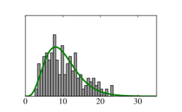
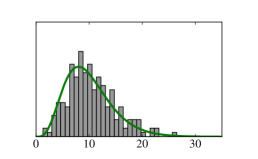
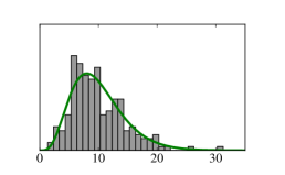
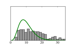
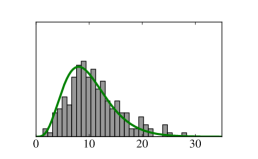
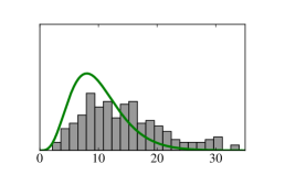
As Theorem 1 is an asymptotic result, we have carried out Monte Carlo simulations to asses the accuracy of the approximation for finite sample sizes. Using data with independent coordinates222Note that by construction, the test statistic is then fully invariant with respect to the precise distribution used for the Monte Carlo simulations. we found that the distribution of Sn(n1)subscript𝑆𝑛subscript𝑛1S_{n}(n_{1}) defined in (4) can be considered close enough to the limiting distribution, as measured by the Kolmogorov-Smirnov test at level 1%, when n𝑛n is at least 8 times larger than K𝐾K. For instance, for K=20𝐾20K=20, a value of n=210𝑛210n=210 was sufficient; K=100𝐾100K=100 required n=840𝑛840n=840 samples, etc. The empirical density of the test statistics is illustrated in the upper part of Figure 1 when K=10𝐾10K=10 and n=200𝑛200n=200.

Refer to caption Refer to caption Refer to caption
n1/n=1/8subscript𝑛1𝑛18n_{1}/n=1/8 n1/n=1/2subscript𝑛1𝑛12n_{1}/n=1/2 n1/n=7/8subscript𝑛1𝑛78n_{1}/n=7/8
Figure 1: Histograms of the statistics Sn(n1)subscript𝑆𝑛subscript𝑛1S_{n}(n_{1}) (top) and Wei and Lachin’s (bottom) compared to the χK2subscriptsuperscript𝜒2𝐾\chi^{2}_{K} p.d.f., as a function of the ratio n1/nsubscript𝑛1𝑛n_{1}/n. Data corresponds to n=200𝑛200n=200 samples of a ten-dimensional standard Gaussian distribution.

The pioneering work of Wei and Lachin (1984) describes a result analogous to that of Theorem 1 in the case of possibly upper-censored data. However, the proof technique used by Wei and Lachin (1984) relies on a different interpretation of ΣΣ\Sigma which is used to derive a weighting matrix that is not equal to Σ^nsubscript^Σ𝑛\hat{\Sigma}_{n} as defined in (3). In contrast, our proof (see Appendix A) is based on a standard argument for U-statistics (the Hoeffding decomposition) that directly returns an expression of ΣΣ\Sigma in terms of covariances, for which usual estimators, such as Σ^nsubscript^Σ𝑛\hat{\Sigma}_{n}, may be used. The test statistics of Wei and Lachin (1984) thus differs from Sn(n1)subscript𝑆𝑛subscript𝑛1S_{n}(n_{1}) and turns out to be biased in cases where n1n/2subscript𝑛1𝑛2n_{1}\neq n/2, i.e., when the change does not occur in the centre of the observation frame, as shown by the bottom part of Figure 1. This bias becomes problematic when the potential change location n1subscript𝑛1n_{1} is unknown because the values of Sn(n1)subscript𝑆𝑛subscript𝑛1S_{n}(n_{1}) for different values of n1subscript𝑛1n_{1} cannot be validly compared.

2.1.1 Implementation Issues

As noted above, the vector (Un,k(n1))1kKsubscriptsubscript𝑈𝑛𝑘subscript𝑛11𝑘𝐾(U_{n,k}(n_{1}))_{1\leq k\leq K} should be computed from the marginal rank statistics in the form given in (2). Σ^nsubscript^Σ𝑛\hat{\Sigma}_{n} also is a simple function of those marginal ranks. Thus, (Un,k(n1))1kKsubscriptsubscript𝑈𝑛𝑘subscript𝑛11𝑘𝐾(U_{n,k}(n_{1}))_{1\leq k\leq K} can be computed in 𝒪(Knlog(n))𝒪𝐾𝑛𝑛\mathcal{O}(Kn\log(n)) operations using a sort for computing the ranks, as the average numerical complexity of usual sorting algorithms is of the order of nlog(n)𝑛𝑛n\log(n) operations. The computation of Σ^nsubscript^Σ𝑛\hat{\Sigma}_{n} then requires 𝒪(K2n)𝒪superscript𝐾2𝑛\mathcal{O}(K^{2}n) operations and its inversion 𝒪(K3)𝒪superscript𝐾3\mathcal{O}(K^{3}) operations. Note that if the test statistic needs to be recomputed at a neighbouring index, say n1+1subscript𝑛11n_{1}+1, neither the ranks nor Σ^nsubscript^Σ𝑛\hat{\Sigma}_{n} and its inverse need to be recomputed. Hence the number of additional operations required to compute S^n(n1+1)subscript^𝑆𝑛subscript𝑛11\hat{S}_{n}(n_{1}+1) is indeed very limited.

In some situations, it may happen that the empirical estimate Σ^nsubscript^Σ𝑛\hat{\Sigma}_{n} becomes ill-conditioned rendering its inversion numerically unstable. Wei and Lachin (1984) suggested to circumvent the problem by adding some small positive value to the diagonal elements of Σ^nsubscript^Σ𝑛\hat{\Sigma}_{n}. It is important to realise however that a particular case where ΣΣ\Sigma itself can be ill-conditioned is when coordinates of 𝐗1subscript𝐗1\mathbf{X}_{1} are strongly dependent. In the limiting case where coordinates of 𝐗1subscript𝐗1\mathbf{X}_{1}, say two of them for illustration, are duplicated, ΣΣ\Sigma becomes a matrix of rank K1𝐾1K-1. In such a case, the correct statistic is obtained by simply discarding one of the coordinates that are duplicated. Hence, to regularise Σ^nsubscript^Σ𝑛\hat{\Sigma}_{n} in such cases, we suggest inverting it using its Moore-Penrose pseudo inverse: if Σ^n=USUsubscript^Σ𝑛𝑈𝑆superscript𝑈\hat{\Sigma}_{n}=USU^{\prime} denotes the singular value decomposition of Σ^nsubscript^Σ𝑛\hat{\Sigma}_{n}, with S=diag(s1,,sK)𝑆diagsubscript𝑠1subscript𝑠𝐾S=\operatorname{diag}(s_{1},\dots,s_{K}) being the diagonal matrix of eigenvalues of ΣΣ\Sigma, then the pseudo inverse ΣnsuperscriptsubscriptΣ𝑛\Sigma_{n}^{\dagger} is defined as Udiag(s1,,sK)Usuperscript𝑈diagsuperscriptsubscript𝑠1superscriptsubscript𝑠𝐾𝑈U^{\prime}\operatorname{diag}(s_{1}^{\dagger},\dots,s_{K}^{\dagger})U where si=si1𝟏(si>ϵ)superscriptsubscript𝑠𝑖superscriptsubscript𝑠𝑖11subscript𝑠𝑖italic-ϵs_{i}^{\dagger}=s_{i}^{-1}\mathbf{1}(s_{i}>\epsilon) and ϵitalic-ϵ\epsilon is a fixed positive threshold. Instead of relying on the asymptotic result of Theorem 1, it is suggested to compare Sn(n1)subscript𝑆𝑛subscript𝑛1S_{n}(n_{1}) to the quantiles of the χK2subscriptsuperscript𝜒2superscript𝐾\chi^{2}_{K^{\prime}} distribution, where Ksuperscript𝐾K^{\prime} is the number of non-null values among the sisuperscriptsubscript𝑠𝑖s_{i}^{\dagger}’s. As already mentioned however, some terms of Σ^nsubscript^Σ𝑛\hat{\Sigma}_{n} appear to converge very rapidly and the matrix is only very rarely ill-conditioned, even when n𝑛n is only slightly larger than K𝐾K. On the other hand, the regularised variant described above was found to be effective for dealing with signals whose coordinates can be extremely dependent, e.g., if there is a quasi-deterministic relationship between two coordinates.

2.1.2 Discrete, missing or censored data

Theorem 1 requires the continuity of the c.d.f. Fksubscript𝐹𝑘F_{k} of each coordinate; hence it is not directly applicable, for instance, to discrete variables. In such cases however, Theorem 1 is still valid upon redefining ΣΣ\Sigma as

Σkk=𝔼[{Fk(X1,k)+Fk(X1,k)1}{Fk(X1,k)+Fk(X1,k)1}],subscriptΣ𝑘superscript𝑘𝔼delimited-[]subscript𝐹𝑘superscriptsubscript𝑋1𝑘subscript𝐹𝑘subscript𝑋1𝑘1subscript𝐹superscript𝑘superscriptsubscript𝑋1superscript𝑘subscript𝐹superscript𝑘subscript𝑋1superscript𝑘1\Sigma_{kk^{\prime}}=\mathbb{E}\left[\{F_{k}(X_{1,k}^{-})+F_{k}(X_{1,k})-1\}\{F_{k^{\prime}}(X_{1,k^{\prime}}^{-})+F_{k^{\prime}}(X_{1,k^{\prime}})-1\}\right]\;, (6)

where Fk(x)subscript𝐹𝑘superscript𝑥F_{k}(x^{-}) denotes the left-limit of the c.d.f. in x𝑥x. In this case, (2) has to be replaced by

Un,k(n1)=2nn1(nn1)j=n1+1n{Rj(k)n+i=1n𝟏(Xi,k=Xj,k)2}.subscript𝑈𝑛𝑘subscript𝑛12𝑛subscript𝑛1𝑛subscript𝑛1superscriptsubscript𝑗subscript𝑛11𝑛superscriptsubscript𝑅𝑗𝑘𝑛superscriptsubscript𝑖1𝑛1subscript𝑋𝑖𝑘subscript𝑋𝑗𝑘2U_{n,k}(n_{1})=\frac{2}{\sqrt{nn_{1}(n-n_{1})}}\sum_{j=n_{1}+1}^{n}\left\{R_{j}^{(k)}-\frac{n+\sum_{i=1}^{n}\mathbf{1}(X_{i,k}=X_{j,k})}{2}\right\}\;.

Another useful extension concerns the case of censored or missing data that can be dealt with in great generality by introducing lower X¯i,ksubscript¯𝑋𝑖𝑘\underline{X}_{i,k} and upper X¯i,ksubscript¯𝑋𝑖𝑘\overline{X}_{i,k} censoring values such that X¯i,kXi,kX¯i,ksubscript¯𝑋𝑖𝑘subscript𝑋𝑖𝑘subscript¯𝑋𝑖𝑘\underline{X}_{i,k}\leq X_{i,k}\leq\overline{X}_{i,k}, where a strict inequality indicates censoring (for missing values, simply set X¯i,k=subscript¯𝑋𝑖𝑘\underline{X}_{i,k}=-\infty and X¯i,k=+subscript¯𝑋𝑖𝑘\overline{X}_{i,k}=+\infty). In this case, we define a modified statistics from the censoring bounds X¯i,ksubscript¯𝑋𝑖𝑘\underline{X}_{i,k} and X¯i,ksubscript¯𝑋𝑖𝑘\overline{X}_{i,k} by

Un,k(n1)=1nn1(nn1)i=1n1j=n1+1n{𝟏(X¯i,kX¯j,k)𝟏(X¯j,kX¯i,k)}.subscript𝑈𝑛𝑘subscript𝑛11𝑛subscript𝑛1𝑛subscript𝑛1superscriptsubscript𝑖1subscript𝑛1superscriptsubscript𝑗subscript𝑛11𝑛1subscript¯𝑋𝑖𝑘subscript¯𝑋𝑗𝑘1subscript¯𝑋𝑗𝑘subscript¯𝑋𝑖𝑘U_{n,k}(n_{1})=\frac{1}{\sqrt{nn_{1}(n-n_{1})}}\sum_{i=1}^{n_{1}}\sum_{j=n_{1}+1}^{n}\left\{\mathbf{1}(\overline{X}_{i,k}\leq\underline{X}_{j,k})-\mathbf{1}(\overline{X}_{j,k}\leq\underline{X}_{i,k})\right\}\;. (7)

It can be shown, adapting the arguments of Lung-Yut-Fong et al. (2012) who studied the use of the scalar statistic (7) for change-point detection, that Theorem 1 then holds with

Σkk=𝔼[{F¯k(X¯1,k)+F¯k(X¯1,k)1}{F¯k(X¯1,k)+F¯k(X¯1,k)1}],subscriptΣ𝑘superscript𝑘𝔼delimited-[]subscript¯𝐹𝑘subscript¯𝑋1𝑘subscript¯𝐹𝑘superscriptsubscript¯𝑋1𝑘1subscript¯𝐹superscript𝑘subscript¯𝑋1superscript𝑘subscript¯𝐹superscript𝑘superscriptsubscript¯𝑋1superscript𝑘1\Sigma_{kk^{\prime}}=\mathbb{E}\left[\{\overline{F}_{k}(\underline{X}_{1,k})+\underline{F}_{k}(\overline{X}_{1,k}^{\,-})-1\}\{\overline{F}_{k^{\prime}}(\underline{X}_{1,k^{\prime}})+\underline{F}_{k^{\prime}}(\overline{X}_{1,k^{\prime}}^{\,-})-1\}\right]\;, (8)

where F¯ksubscript¯𝐹𝑘\overline{F}_{k} and F¯ksubscript¯𝐹𝑘\underline{F}_{k} denote the c.d.f.’s of X¯1,ksubscript¯𝑋1𝑘\overline{X}_{1,k} and X¯1,ksubscript¯𝑋1𝑘\underline{X}_{1,k}, respectively.

2.2 Testing homogeneity within several groups of data

In this section, the procedure presented so far is extended to deal with more than two groups of multivariate data. The resulting test statistic is again based on a proper combination of marginal statistics involved in the Kruskal-Wallis procedure that generalises the classical Wilcoxon-rank test when there are more than two groups of data.

Consider the null hypothesis that L𝐿L given groups, 𝐗1,,𝐗n1subscript𝐗1subscript𝐗subscript𝑛1\mathbf{X}_{1},\dots,\mathbf{X}_{n_{1}}; 𝐗n1+1,,𝐗n2subscript𝐗subscript𝑛11subscript𝐗subscript𝑛2\mathbf{X}_{n_{1}+1},\dots,\mathbf{X}_{n_{2}}; …; 𝐗nL1+1,,𝐗nLsubscript𝐗subscript𝑛𝐿11subscript𝐗subscript𝑛𝐿\mathbf{X}_{n_{L-1}+1},\dots,\mathbf{X}_{n_{L}}, share the same distribution, where we shall use the convention that n0=0subscript𝑛00n_{0}=0 and nL=nsubscript𝑛𝐿𝑛n_{L}=n. For j𝑗j in {1,,n}1𝑛\{1,\dots,n\} and k𝑘k in {1,,K}1𝐾\{1,\dots,K\}, denote as previously by Rj(k)superscriptsubscript𝑅𝑗𝑘R_{j}^{(k)} the rank of Xj,ksubscript𝑋𝑗𝑘X_{j,k} among (X1,k,,Xn,k)subscript𝑋1𝑘subscript𝑋𝑛𝑘(X_{1,k},\dots,X_{n,k}) that is, Rj(k)=i=1n𝟏{Xi,Xj,}superscriptsubscript𝑅𝑗𝑘superscriptsubscript𝑖1𝑛subscript1subscript𝑋𝑖subscript𝑋𝑗R_{j}^{(k)}=\sum_{i=1}^{n}\mathbf{1}_{\{X_{i,\ell}\leq X_{j,\ell}\}}. For \ell in {0,,L1}0𝐿1\{0,\dots,L-1\}, define the average rank in group \ell for the k𝑘kth coordinate by R¯(k)=(n+1n)1j=n+1n+1Rj(k).superscriptsubscript¯𝑅𝑘superscriptsubscript𝑛1subscript𝑛1superscriptsubscript𝑗subscript𝑛1subscript𝑛1superscriptsubscript𝑅𝑗𝑘\bar{R}_{\ell}^{(k)}=(n_{\ell+1}-n_{\ell})^{-1}\sum_{j=n_{\ell}+1}^{n_{\ell+1}}R_{j}^{(k)}. Consider the following test statistic:

T(n1,,nL1)=4n2=0L1(n+1n)𝐑¯Σ^n1𝐑¯,𝑇subscript𝑛1subscript𝑛𝐿14superscript𝑛2superscriptsubscript0𝐿1subscript𝑛1subscript𝑛superscriptsubscript¯𝐑superscriptsubscript^Σ𝑛1subscript¯𝐑T(n_{1},\dots,n_{L-1})=\frac{4}{n^{2}}\sum_{\ell=0}^{L-1}(n_{\ell+1}-n_{\ell})\mathbf{\bar{R}}_{\ell}^{\prime}\;\hat{\Sigma}_{n}^{-1}\;\mathbf{\bar{R}}_{\ell}\;, (9)

where the vector 𝐑¯subscript¯𝐑\mathbf{\bar{R}}_{\ell} is defined as 𝐑¯=(R¯(1)(n+1)/2,,R¯(K)(n+1)/2),subscript¯𝐑superscriptsuperscriptsubscript¯𝑅1𝑛12superscriptsubscript¯𝑅𝐾𝑛12\mathbf{\bar{R}}_{\ell}=(\bar{R}_{\ell}^{(1)}-(n+1)/2,\dots,\bar{R}_{\ell}^{(K)}-(n+1)/2)^{\prime}, and Σ^nsubscript^Σ𝑛\hat{\Sigma}_{n} is again the matrix defined in (3). Theorem 2, proved in Appendix B, describes the limiting behaviour of the test statistic T(n1,,nL1)𝑇subscript𝑛1subscript𝑛𝐿1T(n_{1},\dots,n_{L-1}) under the null hypothesis.

Theorem 2

Assume that (𝐗i)1insubscriptsubscript𝐗𝑖1𝑖𝑛(\mathbf{X}_{i})_{1\leq i\leq n} are Ksuperscript𝐾\mathbb{R}^{K}-valued i.i.d. random vectors such that, for all k𝑘k, the c.d.f. Fksubscript𝐹𝑘F_{k} of X1,ksubscript𝑋1𝑘X_{1,k} is a continuous function. Assume also that for =0,,L10𝐿1\ell=0,\dots,L-1, there exists t+1subscript𝑡1t_{\ell+1} in (0,1)01(0,1) such that (n+1n)/nt+1subscript𝑛1subscript𝑛𝑛subscript𝑡1(n_{\ell+1}-n_{\ell})/n\to t_{\ell+1}, as n𝑛n tends to infinity. Then, T(n1,,nL1)𝑇subscript𝑛1subscript𝑛𝐿1T(n_{1},\dots,n_{L-1}) defined in (9) satisfies

T(n1,,nL1)dχ2((L1)K), as n,formulae-sequencesuperscript𝑑𝑇subscript𝑛1subscript𝑛𝐿1superscript𝜒2𝐿1𝐾 as 𝑛T(n_{1},\dots,n_{L-1})\stackrel{{\scriptstyle{d}}}{{\longrightarrow}}\chi^{2}\left((L-1)K\right)\;,\textrm{ as }n\to\infty\;, (10)

where d𝑑d denotes convergence in distribution and χ2((L1)K)superscript𝜒2𝐿1𝐾\chi^{2}((L-1)K) is the chi-square distribution with (L1)K𝐿1𝐾(L-1)K degrees of freedom.

Observe that (9) extends the classical Kruskal-Wallis test used for univariate observations to the multivariate setting. Indeed, when K=1𝐾1K=1, (9) is equivalent to

T(n1,,nL1)=12n2=0L1(n+1n)(R¯(1)(n+1)/2)2,𝑇subscript𝑛1subscript𝑛𝐿112superscript𝑛2superscriptsubscript0𝐿1subscript𝑛1subscript𝑛superscriptsuperscriptsubscript¯𝑅1𝑛122T(n_{1},\dots,n_{L-1})=\frac{12}{n^{2}}\sum_{\ell=0}^{L-1}(n_{\ell+1}-n_{\ell})\left(\bar{R}_{\ell}^{(1)}-(n+1)/2\right)^{2}\;, (11)

where we have replaced Σ^n,11subscript^Σ𝑛11\hat{\Sigma}_{n,11} by Σ11=4Var(F1(X1,1))=4Var(U)=1/3subscriptΣ114Varsubscript𝐹1subscript𝑋114Var𝑈13\Sigma_{11}=4\operatorname*{Var}(F_{1}(X_{1,1}))=4\operatorname*{Var}(U)=1/3 (U𝑈U denoting a uniform random variable on [0,1]01[0,1]). In the case where there is only one change-point, i.e., when L=2𝐿2L=2, (9) reduces to the test statistic proposed in Section 2.1. Indeed, using (2), T(n1)𝑇subscript𝑛1T(n_{1}) can be rewritten as follows

T(n1)=nn1(nn1)n2n1𝐔n(n1)Σ^n𝐔n(n1)+nn1(nn1)n2(nn1)𝐔n(n1)Σ^n𝐔n(n1)=𝐔n(n1)Σ^n𝐔n(n1)=Sn(n1),𝑇subscript𝑛1𝑛subscript𝑛1𝑛subscript𝑛1superscript𝑛2subscript𝑛1subscript𝐔𝑛superscriptsubscript𝑛1subscript^Σ𝑛subscript𝐔𝑛subscript𝑛1𝑛subscript𝑛1𝑛subscript𝑛1superscript𝑛2𝑛subscript𝑛1subscript𝐔𝑛superscriptsubscript𝑛1subscript^Σ𝑛subscript𝐔𝑛subscript𝑛1subscript𝐔𝑛superscriptsubscript𝑛1subscript^Σ𝑛subscript𝐔𝑛subscript𝑛1subscript𝑆𝑛subscript𝑛1T(n_{1})=\frac{nn_{1}(n-n_{1})}{n^{2}n_{1}}\mathbf{U}_{n}(n_{1})^{\prime}\hat{\Sigma}_{n}\mathbf{U}_{n}(n_{1})+\frac{nn_{1}(n-n_{1})}{n^{2}(n-n_{1})}\mathbf{U}_{n}(n_{1})^{\prime}\hat{\Sigma}_{n}\mathbf{U}_{n}(n_{1})\\ =\mathbf{U}_{n}(n_{1})^{\prime}\hat{\Sigma}_{n}\mathbf{U}_{n}(n_{1})=S_{n}(n_{1})\;,

where Sn(n1)subscript𝑆𝑛subscript𝑛1S_{n}(n_{1}) is defined in (4).

2.3 Power of the homogeneity test in the two sample case

In this section, we focus on the two sample homogeneity test statistic Sn(n1)subscript𝑆𝑛subscript𝑛1S_{n}(n_{1}) defined in (4) using local alternatives consisting of multivariate shifts to investigate the statistical power of the proposed approach. We consider the following alternative hypotheses (H1,n)subscript𝐻1𝑛(H_{1,n}): “(𝐗1,,𝐗n1)subscript𝐗1subscript𝐗subscript𝑛1(\mathbf{X}_{1},\dots,\mathbf{X}_{n_{1}}) are i.i.d with common multivariate p.d.f. f(𝐱)𝑓𝐱f(\mathbf{x}) and (𝐗n1+1,,𝐗n)subscript𝐗subscript𝑛11subscript𝐗𝑛(\mathbf{X}_{n_{1}+1},\dots,\mathbf{X}_{n}) are i.i.d with density f(𝐱𝜹/n)𝑓𝐱𝜹𝑛f(\mathbf{x}-\boldsymbol{\delta}/\sqrt{n})”, where f𝑓f is symmetric, positive, and, continuously differentiable and 𝜹𝜹\boldsymbol{\delta} denotes an arbitrary shift vector in ksuperscript𝑘\mathbb{R}^{k}. Our results can thus be compared directly with those obtained by Hettmansperger et al. (1998), Oja (1999) and Topchii et al. (2003) for affine invariant multivariate generalisations of rank tests.

We first recall the classical result pertaining to the Hotelling-T2superscript𝑇2T^{2} test

Hn(n1)=(n1(nn1)/n)(𝐱¯𝐧𝟏𝐱¯𝐧𝐧𝟏)C^n1(𝐱¯𝐧𝟏𝐱¯𝐧𝐧𝟏),subscript𝐻𝑛subscript𝑛1subscript𝑛1𝑛subscript𝑛1𝑛superscriptsubscript¯𝐱subscript𝐧1subscript¯𝐱𝐧subscript𝐧1superscriptsubscript^𝐶𝑛1subscript¯𝐱subscript𝐧1subscript¯𝐱𝐧subscript𝐧1H_{n}(n_{1})=(n_{1}(n-n_{1})/n)(\mathbf{\bar{x}_{n_{1}}}-\mathbf{\bar{x}_{n-n_{1}}})^{\prime}\hat{C}_{n}^{-1}(\mathbf{\bar{x}_{n_{1}}}-\mathbf{\bar{x}_{n-n_{1}}})\;,

where 𝐱¯𝐧𝟏=(i=1n1𝐗i)/n1subscript¯𝐱subscript𝐧1superscriptsubscript𝑖1subscript𝑛1subscript𝐗𝑖subscript𝑛1\mathbf{\bar{x}_{n_{1}}}=(\sum_{i=1}^{n_{1}}\mathbf{X}_{i})/n_{1}, 𝐱¯𝐧𝐧𝟏=(i=n1+1n𝐗i)/(nn1)subscript¯𝐱𝐧subscript𝐧1superscriptsubscript𝑖subscript𝑛11𝑛subscript𝐗𝑖𝑛subscript𝑛1\mathbf{\bar{x}_{n-n_{1}}}=(\sum_{i=n_{1}+1}^{n}\mathbf{X}_{i})/(n-n_{1}), and, C^nsubscript^𝐶𝑛\hat{C}_{n} is the empirical covariance matrix of the 𝐗isubscript𝐗𝑖\mathbf{X}_{i}’s. Under (H1,n)subscript𝐻1𝑛(H_{1,n}), assuming that n𝑛n tends to infinity with n1/nt1subscript𝑛1𝑛subscript𝑡1n_{1}/n\to t_{1} and under appropriate moment conditions, it holds that Hn(n1)dχK2(dH(𝜹))superscript𝑑subscript𝐻𝑛subscript𝑛1superscriptsubscript𝜒𝐾2subscript𝑑𝐻𝜹H_{n}(n_{1})\stackrel{{\scriptstyle d}}{{\longrightarrow}}\chi_{K}^{2}(d_{H}(\boldsymbol{\delta})), where

dH(𝜹)=t1(1t1)𝜹C1𝜹,subscript𝑑𝐻𝜹subscript𝑡11subscript𝑡1superscript𝜹superscript𝐶1𝜹d_{H}(\boldsymbol{\delta})=t_{1}(1-t_{1})\boldsymbol{\delta}^{\prime}C^{-1}\boldsymbol{\delta}\;, (12)

χK2(d)superscriptsubscript𝜒𝐾2𝑑\chi_{K}^{2}(d) denoting the non-central chi-squared distribution with K𝐾K degrees of freedom and non-centrality parameter d𝑑d and C𝐶C denoting the covariance matrix of the 𝐗isubscript𝐗𝑖\mathbf{X}_{i}’s, see Bickel (1965).

Let F(𝐗𝐢)=(F1(Xi,1),,FK(Xi,K))𝐹subscript𝐗𝐢superscriptsubscript𝐹1subscript𝑋𝑖1subscript𝐹𝐾subscript𝑋𝑖𝐾F(\mathbf{X_{i}})=(F_{1}(X_{i,1}),\dots,F_{K}(X_{i,K}))^{\prime} denote the K𝐾K-dimensional vector of marginal distribution functions and logf(𝐗i)𝑓subscript𝐗𝑖\nabla\log f(\mathbf{X}_{i}) the score function. The following theorem (proved in Appendix C) establishes the asymptotic behaviour of Sn(n1)subscript𝑆𝑛subscript𝑛1S_{n}(n_{1}) under (H1,n)subscript𝐻1𝑛(H_{1,n}).

Theorem 3

Assume that 𝐗1,,𝐗n1,𝐗n1+1,,𝐗nsubscript𝐗1subscript𝐗subscript𝑛1subscript𝐗subscript𝑛11subscript𝐗𝑛\mathbf{X}_{1},\dotsc,\mathbf{X}_{n_{1}},\mathbf{X}_{n_{1}+1},\dotsc,\mathbf{X}_{n} are Ksuperscript𝐾\mathbb{R}^{K}-valued random vectors distributed under (H1,n)subscript𝐻1𝑛(H_{1,n}) and that the K×K𝐾𝐾K\times K covariance matrix ΣΣ\Sigma defined by (5) is positive definite. Assume also that the Fisher information matrix If=𝔼f[logf(𝐗1)logf(𝐗1)]subscript𝐼𝑓subscript𝔼𝑓delimited-[]𝑓subscript𝐗1𝑓superscriptsubscript𝐗1I_{f}=\mathbb{E}_{f}[\nabla\log f(\mathbf{X}_{1})\nabla\log f(\mathbf{X}_{1})^{\prime}] is finite and that the densities fksubscript𝑓𝑘f_{k} of X1,ksubscript𝑋1𝑘X_{1,k} are upper bounded for all k𝑘k. Then, as n𝑛n tends to infinity with n1/nt1(0,1)subscript𝑛1𝑛subscript𝑡101n_{1}/n\to t_{1}\in(0,1),

Sn(n1)dχK2(4t1(1t1)𝜹AΣ1A𝜹)=χK2(dS(𝜹)),superscript𝑑subscript𝑆𝑛subscript𝑛1superscriptsubscript𝜒𝐾24subscript𝑡11subscript𝑡1superscript𝜹superscript𝐴superscriptΣ1𝐴𝜹superscriptsubscript𝜒𝐾2subscript𝑑𝑆𝜹S_{n}(n_{1})\stackrel{{\scriptstyle d}}{{\longrightarrow}}\chi_{K}^{2}\left(4t_{1}(1-t_{1})\boldsymbol{\delta}^{\prime}A^{\prime}\Sigma^{-1}A\boldsymbol{\delta}\right)=\chi_{K}^{2}(d_{S}(\boldsymbol{\delta}))\;, (13)

where ΣΣ\Sigma is defined in (5) and A=𝔼f[(F(𝐗1)1/2)logf(𝐗1)]𝐴subscript𝔼𝑓delimited-[]𝐹subscript𝐗112𝑓superscriptsubscript𝐗1A=\mathbb{E}_{f}[(F(\mathbf{X}_{1})-1/2)\nabla\log f(\mathbf{X}_{1})^{\prime}].

The following corollary, which is proved in Appendix D, particularises this results to the case where the coordinates of the observations are independent.

Corollary 1

Assume that the density f𝑓f may be written as the product of its marginals, f(𝐱)=k=1Kfk(xk)𝑓𝐱superscriptsubscriptproduct𝑘1𝐾subscript𝑓𝑘subscript𝑥𝑘f(\mathbf{x})=\prod_{k=1}^{K}f_{k}(x_{k}). Then,

dH(𝜹)=t1(1t1)k=1Kδk2σk2anddS(𝜹)=12t1(1t1)k=1Kδk2σk2λk2,subscript𝑑𝐻𝜹subscript𝑡11subscript𝑡1superscriptsubscript𝑘1𝐾superscriptsubscript𝛿𝑘2superscriptsubscript𝜎𝑘2andsubscript𝑑𝑆𝜹12subscript𝑡11subscript𝑡1superscriptsubscript𝑘1𝐾superscriptsubscript𝛿𝑘2superscriptsubscript𝜎𝑘2superscriptsubscript𝜆𝑘2d_{H}(\boldsymbol{\delta})=t_{1}(1-t_{1})\sum_{k=1}^{K}\frac{\delta_{k}^{2}}{\sigma_{k}^{2}}\;\;\text{and}\;\;d_{S}(\boldsymbol{\delta})=12t_{1}(1-t_{1})\sum_{k=1}^{K}\frac{\delta_{k}^{2}}{\sigma_{k}^{2}}\lambda_{k}^{2}\;,

where σk2=x2fk(x)dxsuperscriptsubscript𝜎𝑘2superscript𝑥2subscript𝑓𝑘𝑥d𝑥\sigma_{k}^{2}=\int x^{2}f_{k}(x)\textrm{d}x and λk=(σkfk(σkx))2dxsubscript𝜆𝑘superscriptsubscript𝜎𝑘subscript𝑓𝑘subscript𝜎𝑘𝑥2d𝑥\lambda_{k}=\int\left(\sigma_{k}f_{k}(\sigma_{k}x)\right)^{2}\textrm{d}x.

Moreover, dS(𝛅)(108/125)dH(𝛅)subscript𝑑𝑆𝛅108125subscript𝑑𝐻𝛅d_{S}(\boldsymbol{\delta})\geq(108/125)d_{H}(\boldsymbol{\delta}), with dS(𝛅)subscript𝑑𝑆𝛅d_{S}(\boldsymbol{\delta}) being equal to (3/π)dH(𝛅)3𝜋subscript𝑑𝐻𝛅(3/\pi)d_{H}(\boldsymbol{\delta}) when fksubscript𝑓𝑘f_{k} are Gaussian densities.

Corollary 1 states that the so-called asymptotic relative efficiency (ARE) with respect to the Hotelling-T2superscript𝑇2T^{2} test dS(𝜹)/dH(𝜹)subscript𝑑𝑆𝜹subscript𝑑𝐻𝜹d_{S}(\boldsymbol{\delta})/d_{H}(\boldsymbol{\delta}) is lower bounded by 108/1250.861081250.86108/125\approx 0.86. Granted that this result holds irrespectively of the choice of the marginals fksubscript𝑓𝑘f_{k} this is a strong guarantee that extends the well-known scalar result. As will be illustrated in Section 4.2.2, the ARE is much larger whenever some of the marginal have strong tails. In the particular case of Gaussian densities, the ARE of the proposed test is equal to 3/π0.953𝜋0.953/\pi\approx 0.95, which is comparable to the values obtained for affine invariant multivariate rank tests (Oja, 1999, p. 331).

For the particular case of multivariate Gaussian distributions, an explicit expression of the ARE can be obtained without assuming independence, as shown by the following corollary (proved in Appendix E).

Corollary 2

Assume that f𝑓f is a multivariate Gaussian p.d.f. with mean 0 and covariance matrix C𝐶C, then the matrices A𝐴A and ΣΣ\Sigma featured in Theorem  3 are given by A=(2π)1diag(σ11,,σK1)𝐴superscript2𝜋1diagsuperscriptsubscript𝜎11superscriptsubscript𝜎𝐾1A=(2\sqrt{\pi})^{-1}\operatorname{diag}(\sigma_{1}^{-1},\dots,\sigma_{K}^{-1}) and Σk=2/πarcsin(Ck/(2σkσ))subscriptΣ𝑘2𝜋subscript𝐶𝑘2subscript𝜎𝑘subscript𝜎\Sigma_{k\ell}=2/\pi\arcsin(C_{k\ell}/(2\sigma_{k}\sigma_{\ell})), for 1k,Kformulae-sequence1𝑘𝐾1\leq k,\ell\leq K, where (σk2)1kKsubscriptsuperscriptsubscript𝜎𝑘21𝑘𝐾(\sigma_{k}^{2})_{1\leq k\leq K} denote the diagonal elements of C𝐶C.

Furthermore, the asymptotic relative efficiency of the test statistic Sn(n1)subscript𝑆𝑛subscript𝑛1S_{n}(n_{1}) can be lower bounded as follows

dS/(𝜹)dH(𝜹)(3/π)(σmin2/σmax2)(λmin(C)/λmax(|C|)),subscript𝑑𝑆𝜹subscript𝑑𝐻𝜹3𝜋superscriptsubscript𝜎2superscriptsubscript𝜎2subscript𝜆𝐶subscript𝜆𝐶d_{S}/(\boldsymbol{\delta})d_{H}(\boldsymbol{\delta})\geq(3/\pi)(\sigma_{\min}^{2}/\sigma_{\max}^{2})(\lambda_{\min}(C)/\lambda_{\max}(|C|))\;,

where σmin2superscriptsubscript𝜎2\sigma_{\min}^{2} and σmax2superscriptsubscript𝜎2\sigma_{\max}^{2} denote, respectively, the minimal and maximal diagonal terms of C𝐶C, λmin(C)subscript𝜆𝑚𝑖𝑛𝐶\lambda_{min}(C) is the minimal eigenvalue of C𝐶C and λmax(|C|)subscript𝜆𝑚𝑎𝑥𝐶\lambda_{max}(|C|) the maximal eigenvalue of |C|=(|Ck,|)1k,K𝐶subscriptsubscript𝐶𝑘formulae-sequence1𝑘𝐾|C|=(|C_{k,\ell}|)_{1\leq k,\ell\leq K}.

We observe here an important difference with the test statistic of Möttönen et al. (1997) which is designed so as to guarantee that its ARE in the multivariate Gaussian case does not depend on the value of C𝐶C. For the proposed statistic, the ARE is lower bounded by the minimal eigenvalue of AΣ1ACsuperscript𝐴superscriptΣ1𝐴𝐶A^{\prime}\Sigma^{-1}AC, where A𝐴A and ΣΣ\Sigma are defined in Corollary 2. Recall that ΣΣ\Sigma is proportional to the Spearman correlation matrix whereas Corollary 2 implies that ACA𝐴𝐶superscript𝐴ACA^{\prime} is proportional to the standard correlation matrix. Empirically, it can be checked using numerical simulation that the minimal eigenvalue of AΣ1ACsuperscript𝐴superscriptΣ1𝐴𝐶A^{\prime}\Sigma^{-1}AC can only be small when C𝐶C itself is poorly conditioned. The second statement of Corollary 2 substantiates this claim by providing a lower bound which, for positively correlated C𝐶C at least, is inversely proportional to the condition number of C𝐶C. Note that this bound appears to be pessimistic in practice as for values of K𝐾K in the range 2 to 6, we observed the ARE to be larger than 0.8 for all matrices with condition number smaller than 10 (recall that the ARE is equal to 0.95 in the scalar case); for matrices with condition number up to 100, the ARE was still larger than 0.3. Hence, in situations where the coordinates of the data are not too correlated, despite the fact that the proposed test is not affine invariant, its loss with respect to the (optimal) likelihood ratio test in the Gaussian case is usually negligible, a fact that will be illustrated by the numerical simulations of Section 4.

3 Change-point estimation and detection

We now consider the setting in which the position of the potential change-points are unknown (still assuming that their number is known). Our proposal is to consider the statistic T(n1,,nL1)𝑇subscript𝑛1subscript𝑛𝐿1T(n_{1},\dots,n_{L-1}) described in the previous section and to optimise it over all the possible change point locations. This proposal is however faced with two serious difficulties. The first one, which is of computational nature is related to the feasibility of the maximisation when there is more than a single change-point. We start by showing that the maximisation of T(n1,,nL1)𝑇subscript𝑛1subscript𝑛𝐿1T(n_{1},\dots,n_{L-1}) is amenable to dynamic programming and stays feasible even when L𝐿L is large. The second difficulty, to which a partial answer is provided in Section 3.2, is statistical and concerns the interpretation of the value of T(n1,,nL1)𝑇subscript𝑛1subscript𝑛𝐿1T(n_{1},\dots,n_{L-1}) as optimising with respect to the change-point location obviously modifies the distribution of the values of the test statistic. This is a difficult issue in general, but we show how to obtain meaningful and simple-to-compute p𝑝p-values for a variant of the test in the case of a single change-point.

3.1 Multiple change-point estimation

Assuming a known number of change-points L𝐿L, we propose to use the test statistic described in Section 2.2 to determine the positions of the segment boundaries n1,,nL1subscript𝑛1subscript𝑛𝐿1n_{1},\dots,n_{L-1}. These unknown change-point locations are estimated by maximising the statistic T(n1,,nL1)𝑇subscript𝑛1subscript𝑛𝐿1T(n_{1},\dots,n_{L-1}) defined in (9) with respect to n1,,nL1subscript𝑛1subscript𝑛𝐿1n_{1},\dots,n_{L-1}:

(n^1,,n^L1)=argmax1n1<<nL1nT(n1,,nL1).subscript^𝑛1subscript^𝑛𝐿1subscriptargmax1subscript𝑛1subscript𝑛𝐿1𝑛𝑇subscript𝑛1subscript𝑛𝐿1(\hat{n}_{1},\dots,\hat{n}_{L-1})=\operatorname*{\operatorname{argmax}}\limits_{1\leq n_{1}<\dots<n_{L-1}\leq n}T(n_{1},\dots,n_{L-1})\;. (14)

In practice, direct maximisation by enumeration in (14) is computationally prohibitive as it corresponds to a combinatorial task whose complexity grows exponentially with L𝐿L. However, due to the fact that the matrix Σ^nsubscript^Σ𝑛\hat{\Sigma}_{n} is common to all segments, the statistic T(n1,,nL1)𝑇subscript𝑛1subscript𝑛𝐿1T(n_{1},\dots,n_{L-1}) defined in (9) has an additive structure which makes it possible to adopt a dynamic programming strategy. We refer here to the classical dynamic programming approach to the segmentation task which is described in Kay (1993) used by, among others, Bai and Perron (2003) and can be traced back to the note by Bellman (1961). More precisely, using the notations

Δ(n+1:n+1)=(n+1n)𝐑¯Σ^n1𝐑¯,\Delta(n_{\ell}+1:n_{\ell+1})=(n_{\ell+1}-n_{\ell})\mathbf{\bar{R}}_{\ell}^{\prime}\;\hat{\Sigma}_{n}^{-1}\;\mathbf{\bar{R}}_{\ell}\;,

and

IL(p)=max1<n1<<nL1<nL=p=0L1Δ(n+1:n+1),I_{L}(p)=\max_{1<n_{1}<\dots<n_{L-1}<n_{L}=p}\sum_{\ell=0}^{L-1}\Delta(n_{\ell}+1:n_{\ell+1})\;,

we have

IL(p)=maxnL1{IL1(nL1)+Δ(nL1+1:p)}.I_{L}(p)=\max_{n_{L-1}}\left\{I_{L-1}(n_{L-1})+\Delta(n_{L-1}+1:p)\right\}\;. (15)

Thus, for solving the optimisation problem (14), we proceed as follows. We start by computing the Δ(i:j)\Delta(i:j) for all (i,j)𝑖𝑗(i,j) such that 1i<jn1𝑖𝑗𝑛1\leq i<j\leq n. All the I1(E)subscript𝐼1𝐸I_{1}(E) are thus available for E=2,,n𝐸2𝑛E=2,\dots,n. Then I2(E)subscript𝐼2𝐸I_{2}(E) is computed by using the recursion (15) and so on. The overall numerical complexity of the procedure is thus proportional to L×n2𝐿superscript𝑛2L\times n^{2} only.

3.2 Assessing the significance of the test in the single change-point case

In addition to practical algorithms for estimating change-point locations, one needs tools to assess the plausibility of the obtained change-point configuration. An important step in that direction is to characterise the behaviour of T(n^1,,n^L1)𝑇subscript^𝑛1subscript^𝑛𝐿1T(\hat{n}_{1},\dots,\hat{n}_{L-1}) under the null hypothesis that the data are indeed fully homogeneous. This is a difficult issue in general due to the optimisation over all possible change-point configurations. A possible calibration approach consists in running Monte Carlo experiments, possibly using bootstrap techniques if a representative sample of the baseline data of interest is available. We show below that in the case where L=2𝐿2L=2, i.e., when looking for a single potential change-point, it is possible to obtain a simple computable approximation to the asymptotic p𝑝p-value of the test.

To do so, we consider in the rest of this section a modification of the test statistic used in (14). The practical consequences of using this variant rather than the statistic T(n^1)𝑇subscript^𝑛1T(\hat{n}_{1}) when L=2𝐿2L=2 will be discussed after Theorem 4 which states the main result of this section.

Let 𝐕n(n1)=(Vn,1(n1),,Vn,K(n1))subscript𝐕𝑛subscript𝑛1superscriptsubscript𝑉𝑛1subscript𝑛1subscript𝑉𝑛𝐾subscript𝑛1\mathbf{V}_{n}(n_{1})=(V_{n,1}(n_{1}),\dots,V_{n,K}(n_{1}))^{\prime} denote the vector such that

Vn,k(n1)=1n3/2i=1n1j=n1+1n{𝟏(Xi,kXj,k)𝟏(Xj,kXi,k)},k=1,,K,formulae-sequencesubscript𝑉𝑛𝑘subscript𝑛11superscript𝑛32superscriptsubscript𝑖1subscript𝑛1superscriptsubscript𝑗subscript𝑛11𝑛1subscript𝑋𝑖𝑘subscript𝑋𝑗𝑘1subscript𝑋𝑗𝑘subscript𝑋𝑖𝑘𝑘1𝐾V_{n,k}(n_{1})=\frac{1}{n^{3/2}}\sum_{i=1}^{n_{1}}\sum_{j=n_{1}+1}^{n}\left\{\mathbf{1}(X_{i,k}\leq X_{j,k})-\mathbf{1}(X_{j,k}\leq X_{i,k})\right\},\;k=1,\dotsc,K\;, (16)

and define

S~n(n1)=𝐕n(n1)Σ^n1𝐕n(n1).subscript~𝑆𝑛subscript𝑛1subscript𝐕𝑛superscriptsubscript𝑛1superscriptsubscript^Σ𝑛1subscript𝐕𝑛subscript𝑛1\tilde{S}_{n}(n_{1})=\mathbf{V}_{n}(n_{1})^{\prime}\hat{\Sigma}_{n}^{-1}\mathbf{V}_{n}(n_{1})\;. (17)

Note that 𝐕nsubscript𝐕𝑛\mathbf{V}_{n} only differs from 𝐔nsubscript𝐔𝑛\mathbf{U}_{n} by the normalisation, which is now independent of n1subscript𝑛1n_{1}. We now consider the statistic

Wn=max1n1n1S~n(n1).subscript𝑊𝑛subscript1subscript𝑛1𝑛1subscript~𝑆𝑛subscript𝑛1W_{n}=\max_{1\leq n_{1}\leq n-1}\tilde{S}_{n}(n_{1})\;. (18)

The following theorem, proved in Appendix F, gives the asymptotic p𝑝p-values of Wnsubscript𝑊𝑛W_{n} under the null hypothesis that no change in distribution occurs within the observation data.

Theorem 4

Assume that (𝐗i)1insubscriptsubscript𝐗𝑖1𝑖𝑛(\mathbf{X}_{i})_{1\leq i\leq n} are Ksuperscript𝐾\mathbb{R}^{K}-valued i.i.d. random vectors such that, for all k𝑘k, the c.d.f. Fksubscript𝐹𝑘F_{k} of X1,ksubscript𝑋1𝑘X_{1,k} is a continuous function. Further assume that the K×K𝐾𝐾K\times K matrix ΣΣ\Sigma defined in (5) is invertible. Then,

Wndsup0<t<1(k=1KBk2(t)), as n,formulae-sequencesuperscript𝑑subscript𝑊𝑛subscriptsupremum0𝑡1superscriptsubscript𝑘1𝐾superscriptsubscript𝐵𝑘2𝑡 as 𝑛W_{n}\stackrel{{\scriptstyle{d}}}{{\longrightarrow}}\sup_{0<t<1}\left(\sum_{k=1}^{K}B_{k}^{2}(t)\right),\textrm{ as }n\to\infty\;, (19)

where d𝑑d denotes convergence in distribution and {Bk(t),t(0,1)}1kKsubscriptsubscript𝐵𝑘𝑡𝑡011𝑘𝐾\{B_{k}(t),\ t\in(0,1)\}_{1\leq k\leq K} are independent Brownian bridges.

To determine the p𝑝p-value Pval(Wn)subscript𝑃valsubscript𝑊𝑛P_{\text{val}}(W_{n}) associated to (19), one can use the following result due to Kiefer (1959):

Pval(b)=(sup0<t<1(k=1KBk2(t))>b)=14Γ(K2)2K2bK2m=1(γ(K2)/2,m)K2exp[(γ(K2)/2,m)2]/2b[JK/2(γ(K2)/2,m)]2,subscript𝑃val𝑏subscriptsupremum0𝑡1superscriptsubscript𝑘1𝐾superscriptsubscript𝐵𝑘2𝑡𝑏14Γ𝐾2superscript2𝐾2superscript𝑏𝐾2superscriptsubscript𝑚1superscriptsubscript𝛾𝐾22𝑚𝐾2superscriptsubscript𝛾𝐾22𝑚22𝑏superscriptdelimited-[]subscript𝐽𝐾2subscript𝛾𝐾22𝑚2P_{\text{val}}(b)=\mathbb{P}\left(\sup_{0<t<1}\left(\sum_{k=1}^{K}B_{k}^{2}(t)\right)>b\right)\\ =1-\frac{4}{\Gamma(\frac{K}{2})2^{\frac{K}{2}}b^{\frac{K}{2}}}\sum_{m=1}^{\infty}\frac{(\gamma_{(K-2)/2,m})^{K-2}\exp[-(\gamma_{(K-2)/2,m})^{2}]/2b}{[J_{K/2}(\gamma_{(K-2)/2,m})]^{2}}\;, (20)

where Jνsubscript𝐽𝜈J_{\nu} is the Bessel function of the first kind, γν,msubscript𝛾𝜈𝑚\gamma_{\nu,m} is the m𝑚m-th nonnegative zero of Jνsubscript𝐽𝜈J_{\nu} and ΓΓ\Gamma is the Gamma function. In practice, only a few terms of the series have to be computed. For values of K𝐾K of forty or less computing the p𝑝p-values from the thirty first terms of the series was sufficient.

As noted at the beginning of Section 3.2, the normalisation of 𝐕nsubscript𝐕𝑛\mathbf{V}_{n} differs from that of 𝐔nsubscript𝐔𝑛\mathbf{U}_{n}, resulting in a statistic Wnsubscript𝑊𝑛W_{n} that does not coincide with T(n^1)𝑇subscript^𝑛1T(\hat{n}_{1}). From our practical experience, replacing 𝐕nsubscript𝐕𝑛\mathbf{V}_{n} by 𝐔nsubscript𝐔𝑛\mathbf{U}_{n} in the definition of Wnsubscript𝑊𝑛W_{n}, that is using T(n^1)𝑇subscript^𝑛1T(\hat{n}_{1}) instead of Wnsubscript𝑊𝑛W_{n}, produces a statistic that has the same detection and localisation capacities when the potential change occurs in the central region of the observation window, say between n/4𝑛4n/4 and 3n/43𝑛43n/4 observations. For potential changes occurring closer to the beginning or to the end of the observation window, T(n^1)𝑇subscript^𝑛1T(\hat{n}_{1}) has an enhanced detection power at the expense of a slight increase in the rate of false alarms, with corresponding spurious detections occurring mostly near the borders of the observation window. Proceeding as in Appendix F, one can prove a result related to Theorem 4 for T(n^1)𝑇subscript^𝑛1T(\hat{n}_{1}) (used when L=2𝐿2L=2) by imposing some additional conditions on the admissible values of n1subscript𝑛1n_{1} (namely, that the maximum is searched only for value of n1subscript𝑛1n_{1} such that n1/nsubscript𝑛1𝑛n_{1}/n is bounded from above and below). The resulting limit, expressed in terms of Bessel processes, does not yield easily computable asymptotic p𝑝p-values, although approximations such as those studied by Estrella (2003) could be used for approximating extreme quantiles (that is, very low p𝑝p-values).

4 Numerical Experiments

In this section, we report numerical experiments that illustrate different aspects of the methods proposed in Sections 2 and 3. A software implementing these methods in Python is available as a supplementary material of the paper. For easy reference, the two- or multi-sample homogeneity test defined by (9) is referred to as MultiRank-H in the following; the change point estimation criterion defined in (14) is referred to as MultiRank.

4.1 Illustration of the two-sample homogeneity test

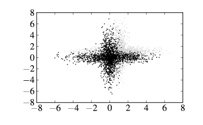
We start by considering the basic two-sample homogeneity test first introduced in Section 2.1. For this, we generate baseline observations distributed as a mixture of two two-dimensional Gaussian densities with common mean (0,0)00(0,0) and diagonal covariance matrices with diagonal terms equal to (4,0.2)40.2(4,0.2) and (0.2,4)0.24(0.2,4), respectively. For the alternative distribution, we generate observations having the same characteristics except that the mean is now equal to 𝒔=(0.5,0.5)𝒔0.50.5\boldsymbol{s}=(0.5,0.5). In this case, n=100𝑛100n=100 and the two groups (baseline and alternative data) are of length n/2=50𝑛250n/2=50. Figure 2 (a) shows a typical example of the data, represented as a two-dimensional scatter plot.

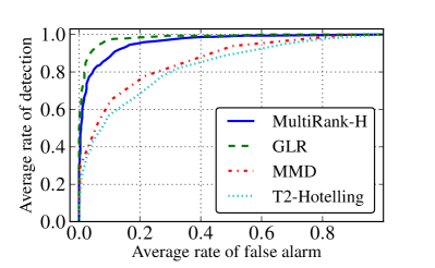
MultiRank-H is compared with three other approaches. The first is the the Maximum Mean Discrepancy (MMD) statistics proposed by Gretton et al. (2006), which is a kernel-based test here used with a Gaussian kernel having a bandwidth given by the median distance between the samples as suggested by Gretton et al. (2006), Désobry et al. (2005) and Harchaoui et al. (2008). The second approach is the classical Hotelling’s T2superscript𝑇2T^{2}-test (Chen and Gupta, 2000, p. 67) which is optimal in the multivariate Gaussian case. The third method is to use the likelihood ratio (LR) test assuming a known structure for the model whose parameters (mean vectors and diagonal terms of the covariance matrices) are estimated using the Expectation-Maximisation algorithm. This latter approach is optimal in this context but is the only one that uses some knowledge about the distribution of the data. These methods are compared through their ROC (Receiver Operating Characteristic) curves, averaged over 100010001000 Monte Carlo replications of the data.

From the results of Section 2.3, we know that, as the covariance matrix of the data is proportional to the identity matrix, the asymptotic performance of Hotelling’s T2superscript𝑇2T^{2}-test does not depend on the particular choice of the shift 𝒔𝒔\boldsymbol{s}, but only on its L2superscript𝐿2L^{2} norm. For the Multirank-H approach the answer is less straightforward as the coordinates of the data are not independent in this example. However, Monte Carlo estimation of the asymptotic performance index ds(𝜹)subscript𝑑𝑠𝜹d_{s}(\boldsymbol{\delta}) in (13) shows that it does not varies by more than 1% with the direction of 𝜹𝜹\boldsymbol{\delta}. We indeed verified that in the setting of Figure 2 the variation in performance with the direction of the shift 𝒔𝒔\boldsymbol{s} is negligible.

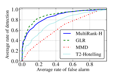
The results displayed in Figure 2(b) show that MultiRank-H is on a par with the LR and outperforms the other two approaches. MMD performs somewhat better than Hotelling’s T2superscript𝑇2T^{2} in this context due to the non-Gaussian nature of the data. Figure 2(c) corresponds to the more difficult setup in which eight-dimensional i.i.d. Gaussian random vectors of variance 2.52superscript2.522.5^{2} are appended to the data described previously. In this case, the data are thus ten-dimensional but the change only affects two coordinates. MultiRank-H is again comparable to the LR, which is still optimal in this case. Note the lack of robustness of MMD which is distinctly dominated by Hotelling’s T2superscript𝑇2T^{2} in this second scenario.

Refer to caption
(a)
Refer to caption Refer to caption
(b) (c)
Figure 2: (a) Example of observations under baseline and alternative distributions, (b) ROC curves for MultiRank-H, MMD, Hotelling’s T2superscript𝑇2T^{2} and LR, (c) Same as (b) with eight-dimensional Gaussian noise padding (that is, with K=10𝐾10K=10).

4.2 Properties of the change-point detection test

In this section, we investigate the properties of the change-point detection test based on the statistic T(n^1)𝑇subscript^𝑛1T(\hat{n}_{1}) resulting from the optimisation of (18). The simulations reported in this section are based on the following common benchmark scenario: under (H0subscript𝐻0H_{0}), that is, in the absence of change, we generate 100 samples from a five-dimensional standard Gaussian distribution. Under (H1subscript𝐻1H_{1}), the observations are similar, except that the common mean of the Gaussian vector changes to 0.3 at a location which is either equal to 1/4 or 1/2 of the observation window, that is, at indices 25 or 50. This scenario corresponds to a simple situation where all coordinates of the data possibly undergo similar upward shifts. The ROC curves that are plotted in the following are based on 2000 replications of the simulated data.

4.2.1 Comparison with marginal decisions

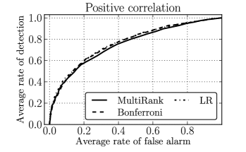
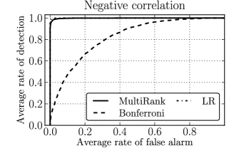
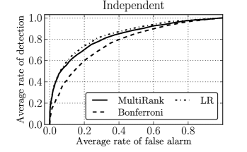
The MultiRank test statistic is obviously based on a combination of marginal rank statistics. Nevertheless, it incorporates two important aspects of the multivariate change-point detection problem: first, detection of simultaneous changes in multiple coordinates should make the presence of an actual change-point more likely, and, second, the existence of dependence between the coordinates should influence the decision. To illustrate these observations, we compare MultiRank with a simpler heuristic approach that combines marginal decisions based on Bonferroni bound, using as test statistic max1kKmax1n1n1Vn,k(n1)subscript1𝑘𝐾subscript1subscript𝑛1𝑛1subscript𝑉𝑛𝑘subscript𝑛1\max_{1\leq k\leq K}\max_{1\leq n_{1}\leq n-1}V_{n,k}(n_{1}). The results obtained with the data-generating mechanism described at the beginning of Section 4.2 are displayed in the leftmost plot of Figure 3. We also compare both approaches in a setting where the covariance matrix of the Gaussian vector is not the identity matrix anymore but a tridiagonal matrix with a common value of 0.450.450.45 (positive correlation) or 0.450.45-0.45 (negative correlation) on the sub- and super-diagonal. The resulting ROC curves are displayed in the middle and right plots of Figure 3, respectively.

The leftmost plot of Figure 3 shows that the approach that combines the marginal statistics by taking into account their correlation, that is MultiRank, outperforms the Bonferroni-type approach. Furthermore, when the coordinates are positively correlated, the rate of detection of the MultiRank method decreases for a given false alarm rate and when negatively correlated, the rate of detection increases. The performance of the Bonferroni-type approach on the other hand does not improve for the negatively correlated data. The MultiRank method captures an important feature of the problem that fails to be exploited by the mere marginal decisions: negative correlations in the data make the detection of simultaneous upward jumps easier while positive correlations render this task more difficult.

Although Figure 3 deals with change-point estimation (which includes the maximisation with respect to the change point position), we note that Corollary 2 of Section 2.3 implies that the performance of the Multirank-H homogeneity test is here comparable to that of the Hotelling’s T2superscript𝑇2T^{2} test as the condition number of the covariance matrices considered in Figures 3 is relatively small (less than 8.1). The Multirank change detection test obviously inherits this property as its performance is nearly indiscernible from that of the LR test for all three choices of the covariance matrix in Figure 3.
Refer to caption Refer to caption Refer to caption
Figure 3: ROC curves for the MultiRank and the Bonferroni-type approaches when the coordinates are independent (left), positively correlated (middle) and negatively correlated (right). The change-point instant is located at 1/4 and 1/2 of the observations window of length 500.
Refer to caption Refer to caption Refer to caption
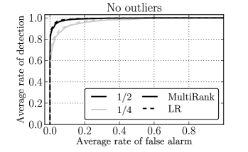
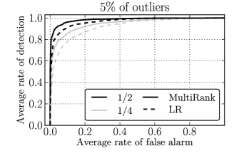
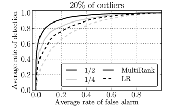
Figure 4: ROC curves for the MultiRank approach and the likelihood-ratio procedure (LR) for three different proportions of outliers (from left to right: 0, 5 and 20%percent\%) when the change-point instant is located at 1/4 and 1/2 of the window of length 500.

4.2.2 Robustness with respect to outliers

Here we illustrate the robustness of the MultiRank approach with respect to outliers in the data by considering the same simulation scenario as in the previous section (with a larger shift of amplitude 0.5) progressively contaminated by large additive outliers. The outliers distribution is the multivariate Gaussian distribution with covariance matrix 10Id510subscriptId510\operatorname{Id}_{5}, instead of Id5subscriptId5\operatorname{Id}_{5} for the baseline distribution (where Id5subscriptId5\operatorname{Id}_{5} refers to the five by five identity matrix). The fraction of outliers is varied between 0, 5 and 20%. The MultiRank approach is compared to the parametric likelihood-ratio based change-point detection test described by Srivastava and Worsley (1986). This latter method, which is itself based on Hotelling’s T2superscript𝑇2T^{2}-test statistic, is optimal in the absence of outliers as the baseline and alternative distributions are both Gaussian. As shown in the leftmost plot of Figure 4, MultiRank has comparable performance with the parametric approach in the case where there are no outliers in the data. However, as shown in the middle and rightmost plots of Figure 4, MultiRank demonstrates its robustness with respect to the presence of outliers as it barely suffers from the presence of additive outliers contrary to the parametric approach.

4.3 Application to genomic hybridisation data

To illustrate the potential of the approach, we consider its application to the segmentation of multiple individual genomic data. We consider the bladder cancer micro-array aCGH dataset studied by Vert and Bleakley (2010) which consists of records of copy-number variations, i.e. abnormal alteration of the quantity of DNA sections.

The objective here is to jointly segment data recorded from different subjects so as to robustly detect regions of frequent deletions or additions of DNA which could be characteristic of cancer. Each of the 57 profiles provides the relative quantity of DNA for 2143 probes measured on 22 chromosomes. We ran the change-point estimation algorithm on each of 22 chromosomes separately, thus processing 22 different 9- to 57-dimensional signals (depending on the selected groups of patients at different stages of cancer) of length 50 to 200 (the number of probes varies for each chromosome).

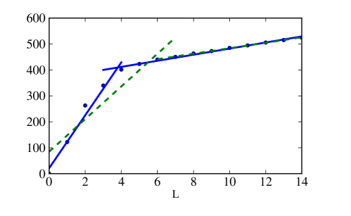
In this paper, we have not considered principled methods for inferring the number of change-points from the data. We describe below an heuristic approach to determine the number of change-points which, despite its simplicity, performs in our experience much better than the use of generic penalties such as AIC or BIC. Values of the statistics IL(n)subscript𝐼𝐿𝑛I_{L}(n), for L=0,,Lmax𝐿0subscript𝐿maxL=0,\dotsc,L_{\text{max}}, are first computed using the procedure described in Section 3.1. The algorithm is based on the principle that in the presence of L1superscript𝐿1L^{\star}\geq 1 change-points, if IL(n)subscript𝐼𝐿𝑛I_{L}(n) is plotted against L𝐿L, the resulting graph can be decomposed into two distinct regions: the first one, for L=0,,L𝐿0superscript𝐿L=0,\dotsc,L^{\star} where the criterion is growing rapidly; and the second one, for L=L,,Lmax𝐿superscript𝐿subscript𝐿maxL=L^{\star},\dotsc,L_{\text{max}}, where the criterion is barely increasing (Lavielle, 2005). Hence, for each possible value of L𝐿L in L=1,,Lmax𝐿1subscript𝐿maxL=1,\dotsc,L_{\text{max}}, we compute least square linear regressions for both parts of the graph (before and after L𝐿L); the estimated number of change-points is the value of L𝐿L that yields the best fit, that is, the value for which the sum of the residual sums of squares computed on both parts of the graph is minimal. For an illustration of this methodology, see Figure 5. The case L=0𝐿0L=0 is treated separately and the procedure described above is used only when the value of the test statistic Wnsubscript𝑊𝑛W_{n} for the presence of a single change-point (see Section 3.2) is significant (p𝑝p-value smaller than 0.1%) based on Theorem 4.
Refer to caption
Figure 5: Determining the optimal number of change-points. Here, the actual number of change-points is L=4superscript𝐿4L^{\star}=4; the optimal regression is displayed in solid lines, while a non-optimal alternative (for L=6𝐿6L=6) is displayed in dashed lines.

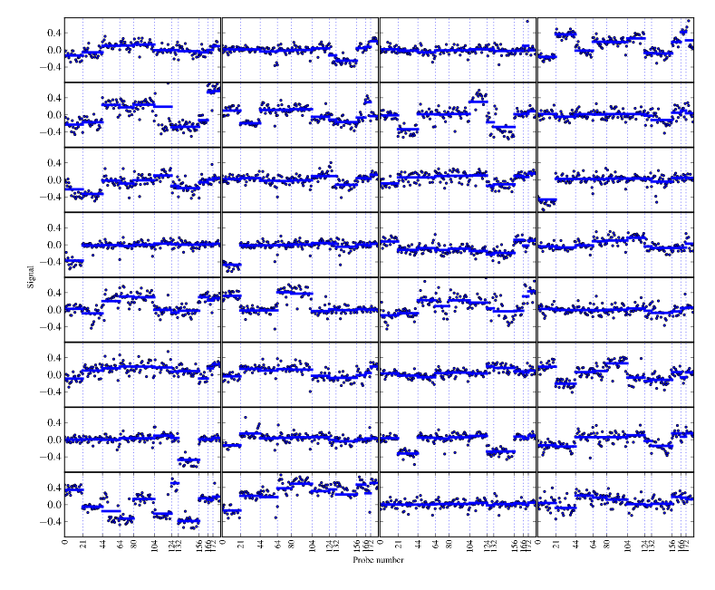
Results are shown for a group of 32 profiles corresponding to Stage T2 of a tumour. In Figure 6 the copy-number data and the segmentation of the whole set of chromosomes is displayed for two particular individuals, together with the corresponding stepwise constant approximations of the data for the 32 individuals (in the bottom of the Figure). Figure 7 details the results pertaining to the 7th chromosome. In both cases, the segmentation result is represented by a signal which is constant (and equal to the mean of the data) within the detected segments. The bottom plot in Figure 6 particularly highlights the fact that several coordinates indeed jump at the same time, suggesting that the joint segmentation model is appropriate. On the other hand, it is also obvious that one cannot assume (see, e.g., the third change-point at index 64 in Figure 7) that all coordinates undergo similar changes. Note also that in this application, the fact that the MultiRank test statistic is properly normalised with respect to the length n𝑛n of the data and their dimension K𝐾K is particularly important: n𝑛n corresponds to the number of probes and varies with each chromosome, K𝐾K represents the number of individuals and varies when considering different groups of subjects.

As a reference, the group fused Lasso algorithm by Bleakley and Vert (2011) outputs similar results. In particular, on the 7th chromosome, change-points are found at positions 21, 44, 65, 102, 107, 112, 124, 132, 156 and 166. On the whole set of chromosomes, 96 change-points are found while the MultiRank estimation procedure outputs 98.

Refer to caption
Refer to caption
Refer to caption
Figure 6: First and second row: copy number data for two different individuals with superimposition of the segmentation. Third row: superimposition of the smoothed bladder tumour aCGH data for 32 individuals in Stage T2 cancer that result from the segmentation. Vertical dashed lines represent the separation between the different chromosomes.
Refer to caption
Figure 7: Data for 32 individuals in Stage T2 bladder cancer with superimposed segmentation for chromosome 7. 10 change-points were estimated and the dashed vertical lines correspond to the estimated segment boundaries.

5 Conclusion

We proposed an approach for retrospective detection of multiple changes in multivariate data. The basic idea, used for homogeneity testing when the data groupings are known, is an extension of well-known marginal rank based tests (Wilcoxon/Mann-Whitney and Kruskal-Wallis) based on the idea originally proposed by Wei and Lachin (1984). The use of this approach for change-point detection (when the segments boundaries are unknown) was shown to be computationally feasible. In addition, it incorporates important aspects of the problem, in particular the fact that simultaneous detections in different coordinates make the presence of an actual change more likely. The method was shown to be robust against various alternatives and on a par with optimal methods in benchmark cases. The approach can also be straightforwardly modified to deal with ordinal data, missing or censored values.

To improve the method, it would be desirable to provide significance levels for the change-point detection test when used to detect more than a single potential change-point. We believe that by considering the normalisation used to define the statistic Wnsubscript𝑊𝑛W_{n} in Section 3.2, it is possible to study the asymptotic behaviour of the change-point detection statistic in the general case. This being said, the difference between the two forms of normalisation could be more significant when applied to more than two segments. On a different level, one should obviously consider more principled approaches for selecting the number of change-points. General-purpose penalisation schemes could be used but we feel that novel ideas need to be developed specifically for the change-point problem given the specific nature of over- and under-estimating the number of change-points. For instance, in many practical applications the significance of over-estimating the number of change-points depends not only on the number of spurious segments but also on their locations. Traditional approaches based on complexity penalties (Bai and Perron, 2003), Bayesian methods (Fearnhead, 2006) and sparsity-based criterions (Harchaoui and Lévy-Leduc, 2010; Vert and Bleakley, 2010) are already available but there is certainly room for new developments in these fields.

Appendix A Appendix: Proof of Theorem 1

The proof is based on the Hoeffding decomposition of Un,k(n1)subscript𝑈𝑛𝑘subscript𝑛1U_{n,k}(n_{1}) for each k𝑘k in {1,,K}1𝐾\{1,\dotsc,K\}. For further details on the Hoeffding decomposition, we refer the reader to Chapters 11 and 12 of van der Vaart (1998). For each k𝑘k in {1,,K}1𝐾\{1,\dotsc,K\}, let h1,k(y)=h(x,y)𝑑Fk(x)subscript1𝑘𝑦𝑥𝑦differential-dsubscript𝐹𝑘𝑥h_{1,k}(y)=\int\!h(x,y)dF_{k}(x) and h~1,k(x)=h(x,y)𝑑Fk(y)subscript~1𝑘𝑥𝑥𝑦differential-dsubscript𝐹𝑘𝑦\tilde{h}_{1,k}(x)=\int\!h(x,y)dF_{k}(y), where hh is defined by h(x,y)=𝟏(xy)𝟏(yx)𝑥𝑦1𝑥𝑦1𝑦𝑥h(x,y)=\mathbf{1}(x\leq y)-\mathbf{1}(y\leq x). By the continuity of Fksubscript𝐹𝑘F_{k}, h1,k(y)=2Fk(y)1subscript1𝑘𝑦2subscript𝐹𝑘𝑦1h_{1,k}(y)=2F_{k}(y)-1 and h~1,k(x)=12Fk(x)subscript~1𝑘𝑥12subscript𝐹𝑘𝑥\tilde{h}_{1,k}(x)=1-2F_{k}(x). The Hoeffding decomposition of Un,k(n1)subscript𝑈𝑛𝑘subscript𝑛1U_{n,k}(n_{1}) can thus be written as Un,k(n1)=U^n,k(n1)+Rn,k(n1)subscript𝑈𝑛𝑘subscript𝑛1subscript^𝑈𝑛𝑘subscript𝑛1subscript𝑅𝑛𝑘subscript𝑛1U_{n,k}(n_{1})=\hat{U}_{n,k}(n_{1})+R_{n,k}(n_{1}), where

U^n,k(n1)=n1nn1(nn1)j=n1+1nh1,k(Xj,k)+nn1nn1(nn1)i=1n1h~1,k(Xi,k),subscript^𝑈𝑛𝑘subscript𝑛1subscript𝑛1𝑛subscript𝑛1𝑛subscript𝑛1superscriptsubscript𝑗subscript𝑛11𝑛subscript1𝑘subscript𝑋𝑗𝑘𝑛subscript𝑛1𝑛subscript𝑛1𝑛subscript𝑛1superscriptsubscript𝑖1subscript𝑛1subscript~1𝑘subscript𝑋𝑖𝑘\displaystyle\hat{U}_{n,k}(n_{1})=\frac{n_{1}}{\sqrt{nn_{1}(n-n_{1})}}\sum_{j=n_{1}+1}^{n}h_{1,k}(X_{j,k})+\frac{n-n_{1}}{\sqrt{nn_{1}(n-n_{1})}}\sum_{i=1}^{n_{1}}\tilde{h}_{1,k}(X_{i,k})\;, (21)
Rn,k(n1)=1nn1(nn1)i=1n1j=n1+1n[h(Xi,k,Xj,k)h~1,k(Xi,k)h1,k(Xj,k)].subscript𝑅𝑛𝑘subscript𝑛11𝑛subscript𝑛1𝑛subscript𝑛1superscriptsubscript𝑖1subscript𝑛1superscriptsubscript𝑗subscript𝑛11𝑛delimited-[]subscript𝑋𝑖𝑘subscript𝑋𝑗𝑘subscript~1𝑘subscript𝑋𝑖𝑘subscript1𝑘subscript𝑋𝑗𝑘\displaystyle R_{n,k}(n_{1})=\frac{1}{\sqrt{nn_{1}(n-n_{1})}}\sum_{i=1}^{n_{1}}\sum_{j=n_{1}+1}^{n}\![h(X_{i,k},X_{j,k})-\tilde{h}_{1,k}(X_{i,k})-h_{1,k}(X_{j,k})]\;. (22)

We first prove that Un,k(n1)=U^n,k(n1)+op(1)subscript𝑈𝑛𝑘subscript𝑛1subscript^𝑈𝑛𝑘subscript𝑛1subscript𝑜𝑝1U_{n,k}(n_{1})=\hat{U}_{n,k}(n_{1})+o_{p}(1) by showing that Var[Rn,k(n1)]0Varsubscript𝑅𝑛𝑘subscript𝑛10\operatorname*{Var}[R_{n,k}(n_{1})]\to 0, as n𝑛n tends to infinity. Using that 𝔼[Un,k(n1)]=𝔼[U^n,k(n1)]=0𝔼delimited-[]subscript𝑈𝑛𝑘subscript𝑛1𝔼delimited-[]subscript^𝑈𝑛𝑘subscript𝑛10\mathbb{E}[U_{n,k}(n_{1})]=\mathbb{E}[\hat{U}_{n,k}(n_{1})]=0, we obtain that Var[Rn,k(n1)]=Var[Un,k(n1)U^n,k(n1)]=𝔼[Un,k2(n1)]+𝔼[U^n,k2(n1)]2𝔼[Un,k(n1)U^n,k(n1)].Varsubscript𝑅𝑛𝑘subscript𝑛1Varsubscript𝑈𝑛𝑘subscript𝑛1subscript^𝑈𝑛𝑘subscript𝑛1𝔼delimited-[]superscriptsubscript𝑈𝑛𝑘2subscript𝑛1𝔼delimited-[]superscriptsubscript^𝑈𝑛𝑘2subscript𝑛12𝔼delimited-[]subscript𝑈𝑛𝑘subscript𝑛1subscript^𝑈𝑛𝑘subscript𝑛1\operatorname*{Var}[R_{n,k}(n_{1})]=\operatorname*{Var}[U_{n,k}(n_{1})-\hat{U}_{n,k}(n_{1})]=\mathbb{E}[U_{n,k}^{2}(n_{1})]+\mathbb{E}[\hat{U}_{n,k}^{2}(n_{1})]-2\mathbb{E}[U_{n,k}(n_{1})\hat{U}_{n,k}(n_{1})]. By independence of the (Xi,k)1insubscriptsubscript𝑋𝑖𝑘1𝑖𝑛(X_{i,k})_{1\leq i\leq n}, we obtain that

𝔼[U^n,k2(n1)]=n12nn1(nn1)j=n1+1n𝔼[h1,k(Xj,k)2]+(nn1)2nn1(nn1)i=1n1𝔼[h~1,k(Xi,k)2].𝔼delimited-[]superscriptsubscript^𝑈𝑛𝑘2subscript𝑛1superscriptsubscript𝑛12𝑛subscript𝑛1𝑛subscript𝑛1superscriptsubscript𝑗subscript𝑛11𝑛𝔼delimited-[]subscript1𝑘superscriptsubscript𝑋𝑗𝑘2superscript𝑛subscript𝑛12𝑛subscript𝑛1𝑛subscript𝑛1superscriptsubscript𝑖1subscript𝑛1𝔼delimited-[]subscript~1𝑘superscriptsubscript𝑋𝑖𝑘2\mathbb{E}[\hat{U}_{n,k}^{2}(n_{1})]=\frac{n_{1}^{2}}{nn_{1}(n-n_{1})}\sum_{j=n_{1}+1}^{n}\mathbb{E}[h_{1,k}(X_{j,k})^{2}]+\frac{(n-n_{1})^{2}}{nn_{1}(n-n_{1})}\sum_{i=1}^{n_{1}}\mathbb{E}[\tilde{h}_{1,k}(X_{i,k})^{2}]. (23)

Using that

𝔼[h1,k(Xi,k)2]=4𝔼[(Fk(X1,k)1/2)2]=4Var(𝒰)=1/3,𝔼delimited-[]subscript1𝑘superscriptsubscript𝑋𝑖𝑘24𝔼delimited-[]superscriptsubscript𝐹𝑘subscript𝑋1𝑘1224Var𝒰13\mathbb{E}[h_{1,k}(X_{i,k})^{2}]=4\mathbb{E}[(F_{k}(X_{1,k})-1/2)^{2}]=4\operatorname*{Var}(\mathcal{U})=1/3\;, (24)

where 𝒰𝒰\mathcal{U} has a uniform distribution on [0,1]01[0,1], we get, on the one hand, that

𝔼[U^n,k2(n1)]=n12(nn1)3nn1(nn1)+(nn1)2n13nn1(nn1)=1/3.𝔼delimited-[]superscriptsubscript^𝑈𝑛𝑘2subscript𝑛1superscriptsubscript𝑛12𝑛subscript𝑛13𝑛subscript𝑛1𝑛subscript𝑛1superscript𝑛subscript𝑛12subscript𝑛13𝑛subscript𝑛1𝑛subscript𝑛113\mathbb{E}[\hat{U}_{n,k}^{2}(n_{1})]=\frac{n_{1}^{2}(n-n_{1})}{3nn_{1}(n-n_{1})}+\frac{(n-n_{1})^{2}n_{1}}{3nn_{1}(n-n_{1})}=1/3\;. (25)

On the other hand

𝔼[Un,k2(n1)]=1nn1(nn1)i=1n1j=n1+1n𝔼[h(Xi,k,Xj,k)2]+1nn1(nn1)1iin1j=n1+1n𝔼[h(Xi,k,Xj,k)h(Xi,k,Xj,k)]+1nn1(nn1)i=1n1n1+1jjn𝔼[h(Xi,k,Xj,k)h(Xi,k,Xj,k)].𝔼delimited-[]superscriptsubscript𝑈𝑛𝑘2subscript𝑛11𝑛subscript𝑛1𝑛subscript𝑛1superscriptsubscript𝑖1subscript𝑛1superscriptsubscript𝑗subscript𝑛11𝑛𝔼delimited-[]superscriptsubscript𝑋𝑖𝑘subscript𝑋𝑗𝑘21𝑛subscript𝑛1𝑛subscript𝑛1subscript1𝑖superscript𝑖subscript𝑛1superscriptsubscript𝑗subscript𝑛11𝑛𝔼delimited-[]subscript𝑋𝑖𝑘subscript𝑋𝑗𝑘subscript𝑋superscript𝑖𝑘subscript𝑋𝑗𝑘1𝑛subscript𝑛1𝑛subscript𝑛1superscriptsubscript𝑖1subscript𝑛1subscriptsubscript𝑛11𝑗superscript𝑗𝑛𝔼delimited-[]subscript𝑋𝑖𝑘subscript𝑋𝑗𝑘subscript𝑋𝑖𝑘subscript𝑋superscript𝑗𝑘\mathbb{E}[U_{n,k}^{2}(n_{1})]=\frac{1}{nn_{1}(n-n_{1})}\sum_{i=1}^{n_{1}}\sum_{j=n_{1}+1}^{n}\mathbb{E}[h(X_{i,k},X_{j,k})^{2}]\\ +\frac{1}{nn_{1}(n-n_{1})}\sum_{1\leq i\neq i^{\prime}\leq n_{1}}\sum_{j=n_{1}+1}^{n}\mathbb{E}[h(X_{i,k},X_{j,k})h(X_{i^{\prime},k},X_{j,k})]\\ +\frac{1}{nn_{1}(n-n_{1})}\sum_{i=1}^{n_{1}}\sum_{n_{1}+1\leq j\neq j^{\prime}\leq n}\mathbb{E}[h(X_{i,k},X_{j,k})h(X_{i,k},X_{j^{\prime},k})]\;. (26)

We separately study the three terms of the r.h.s of (26). Using that (Xi,k)1insubscriptsubscript𝑋𝑖𝑘1𝑖𝑛(X_{i,k})_{1\leq i\leq n} are i.i.d. , we get

1nn1(nn1)i=1n1j=n1+1n𝔼[h(Xi,k,Xj,k)2]=n1(nn1)nn1(nn1)𝔼[h(X1,k,Xn1+1,k)2]0,as n.formulae-sequence1𝑛subscript𝑛1𝑛subscript𝑛1superscriptsubscript𝑖1subscript𝑛1superscriptsubscript𝑗subscript𝑛11𝑛𝔼delimited-[]superscriptsubscript𝑋𝑖𝑘subscript𝑋𝑗𝑘2subscript𝑛1𝑛subscript𝑛1𝑛subscript𝑛1𝑛subscript𝑛1𝔼delimited-[]superscriptsubscript𝑋1𝑘subscript𝑋subscript𝑛11𝑘20as n\frac{1}{nn_{1}(n-n_{1})}\sum_{i=1}^{n_{1}}\sum_{j=n_{1}+1}^{n}\mathbb{E}[h(X_{i,k},X_{j,k})^{2}]=\frac{n_{1}(n-n_{1})}{nn_{1}(n-n_{1})}\mathbb{E}[h(X_{1,k},X_{n_{1}+1,k})^{2}]\to 0,\;\text{as $n\to\infty$}\;. (27)

Then, by continuity of Fksubscript𝐹𝑘F_{k}, we have

1nn1(nn1)1iin1j=n1+1n𝔼[h(Xi,k,Xj,k)h(Xi,k,Xj,k)]=(n12n1)(nn1)nn1(nn1)(2Fk(y)1)(2Fk(y)1)𝑑Fk(y)=n1(n11)(nn1)3nn1(nn1).1𝑛subscript𝑛1𝑛subscript𝑛1subscript1𝑖superscript𝑖subscript𝑛1superscriptsubscript𝑗subscript𝑛11𝑛𝔼delimited-[]subscript𝑋𝑖𝑘subscript𝑋𝑗𝑘subscript𝑋superscript𝑖𝑘subscript𝑋𝑗𝑘superscriptsubscript𝑛12subscript𝑛1𝑛subscript𝑛1𝑛subscript𝑛1𝑛subscript𝑛12subscript𝐹𝑘𝑦12subscript𝐹𝑘𝑦1differential-dsubscript𝐹𝑘𝑦subscript𝑛1subscript𝑛11𝑛subscript𝑛13𝑛subscript𝑛1𝑛subscript𝑛1\frac{1}{nn_{1}(n-n_{1})}\sum_{1\leq i\neq i^{\prime}\leq n_{1}}\sum_{j=n_{1}+1}^{n}\mathbb{E}[h(X_{i,k},X_{j,k})h(X_{i^{\prime},k},X_{j,k})]\\ =\frac{(n_{1}^{2}-n_{1})(n-n_{1})}{nn_{1}(n-n_{1})}\int(2F_{k}(y)-1)(2F_{k}(y)-1)dF_{k}(y)=\frac{n_{1}(n_{1}-1)(n-n_{1})}{3nn_{1}(n-n_{1})}\;. (28)

Using similar arguments, the last term of the r.h.s of (26) is equal to n1(nn1)(nn11)/(3nn1(nn1))subscript𝑛1𝑛subscript𝑛1𝑛subscript𝑛113𝑛subscript𝑛1𝑛subscript𝑛1n_{1}(n-n_{1})(n-n_{1}-1)/(3nn_{1}(n-n_{1})). With (27) and (28), we obtain

𝔼[Un,k2(n1)]1/3,as n.𝔼delimited-[]superscriptsubscript𝑈𝑛𝑘2subscript𝑛113as n\mathbb{E}[U_{n,k}^{2}(n_{1})]\to 1/3,\;\text{as $n\to\infty$}. (29)

Since 𝔼[Un,k(n1)U^n,k(n1)]1/3𝔼delimited-[]subscript𝑈𝑛𝑘subscript𝑛1subscript^𝑈𝑛𝑘subscript𝑛113\mathbb{E}[U_{n,k}(n_{1})\hat{U}_{n,k}(n_{1})]\to 1/3, as n𝑛n\to\infty, (25) and (29) lead to Var[Rn,k(n1)]0Varsubscript𝑅𝑛𝑘subscript𝑛10\operatorname*{Var}[R_{n,k}(n_{1})]\to 0 and thus Un,k(n1)=U^n,k(n1)+op(1)subscript𝑈𝑛𝑘subscript𝑛1subscript^𝑈𝑛𝑘subscript𝑛1subscript𝑜𝑝1U_{n,k}(n_{1})=\hat{U}_{n,k}(n_{1})+o_{p}(1), as n𝑛n tends to infinity. The multivariate central limit theorem then yields (Un,1(n1),,Un,K(n1))𝒩(0,Σ),superscriptsubscript𝑈𝑛1subscript𝑛1subscript𝑈𝑛𝐾subscript𝑛1𝒩0Σ(U_{n,1}(n_{1}),\dotsc,U_{n,K}(n_{1}))^{\prime}\to\mathcal{N}(0,\Sigma)\;, where the (k,k)𝑘superscript𝑘(k,k^{\prime})th entry of ΣΣ\Sigma is given by Σkk=limn𝔼[U^n,k(n1)U^n,k(n1)]subscriptΣ𝑘superscript𝑘subscript𝑛𝔼delimited-[]subscript^𝑈𝑛𝑘subscript𝑛1subscript^𝑈𝑛superscript𝑘subscript𝑛1\Sigma_{kk^{\prime}}=\lim_{n\to\infty}\mathbb{E}[\hat{U}_{n,k}(n_{1})\hat{U}_{n,k^{\prime}}(n_{1})]. Using that the (Xi,k)1insubscriptsubscript𝑋𝑖𝑘1𝑖𝑛(X_{i,k})_{1\leq i\leq n} are i.i.d., we obtain that

𝔼[U^n,k(n1)U^n,k(n1)]=4n12nn1(nn1)j=n1+1n𝔼[{Fk(Xj,k)1/2}{Fk(Xj,k)1/2}]+4(nn1)2nn1(nn1)i=1n1𝔼[{Fk(Xi,k)1/2}{Fk(Xi,k)1/2}]=4Cov(Fk(X1,k),Fk(X1,k)).𝔼delimited-[]subscript^𝑈𝑛𝑘subscript𝑛1subscript^𝑈𝑛superscript𝑘subscript𝑛14superscriptsubscript𝑛12𝑛subscript𝑛1𝑛subscript𝑛1superscriptsubscript𝑗subscript𝑛11𝑛𝔼delimited-[]subscript𝐹𝑘subscript𝑋𝑗𝑘12subscript𝐹superscript𝑘subscript𝑋𝑗superscript𝑘124superscript𝑛subscript𝑛12𝑛subscript𝑛1𝑛subscript𝑛1superscriptsubscript𝑖1subscript𝑛1𝔼delimited-[]subscript𝐹𝑘subscript𝑋𝑖𝑘12subscript𝐹superscript𝑘subscript𝑋𝑖superscript𝑘124Covsubscript𝐹𝑘subscript𝑋1𝑘subscript𝐹superscript𝑘subscript𝑋1superscript𝑘\mathbb{E}[\hat{U}_{n,k}(n_{1})\hat{U}_{n,k^{\prime}}(n_{1})]=\frac{4n_{1}^{2}}{nn_{1}(n-n_{1})}\sum_{j=n_{1}+1}^{n}\mathbb{E}[\{F_{k}(X_{j,k})-1/2\}\{F_{k^{\prime}}(X_{j,k^{\prime}})-1/2\}]\\ +\frac{4(n-n_{1})^{2}}{nn_{1}(n-n_{1})}\sum_{i=1}^{n_{1}}\mathbb{E}[\{F_{k}(X_{i,k})-1/2\}\{F_{k^{\prime}}(X_{i,k^{\prime}})-1/2\}]\\ =4\operatorname*{Cov}\left(F_{k}(X_{1,k}),F_{k^{\prime}}(X_{1,k^{\prime}})\right)\;.

Thus, Σ1/2(Un,1(n1),,Un,K(n1))d𝒩(0,IdK)superscript𝑑superscriptΣ12superscriptsubscript𝑈𝑛1subscript𝑛1subscript𝑈𝑛𝐾subscript𝑛1𝒩0subscriptId𝐾\Sigma^{-1/2}(U_{n,1}(n_{1}),\dotsc,U_{n,K}(n_{1}))^{\prime}\stackrel{{\scriptstyle{d}}}{{\longrightarrow}}\mathcal{N}(0,\operatorname{Id}_{K}). Since Σ^npΣsuperscript𝑝subscript^Σ𝑛Σ\hat{\Sigma}_{n}\stackrel{{\scriptstyle p}}{{\longrightarrow}}\Sigma, we deduce from Slutsky’s Theorem that Σ^n1/2(Un,1(n1),,Un,K(n1))d𝒩(0,IdK)superscript𝑑superscriptsubscript^Σ𝑛12superscriptsubscript𝑈𝑛1subscript𝑛1subscript𝑈𝑛𝐾subscript𝑛1𝒩0subscriptId𝐾\hat{\Sigma}_{n}^{-1/2}(U_{n,1}(n_{1}),\dotsc,U_{n,K}(n_{1}))^{\prime}\stackrel{{\scriptstyle{d}}}{{\longrightarrow}}\mathcal{N}(0,\operatorname{Id}_{K}), which concludes the proof.

Appendix B Appendix: Proof of Theorem 2

Using that Rj(k)=i=1n𝟏(Xi,kXj,k)superscriptsubscript𝑅𝑗𝑘superscriptsubscript𝑖1𝑛1subscript𝑋𝑖𝑘subscript𝑋𝑗𝑘R_{j}^{(k)}=\sum_{i=1}^{n}\mathbf{1}(X_{i,k}\leq X_{j,k}), we obtain that

R¯(k)n+12=1n+1n(j=n+1n+1i=1n𝟏(Xi,kXj,k))n+12=1n+1nj=n+1n+1iji=1n[𝟏(Xi,kXj,k)1/2].superscriptsubscript¯𝑅𝑘𝑛121subscript𝑛1subscript𝑛superscriptsubscript𝑗subscript𝑛1subscript𝑛1superscriptsubscript𝑖1𝑛1subscript𝑋𝑖𝑘subscript𝑋𝑗𝑘𝑛121subscript𝑛1subscript𝑛superscriptsubscript𝑗subscript𝑛1subscript𝑛1superscriptsubscriptsuperscript𝑖𝑗𝑖1𝑛delimited-[]1subscript𝑋𝑖𝑘subscript𝑋𝑗𝑘12\bar{R}_{\ell}^{(k)}-\frac{n+1}{2}=\frac{1}{n_{\ell+1}-n_{\ell}}\left(\sum_{j=n_{\ell}+1}^{n_{\ell+1}}\sum_{i=1}^{n}\mathbf{1}(X_{i,k}\leq X_{j,k})\right)-\frac{n+1}{2}\\ =\frac{1}{n_{\ell+1}-n_{\ell}}\sum_{j=n_{\ell}+1}^{n_{\ell+1}}\sum_{\stackrel{{\scriptstyle i=1}}{{i\neq j}}}^{n}\left[\mathbf{1}(X_{i,k}\leq X_{j,k})-1/2\right]\;. (30)

Let h(x,y)=𝟏(xy)𝑥𝑦1𝑥𝑦h(x,y)=\mathbf{1}(x\leq y), h1,k(y)=𝟏(xy)dFk(x)subscript1𝑘𝑦1𝑥𝑦dsubscript𝐹𝑘𝑥h_{1,k}(y)=\int\mathbf{1}(x\leq y)\textrm{d}F_{k}(x) and h2,k(x)=𝟏(xy)dFk(y).subscript2𝑘𝑥1𝑥𝑦dsubscript𝐹𝑘𝑦h_{2,k}(x)=\int\mathbf{1}(x\leq y)\textrm{d}F_{k}(y). By continuity of Fksubscript𝐹𝑘F_{k}: h1,k(y)=Fk(y)subscript1𝑘𝑦subscript𝐹𝑘𝑦h_{1,k}(y)=F_{k}(y) and h2,k(x)=1Fk(x).subscript2𝑘𝑥1subscript𝐹𝑘𝑥h_{2,k}(x)=1-F_{k}(x). Using the notation:

(k)=(n+1n)1/2/n(R¯(k)(n+1)/2),superscriptsubscript𝑘superscriptsubscript𝑛1subscript𝑛12𝑛superscriptsubscript¯𝑅𝑘𝑛12\mathcal{R}_{\ell}^{(k)}=(n_{\ell+1}-n_{\ell})^{1/2}/n(\bar{R}_{\ell}^{(k)}-(n+1)/2)\;,

the Hoeffding decomposition yields

(k)=(n+1n)1/2n[n1n+1nj=n+1n+1(h1,k(Xj,k)1/2)+n+1n1n+1ni=1n(h2,k(Xi,k)1/2)]+(n+1n)1/2n[1n+1nj=n+1n+1iji=1n{h(Xi,k,Xj,k)h1,k(Xj,k)h2,k(Xi,k)+1/2}]=def,1(k)+,2(k)+,3(k).superscriptsubscript𝑘superscriptsubscript𝑛1subscript𝑛12𝑛delimited-[]𝑛1subscript𝑛1subscript𝑛superscriptsubscript𝑗subscript𝑛1subscript𝑛1subscript1𝑘subscript𝑋𝑗𝑘12subscript𝑛1subscript𝑛1subscript𝑛1subscript𝑛superscriptsubscript𝑖1𝑛subscript2𝑘subscript𝑋𝑖𝑘12superscriptsubscript𝑛1subscript𝑛12𝑛delimited-[]1subscript𝑛1subscript𝑛superscriptsubscript𝑗subscript𝑛1subscript𝑛1superscriptsubscriptsuperscript𝑖𝑗𝑖1𝑛subscript𝑋𝑖𝑘subscript𝑋𝑗𝑘subscript1𝑘subscript𝑋𝑗𝑘subscript2𝑘subscript𝑋𝑖𝑘12superscriptdefsuperscriptsubscript1𝑘superscriptsubscript2𝑘superscriptsubscript3𝑘\mathcal{R}_{\ell}^{(k)}=\frac{(n_{\ell+1}-n_{\ell})^{1/2}}{n}\left[\frac{n-1}{n_{\ell+1}-n_{\ell}}\sum_{j=n_{\ell}+1}^{n_{\ell+1}}(h_{1,k}(X_{j,k})-1/2)+\frac{n_{\ell+1}-n_{\ell}-1}{n_{\ell+1}-n_{\ell}}\sum_{i=1}^{n}(h_{2,k}(X_{i,k})-1/2)\right]\\ +\frac{(n_{\ell+1}-n_{\ell})^{1/2}}{n}\left[\frac{1}{n_{\ell+1}-n_{\ell}}\sum_{j=n_{\ell}+1}^{n_{\ell+1}}\sum_{\stackrel{{\scriptstyle i=1}}{{i\neq j}}}^{n}\left\{h(X_{i,k},X_{j,k})-h_{1,k}(X_{j,k})-h_{2,k}(X_{i,k})+1/2\right\}\right]\\ \stackrel{{\scriptstyle\textrm{def}}}{{=}}\mathcal{R}_{\ell,1}^{(k)}+\mathcal{R}_{\ell,2}^{(k)}+\mathcal{R}_{\ell,3}^{(k)}\;. (31)

Note that ,3(k)=op(1)superscriptsubscript3𝑘subscript𝑜𝑝1\mathcal{R}_{\ell,3}^{(k)}=o_{p}(1), as n𝑛n tends to infinity, since it can be proved that Var(,3(k))=Var[(k)(,1(k)+,2(k))]0Varsuperscriptsubscript3𝑘Varsuperscriptsubscript𝑘superscriptsubscript1𝑘superscriptsubscript2𝑘0\operatorname*{Var}(\mathcal{R}_{\ell,3}^{(k)})=\operatorname*{Var}[\mathcal{R}_{\ell}^{(k)}-(\mathcal{R}_{\ell,1}^{(k)}+\mathcal{R}_{\ell,2}^{(k)})]\to 0, as n𝑛n tends to infinity. Thus, (31) can be rewritten as

(k)=n1n(n+1n)1/2j=n+1n+1(Fk(Xj,k)1/2)+n+1n1n(n+1n)1/2i=1n(1/2Fk(Xi,k))+op(1).superscriptsubscript𝑘𝑛1𝑛superscriptsubscript𝑛1subscript𝑛12superscriptsubscript𝑗subscript𝑛1subscript𝑛1subscript𝐹𝑘subscript𝑋𝑗𝑘12subscript𝑛1subscript𝑛1𝑛superscriptsubscript𝑛1subscript𝑛12superscriptsubscript𝑖1𝑛12subscript𝐹𝑘subscript𝑋𝑖𝑘subscript𝑜𝑝1\mathcal{R}_{\ell}^{(k)}=\frac{n-1}{n(n_{\ell+1}-n_{\ell})^{1/2}}\sum_{j=n_{\ell}+1}^{n_{\ell+1}}(F_{k}(X_{j,k})-1/2)+\frac{n_{\ell+1}-n_{\ell}-1}{n(n_{\ell+1}-n_{\ell})^{1/2}}\sum_{i=1}^{n}(1/2-F_{k}(X_{i,k}))+o_{p}(1)\;.

Since i=1n(1/2Fk(Xi,k))=p=0L1j=np+1np+1(1/2Fk(Xj,k))superscriptsubscript𝑖1𝑛12subscript𝐹𝑘subscript𝑋𝑖𝑘superscriptsubscript𝑝0𝐿1superscriptsubscript𝑗subscript𝑛𝑝1subscript𝑛𝑝112subscript𝐹𝑘subscript𝑋𝑗𝑘\sum_{i=1}^{n}(1/2-F_{k}(X_{i,k}))=\sum_{p=0}^{L-1}\sum_{j=n_{p}+1}^{n_{p+1}}(1/2-F_{k}(X_{j,k})),

(k)=n(n+1n)n(n+1n)1/2j=n+1n+1(Fk(Xj,k)1/2)n+1n1n(n+1n)1/2pp=0L1j=np+1np+1(Fk(Xj,k1/2))+op(1)=defUk(n,n+1)+op(1).superscriptsubscript𝑘𝑛subscript𝑛1subscript𝑛𝑛superscriptsubscript𝑛1subscript𝑛12superscriptsubscript𝑗subscript𝑛1subscript𝑛1subscript𝐹𝑘subscript𝑋𝑗𝑘12subscript𝑛1subscript𝑛1𝑛superscriptsubscript𝑛1subscript𝑛12superscriptsubscriptsuperscript𝑝𝑝0𝐿1superscriptsubscript𝑗subscript𝑛𝑝1subscript𝑛𝑝1subscript𝐹𝑘subscript𝑋𝑗𝑘12subscript𝑜𝑝1superscriptdefsubscript𝑈𝑘subscript𝑛subscript𝑛1subscript𝑜𝑝1\mathcal{R}_{\ell}^{(k)}=\frac{n-(n_{\ell+1}-n_{\ell})}{n(n_{\ell+1}-n_{\ell})^{1/2}}\sum_{j=n_{\ell}+1}^{n_{\ell+1}}(F_{k}(X_{j,k})-1/2)-\frac{n_{\ell+1}-n_{\ell}-1}{n(n_{\ell+1}-n_{\ell})^{1/2}}\sum_{\stackrel{{\scriptstyle p=0}}{{p\neq\ell}}}^{L-1}\sum_{j=n_{p}+1}^{n_{p+1}}(F_{k}(X_{j,k}-1/2))+o_{p}(1)\\ \stackrel{{\scriptstyle\textrm{def}}}{{=}}U_{k}(n_{\ell},n_{\ell+1})+o_{p}(1)\;.

Observe that, for a fixed \ell in {0,,L1}0𝐿1\{0,\dots,L-1\} and k,k𝑘superscript𝑘k,k^{\prime} in {1,,K}1𝐾\{1,\dots,K\}, we get, as n𝑛n tends to infinity,

4Cov(Uk(n,n+1),Uk(n,n+1))=Σkk[(1(n+1n)n)2+pp=0L1(n+1n1)2(np+1np)n2(n+1n)](1t+1)Σkk,4Covsubscript𝑈𝑘subscript𝑛subscript𝑛1subscript𝑈superscript𝑘subscript𝑛subscript𝑛1subscriptΣ𝑘superscript𝑘delimited-[]superscript1subscript𝑛1subscript𝑛𝑛2superscriptsubscriptsuperscript𝑝𝑝0𝐿1superscriptsubscript𝑛1subscript𝑛12subscript𝑛𝑝1subscript𝑛𝑝superscript𝑛2subscript𝑛1subscript𝑛1subscript𝑡1subscriptΣ𝑘superscript𝑘4\operatorname*{Cov}(U_{k}(n_{\ell},n_{\ell+1}),U_{k^{\prime}}(n_{\ell},n_{\ell+1}))=\\ \Sigma_{kk^{\prime}}\left[\left(1-\frac{(n_{\ell+1}-n_{\ell})}{n}\right)^{2}+\sum_{\stackrel{{\scriptstyle p=0}}{{p\neq\ell}}}^{L-1}\frac{(n_{\ell+1}-n_{\ell}-1)^{2}(n_{p+1}-n_{p})}{n^{2}(n_{\ell+1}-n_{\ell})}\right]\to(1-t_{\ell+1})\Sigma_{kk^{\prime}}\;, (32)

where we have used that pp=0L1(np+1np)=n(n+1n).superscriptsubscriptsuperscript𝑝𝑝0𝐿1subscript𝑛𝑝1subscript𝑛𝑝𝑛subscript𝑛1subscript𝑛\sum_{\stackrel{{\scriptstyle p=0}}{{p\neq\ell}}}^{L-1}(n_{p+1}-n_{p})=n-(n_{\ell+1}-n_{\ell}). In the same way, for fixed k,k𝑘superscript𝑘k,k^{\prime} in {1,,K}1𝐾\{1,\dots,K\} and superscript\ell\neq\ell^{\prime} in {0,,L1}0𝐿1\{0,\dots,L-1\}, we obtain, as n𝑛n tends to infinity,

4Cov(Uk(n,n+1),Uk(n,n+1))t+1t+1Σkk.4Covsubscript𝑈𝑘subscript𝑛subscript𝑛1subscript𝑈superscript𝑘subscript𝑛superscriptsubscript𝑛superscript1subscript𝑡1subscript𝑡superscript1subscriptΣ𝑘superscript𝑘4\operatorname*{Cov}(U_{k}(n_{\ell},n_{\ell+1}),U_{k^{\prime}}(n_{\ell^{\prime}},n_{\ell^{\prime}+1}))\to-\sqrt{t_{\ell+1}t_{\ell^{\prime}+1}}\Sigma_{kk^{\prime}}\;. (33)

Let

R¯n=2((n1n0)1/2nR¯0,,(nLnL1)1/2nR¯L1).subscript¯𝑅𝑛2superscriptsuperscriptsubscript𝑛1subscript𝑛012𝑛superscriptsubscript¯𝑅0superscriptsubscript𝑛𝐿subscript𝑛𝐿112𝑛superscriptsubscript¯𝑅𝐿1\bar{R}_{n}=2\left(\frac{(n_{1}-n_{0})^{1/2}}{n}\bar{R}_{0}^{\prime},\dots,\frac{(n_{L}-n_{L-1})^{1/2}}{n}\bar{R}_{L-1}^{\prime}\right)^{\prime}\;.

We deduce from (32), (33) and the multivariate central limit theorem that

R¯nd𝒩(0,ΘΣ),n,formulae-sequencesuperscript𝑑subscript¯𝑅𝑛𝒩0tensor-productΘΣ𝑛\bar{R}_{n}\stackrel{{\scriptstyle d}}{{\longrightarrow}}\mathcal{N}(0,\Theta\otimes\Sigma)\;,n\to\infty\;,

where ΣΣ\Sigma is the K×K𝐾𝐾K\times K matrix defined in (5), tensor-product\otimes denotes the Kronecker product, Θ=IdL𝒕𝒕ΘsubscriptId𝐿𝒕superscript𝒕\Theta=\operatorname{Id}_{L}-\boldsymbol{\sqrt{t}\sqrt{t}}^{\prime} with 𝒕=(t1,,tL)𝒕superscriptsubscript𝑡1subscript𝑡𝐿\boldsymbol{\sqrt{t}}=(\sqrt{t_{1}},\dots,\sqrt{t_{L}})^{\prime}. Thus,

R¯nΣd𝒩(0,ΘIdK),n,formulae-sequencesuperscript𝑑superscriptsubscript¯𝑅𝑛Σ𝒩0tensor-productΘsubscriptId𝐾𝑛\bar{R}_{n}^{\Sigma}\stackrel{{\scriptstyle d}}{{\longrightarrow}}\mathcal{N}(0,\Theta\otimes\operatorname{Id}_{K})\;,n\to\infty\;,

where

R¯nΣ=2((n1n0)1/2nΣ1/2R¯0,,(nLnL1)1/2nΣ1/2R¯L1).superscriptsubscript¯𝑅𝑛Σ2superscriptsuperscriptsubscript𝑛1subscript𝑛012𝑛superscriptΣ12superscriptsubscript¯𝑅0superscriptsubscript𝑛𝐿subscript𝑛𝐿112𝑛superscriptΣ12superscriptsubscript¯𝑅𝐿1\bar{R}_{n}^{\Sigma}=2\left(\frac{(n_{1}-n_{0})^{1/2}}{n}\Sigma^{-1/2}\bar{R}_{0}^{\prime},\dots,\frac{(n_{L}-n_{L-1})^{1/2}}{n}\Sigma^{-1/2}\bar{R}_{L-1}^{\prime}\right)^{\prime}\;.

Since Σ^npΣsuperscript𝑝subscript^Σ𝑛Σ\hat{\Sigma}_{n}\stackrel{{\scriptstyle p}}{{\longrightarrow}}\Sigma, as n𝑛n tends to infinity, the same convergence holds when ΣΣ\Sigma is replaced by Σ^nsubscript^Σ𝑛\hat{\Sigma}_{n}. Since =0L1(n+1n)/n=1superscriptsubscript0𝐿1subscript𝑛1subscript𝑛𝑛1\sum_{\ell=0}^{L-1}(n_{\ell+1}-n_{\ell})/n=1, =1Lt=1superscriptsubscript1𝐿subscript𝑡1\sum_{\ell=1}^{L}t_{\ell}=1 and the matrix t𝑡t has eigenvalue 0 of multiplicity 1 (with eigenspace spanned by 𝒕𝒕\boldsymbol{\sqrt{t}}), and eigenvalue 1 of multiplicity L1𝐿1L-1. Hence, the eigenvalues of ΘIdKtensor-productΘsubscriptId𝐾\Theta\otimes\operatorname{Id}_{K} are 0, with multiplicity K𝐾K, and 1, with multiplicity (L1)K𝐿1𝐾(L-1)K, which concludes the proof using Cochran’s theorem.

Appendix C Appendix: Proof of Theorem 3

In Appendix A, we proved that under the null hypothesis where the 𝐗jsubscript𝐗𝑗\mathbf{X}_{j}’s are i.i.d. random vectors such that the c.d.f Fksubscript𝐹𝑘F_{k} of X1,ksubscript𝑋1𝑘X_{1,k} is continuous:

Un,k(n1)=2n1nn1(nn1)j=n1+1n{Fk(Xj,k)1/2}2(nn1)nn1(nn1)i=1n1{Fk(Xi,k)1/2}+oP(1), as n.formulae-sequencesubscript𝑈𝑛𝑘subscript𝑛12subscript𝑛1𝑛subscript𝑛1𝑛subscript𝑛1superscriptsubscript𝑗subscript𝑛11𝑛subscript𝐹𝑘subscript𝑋𝑗𝑘122𝑛subscript𝑛1𝑛subscript𝑛1𝑛subscript𝑛1superscriptsubscript𝑖1subscript𝑛1subscript𝐹𝑘subscript𝑋𝑖𝑘12subscript𝑜𝑃1 as 𝑛U_{n,k}(n_{1})=\frac{2n_{1}}{\sqrt{nn_{1}(n-n_{1})}}\sum_{j=n_{1}+1}^{n}\{F_{k}(X_{j,k})-1/2\}\\ -\frac{2(n-n_{1})}{\sqrt{nn_{1}(n-n_{1})}}\sum_{i=1}^{n_{1}}\{F_{k}(X_{i,k})-1/2\}+o_{P}(1)\;,\textrm{ as }n\to\infty\;. (34)

Since, by assumption, the model f(𝐱𝜽)𝑓𝐱𝜽f(\mathbf{x}-\boldsymbol{\theta}) is differentiable in quadratic mean at θ𝜃\theta, the log-likelihood ratio Lnsubscript𝐿𝑛L_{n} defined by

Ln=log[i=1n1f(𝐗i)j=n1+1nf(𝐗j𝜹/n)i=1nf(𝐗i)]subscript𝐿𝑛superscriptsubscriptproduct𝑖1subscript𝑛1𝑓subscript𝐗𝑖superscriptsubscriptproduct𝑗subscript𝑛11𝑛𝑓subscript𝐗𝑗𝜹𝑛superscriptsubscriptproduct𝑖1𝑛𝑓subscript𝐗𝑖L_{n}=\log\left[\frac{\prod_{i=1}^{n_{1}}f(\mathbf{X}_{i})\prod_{j=n_{1}+1}^{n}f(\mathbf{X}_{j}-\boldsymbol{\delta}/\sqrt{n})}{\prod_{i=1}^{n}f(\mathbf{X}_{i})}\right]

satisfies the following asymptotic expansion as n𝑛n tends to infinity

Ln=𝜹nj=n1+1nlogf(𝐗j)(1t1)2𝜹If𝜹+oP(1).subscript𝐿𝑛𝜹𝑛superscriptsubscript𝑗subscript𝑛11𝑛𝑓subscript𝐗𝑗1subscript𝑡12superscript𝜹subscript𝐼𝑓𝜹subscript𝑜𝑃1L_{n}=-\frac{\boldsymbol{\delta}}{\sqrt{n}}\sum_{j=n_{1}+1}^{n}\nabla\log f(\mathbf{X}_{j})-\frac{(1-t_{1})}{2}\boldsymbol{\delta}^{\prime}I_{f}\boldsymbol{\delta}+o_{P}(1)\;. (35)

Combining multivariate central limit theorem with (34) and (35) one can thus show that (𝐔n,Ln)subscript𝐔𝑛subscript𝐿𝑛(\mathbf{U}_{n},L_{n}) converges in distribution to a Gaussian random vector. From the expression of the asymptotic covariance matrix and using Le Cam’s third lemma, one obtains that under (H1,n)subscript𝐻1𝑛(H_{1,n})

𝐔n(n1)d𝒩K(2t1(1t1)A𝜹,Σ).superscript𝑑subscript𝐔𝑛subscript𝑛1subscript𝒩𝐾2subscript𝑡11subscript𝑡1𝐴𝜹Σ\mathbf{U}_{n}(n_{1})\stackrel{{\scriptstyle d}}{{\longrightarrow}}\mathcal{N}_{K}(2\sqrt{t_{1}(1-t_{1})}A\boldsymbol{\delta},\Sigma)\;.

Using Glivenko-Cantelli Theorem, the weak law of large numbers and the fact that fksubscript𝑓𝑘f_{k} is bounded for all k𝑘k –which implies that Fksubscript𝐹𝑘F_{k} is a Lipschitz function for all k𝑘k– it can be proved that, under (H1,n)subscript𝐻1𝑛(H_{1,n}), Σ^nsubscript^Σ𝑛\hat{\Sigma}_{n} converges in probability to ΣΣ\Sigma. The conclusion follows using Slutsky’s Lemma.

Appendix D Appendix: Proof of Corollary 1

Assuming independence, Σ=4𝔼0[{F1(X1,1)1/2}2]IdK=1/3IdKΣ4subscript𝔼0delimited-[]superscriptsubscript𝐹1subscript𝑋11122subscriptId𝐾13subscriptId𝐾\Sigma=4\mathbb{E}_{0}[\{F_{1}(X_{1,1})-1/2\}^{2}]\operatorname{Id}_{K}=1/3\operatorname{Id}_{K}, where IdKsubscriptId𝐾\operatorname{Id}_{K} denotes the K×K𝐾𝐾K\times K identity matrix, and A𝐴A is the diagonal matrix with elements Ak,k=Fk(x)fk(x)dx=fk2(x)dx=σk1(σkfk(σkx))2dxsubscript𝐴𝑘𝑘subscriptsubscript𝐹𝑘𝑥superscriptsubscript𝑓𝑘𝑥d𝑥subscriptsuperscriptsubscript𝑓𝑘2𝑥d𝑥superscriptsubscript𝜎𝑘1subscriptsuperscriptsubscript𝜎𝑘subscript𝑓𝑘subscript𝜎𝑘𝑥2d𝑥A_{k,k}=\int_{\mathbb{R}}F_{k}(x)f_{k}^{\prime}(x)\textrm{d}x=-\int_{\mathbb{R}}f_{k}^{2}(x)\textrm{d}x=-\sigma_{k}^{-1}\int_{\mathbb{R}}(\sigma_{k}f_{k}(\sigma_{k}x))^{2}\textrm{d}x. The lower bound on dSsubscript𝑑𝑆d_{S} is obtained by the classical result that 12λk2108/12512superscriptsubscript𝜆𝑘210812512\lambda_{k}^{2}\geq 108/125 (van der Vaart, 1998, p. 198). Finally, in the Gaussian case, λk=1/(2π)subscript𝜆𝑘12𝜋\lambda_{k}=1/(2\sqrt{\pi}).

Appendix E Appendix: Proof of Corollary 2

Let us first prove that A𝐴A is a diagonal matrix such that Ak,k=σk1/(2π)subscript𝐴𝑘𝑘superscriptsubscript𝜎𝑘12𝜋A_{k,k}=\sigma_{k}^{-1}/(2\sqrt{\pi}). Let D=(dk,)1k,K=C1𝐷subscriptsubscript𝑑𝑘formulae-sequence1𝑘𝐾superscript𝐶1D=(d_{k,\ell})_{1\leq k,\ell\leq K}=C^{-1}, then

Ak,=𝔼0[(Fk(X1,k)1/2)(j=1Kd,jX1,j)]=j=1Kd,jσj𝔼[Φ(X~1,k)X~1,j],subscript𝐴𝑘subscript𝔼0delimited-[]subscript𝐹𝑘subscript𝑋1𝑘12superscriptsubscript𝑗1𝐾subscript𝑑𝑗subscript𝑋1𝑗superscriptsubscript𝑗1𝐾subscript𝑑𝑗subscript𝜎𝑗𝔼delimited-[]Φsubscript~𝑋1𝑘subscript~𝑋1𝑗A_{k,\ell}=\mathbb{E}_{0}[(F_{k}(X_{1,k})-1/2)(\sum_{j=1}^{K}d_{\ell,j}X_{1,j})]=\sum_{j=1}^{K}d_{\ell,j}\sigma_{j}\mathbb{E}[\Phi(\tilde{X}_{1,k})\tilde{X}_{1,j}]\;,

where ΦΦ\Phi is the c.d.f. of a standard Gaussian random variable and X~1,j=X1,j/σjsubscript~𝑋1𝑗subscript𝑋1𝑗subscript𝜎𝑗\tilde{X}_{1,j}=X_{1,j}/\sigma_{j} is a standard Gaussian random variable. Since Φ(x)1/2=p1(αp/p!)Hp(x)Φ𝑥12subscript𝑝1subscript𝛼𝑝𝑝subscript𝐻𝑝𝑥\Phi(x)-1/2=\sum_{p\geq 1}(\alpha_{p}/p!)H_{p}(x), where αp=𝔼[Φ(Z)Hp(Z)]subscript𝛼𝑝𝔼delimited-[]Φ𝑍subscript𝐻𝑝𝑍\alpha_{p}=\mathbb{E}[\Phi(Z)H_{p}(Z)], Z𝑍Z is a standard Gaussian random variable and Hpsubscript𝐻𝑝H_{p} is the p𝑝pth Hermite polynomial with leading coefficient equal to one (H1(x)=xsubscript𝐻1𝑥𝑥H_{1}(x)=x, H2(x)=x21subscript𝐻2𝑥superscript𝑥21H_{2}(x)=x^{2}-1, …). By applying Mehler’s formula, one obtains 𝔼[Φ(X~1,k)X~1,j]=α1Ck,j/(σkσj)𝔼delimited-[]Φsubscript~𝑋1𝑘subscript~𝑋1𝑗subscript𝛼1subscript𝐶𝑘𝑗subscript𝜎𝑘subscript𝜎𝑗\mathbb{E}[\Phi(\tilde{X}_{1,k})\tilde{X}_{1,j}]=\alpha_{1}C_{k,j}/(\sigma_{k}\sigma_{j}), where α1=𝔼[ZΦ(Z)]=φ2(x)dxsubscript𝛼1𝔼delimited-[]𝑍Φ𝑍subscriptsuperscript𝜑2𝑥d𝑥\alpha_{1}=\mathbb{E}[Z\Phi(Z)]=\int_{\mathbb{R}}\varphi^{2}(x)\textrm{d}x, using an integration by parts. Thus, Ak,=σk1/(2π)j=1Kd,jCj,k=σk1/(2π)𝟏{k=}.subscript𝐴𝑘superscriptsubscript𝜎𝑘12𝜋superscriptsubscript𝑗1𝐾subscript𝑑𝑗subscript𝐶𝑗𝑘superscriptsubscript𝜎𝑘12𝜋subscript1𝑘A_{k,\ell}=\sigma_{k}^{-1}/(2\sqrt{\pi})\sum_{j=1}^{K}d_{\ell,j}C_{j,k}=\sigma_{k}^{-1}/(2\sqrt{\pi})\mathbf{1}_{\{k=\ell\}}. The expression given for ΣΣ\Sigma can be obtained similarly and is well-known in the literature as it provides the link between the Spearman correlation and the usual correlation coefficients (Kruskal, 1958). Regarding the lower bound, first note that

ARE=(4π)1𝜹diag(σ11,,σK1)(4Σ1)diag(σ11,,σK1)𝜹/𝜹C1𝜹(4π)1λmin(diag(σ11,,σK1)(4Σ1)diag(σ11,,σK1)C)=(4π)1σmax2λmin(C)/λmax(Σ/4).AREsuperscript4𝜋1superscript𝜹diagsuperscriptsubscript𝜎11superscriptsubscript𝜎𝐾14superscriptΣ1diagsuperscriptsubscript𝜎11superscriptsubscript𝜎𝐾1𝜹superscript𝜹superscript𝐶1𝜹superscript4𝜋1subscript𝜆diagsuperscriptsubscript𝜎11superscriptsubscript𝜎𝐾14superscriptΣ1diagsuperscriptsubscript𝜎11superscriptsubscript𝜎𝐾1𝐶superscript4𝜋1superscriptsubscript𝜎2subscript𝜆𝐶subscript𝜆Σ4\textrm{ARE}=(4\pi)^{-1}\boldsymbol{\delta}^{\prime}\textrm{diag}(\sigma_{1}^{-1},\dots,\sigma_{K}^{-1})(4\Sigma^{-1})\textrm{diag}(\sigma_{1}^{-1},\dots,\sigma_{K}^{-1})\boldsymbol{\delta}/\boldsymbol{\delta}^{\prime}C^{-1}\boldsymbol{\delta}\\ \geq(4\pi)^{-1}\lambda_{\min}\left(\textrm{diag}(\sigma_{1}^{-1},\dots,\sigma_{K}^{-1})(4\Sigma^{-1})\textrm{diag}(\sigma_{1}^{-1},\dots,\sigma_{K}^{-1})C\right)\\ =(4\pi)^{-1}\sigma_{\max}^{-2}\lambda_{\min}(C)/\lambda_{\max}(\Sigma/4)\;.

From the expression of ΣΣ\Sigma, it is easily checked that Σk,|Ck,/3σk1σ1||Ck,|/3σmin2subscriptΣ𝑘subscript𝐶𝑘3superscriptsubscript𝜎𝑘1superscriptsubscript𝜎1subscript𝐶𝑘3superscriptsubscript𝜎2\Sigma_{k,\ell}\leq|C_{k,\ell}/3\sigma_{k}^{-1}\sigma_{\ell}^{-1}|\leq|C_{k,\ell}|/3\sigma_{\min}^{-2}, which gives the second result.

Appendix F Appendix: Proof of Theorem 4

We start by proving (19) when Σ^nsubscript^Σ𝑛\hat{\Sigma}_{n} is replaced by ΣΣ\Sigma in (17). For this, we shall verify the assumptions of (Billingsley, 1968, Theorem 15.6): the convergence of the finite-dimensional distributions:

(𝐕n(nt1)Σ1𝐕n(nt1),,𝐕n(ntp)Σ1𝐕n(ntp))d(k=1KBk2(t1),,k=1KBk2(tp)), for 0<t1<<tp<1,n,formulae-sequenceformulae-sequencesuperscript𝑑subscript𝐕𝑛superscript𝑛subscript𝑡1superscriptΣ1subscript𝐕𝑛𝑛subscript𝑡1subscript𝐕𝑛superscript𝑛subscript𝑡𝑝superscriptΣ1subscript𝐕𝑛𝑛subscript𝑡𝑝superscriptsubscript𝑘1𝐾superscriptsubscript𝐵𝑘2subscript𝑡1superscriptsubscript𝑘1𝐾superscriptsubscript𝐵𝑘2subscript𝑡𝑝 for 0subscript𝑡1subscript𝑡𝑝1𝑛\left(\mathbf{V}_{n}(\lfloor nt_{1}\rfloor)^{\prime}\Sigma^{-1}\mathbf{V}_{n}(\lfloor nt_{1}\rfloor),\dotsc,\mathbf{V}_{n}(\lfloor nt_{p}\rfloor)^{\prime}\Sigma^{-1}\mathbf{V}_{n}(\lfloor nt_{p}\rfloor)\right)\\ \stackrel{{\scriptstyle{d}}}{{\longrightarrow}}\left(\sum_{k=1}^{K}B_{k}^{2}(t_{1}),\dotsc,\sum_{k=1}^{K}B_{k}^{2}(t_{p})\right),\textrm{ for }0<t_{1}<\dotsc<t_{p}<1\;,\;n\to\infty\;, (36)

and the tightness criterion for the process:

{𝐕n(nt)Σn1𝐕n(nt); 0<t<1},subscript𝐕𝑛superscript𝑛𝑡superscriptsubscriptΣ𝑛1subscript𝐕𝑛𝑛𝑡 0𝑡1\left\{\mathbf{V}_{n}(\lfloor nt\rfloor)^{\prime}\Sigma_{n}^{-1}\mathbf{V}_{n}(\lfloor nt\rfloor);\;0<t<1\right\}\;,

where x𝑥\lfloor x\rfloor denotes the integer part of x𝑥x. Let n1=nt1subscript𝑛1𝑛subscript𝑡1n_{1}=\lfloor nt_{1}\rfloor, with t1subscript𝑡1t_{1} in (0,1)01(0,1). In the same way as in Appendix A, as Vn,k()subscript𝑉𝑛𝑘V_{n,k}(\cdot) only differs from Un,k()subscript𝑈𝑛𝑘U_{n,k}(\cdot) by a normalising factor, we can prove that Vn,k(n1)=V^n,k(n1)+op(1)subscript𝑉𝑛𝑘subscript𝑛1subscript^𝑉𝑛𝑘subscript𝑛1subscript𝑜𝑝1V_{n,k}(n_{1})=\hat{V}_{n,k}(n_{1})+o_{p}(1), with 0<n1<n0subscript𝑛1𝑛0<n_{1}<n and

V^n,k(n1)=n1n3/2j=n1+1nh1,k(Xj,k)nn1n3/2i=1n1h1,k(Xi,k),subscript^𝑉𝑛𝑘subscript𝑛1subscript𝑛1superscript𝑛32superscriptsubscript𝑗subscript𝑛11𝑛subscript1𝑘subscript𝑋𝑗𝑘𝑛subscript𝑛1superscript𝑛32superscriptsubscript𝑖1subscript𝑛1subscript1𝑘subscript𝑋𝑖𝑘\hat{V}_{n,k}(n_{1})=\frac{n_{1}}{n^{3/2}}\sum_{j=n_{1}+1}^{n}h_{1,k}(X_{j,k})-\frac{n-n_{1}}{n^{3/2}}\sum_{i=1}^{n_{1}}h_{1,k}(X_{i,k})\;,

where h1,k(x)=2Fk(x)1subscript1𝑘𝑥2subscript𝐹𝑘𝑥1h_{1,k}(x)=2F_{k}(x)-1 and that

𝔼[V^n,k(n1)V^n,k(n1)]4t1(1t1)Cov(Fk(X1,k),Fk(X1,k)),as n.𝔼delimited-[]subscript^𝑉𝑛𝑘subscript𝑛1subscript^𝑉𝑛superscript𝑘subscript𝑛14subscript𝑡11subscript𝑡1Covsubscript𝐹𝑘subscript𝑋1𝑘subscript𝐹superscript𝑘subscript𝑋1superscript𝑘as n\mathbb{E}[\hat{V}_{n,k}(n_{1})\hat{V}_{n,k^{\prime}}(n_{1})]\to 4t_{1}(1-t_{1})\operatorname*{Cov}\left(F_{k}(X_{1,k}),F_{k^{\prime}}(X_{1,k^{\prime}})\right),\;\text{as $n\to\infty$}\;. (37)

Let n2=nt2subscript𝑛2𝑛subscript𝑡2n_{2}=\lfloor nt_{2}\rfloor. Since 1<n1<n2<n1subscript𝑛1subscript𝑛2𝑛1<n_{1}<n_{2}<n, n1/nt1(0,1)subscript𝑛1𝑛subscript𝑡101n_{1}/n\to t_{1}\in(0,1), and n2/nt2(0,1)subscript𝑛2𝑛subscript𝑡201n_{2}/n\to t_{2}\in(0,1) we get

𝔼[V^n,k(n1)V^n,k(n2)]=𝔼[{n1n3/2j=n1+1nh1,k(Xj,k)nn1n3/2i=1n1h1,k(Xi,k)}×{n2n3/2j=n2+1nh1,k(Xj,k)nn2n3/2i=1n2h1,k(Xi,k)}].𝔼delimited-[]subscript^𝑉𝑛𝑘subscript𝑛1subscript^𝑉𝑛superscript𝑘subscript𝑛2𝔼delimited-[]subscript𝑛1superscript𝑛32superscriptsubscript𝑗subscript𝑛11𝑛subscript1𝑘subscript𝑋𝑗𝑘𝑛subscript𝑛1superscript𝑛32superscriptsubscript𝑖1subscript𝑛1subscript1𝑘subscript𝑋𝑖𝑘subscript𝑛2superscript𝑛32superscriptsubscript𝑗subscript𝑛21𝑛subscript1superscript𝑘subscript𝑋𝑗superscript𝑘𝑛subscript𝑛2superscript𝑛32superscriptsubscript𝑖1subscript𝑛2subscript1superscript𝑘subscript𝑋𝑖superscript𝑘\mathbb{E}[\hat{V}_{n,k}(n_{1})\hat{V}_{n,k^{\prime}}(n_{2})]=\mathbb{E}\left[\left\{\frac{n_{1}}{n^{3/2}}\sum_{j={n_{1}+1}}^{n}h_{1,k}(X_{j,k})-\frac{n-n_{1}}{n^{3/2}}\sum_{i=1}^{n_{1}}h_{1,k}(X_{i,k})\right\}\right.\\ \times\left.\left\{\frac{n_{2}}{n^{3/2}}\sum_{j={n_{2}+1}}^{n}h_{1,k^{\prime}}(X_{j,k^{\prime}})-\frac{n-n_{2}}{n^{3/2}}\sum_{i=1}^{n_{2}}h_{1,k^{\prime}}(X_{i,k^{\prime}})\right\}\right]\;. (38)

By decomposing the interval [n1+1,n]subscript𝑛11𝑛[n_{1}+1,n] (resp. [1,n2]1subscript𝑛2[1,n_{2}]) into [n1+1,n2]subscript𝑛11subscript𝑛2[n_{1}+1,n_{2}] and [n2+1,n]subscript𝑛21𝑛[n_{2}+1,n] (resp. [1,n1]1subscript𝑛1[1,n_{1}] and [n1+1,n2]subscript𝑛11subscript𝑛2[n_{1}+1,n_{2}]) and developing the expression, we obtain

𝔼[V^n,k(n1)V^n,k(n2)]=𝔼[(nn1)(nn2)n3i=1n1h1,k(Xi,k)h1,k(Xi,k)n1(nn2)n3j=n1+1n2h1,k(Xi,k)h1,k(Xi,k)+n1n2n3j=n2+1nh1,k(Xi,k)h1,k(Xi,k)]=n1(nn2)n2Σkkt1(1t2)Σkk,as n.formulae-sequence𝔼delimited-[]subscript^𝑉𝑛𝑘subscript𝑛1subscript^𝑉𝑛superscript𝑘subscript𝑛2𝔼delimited-[]𝑛subscript𝑛1𝑛subscript𝑛2superscript𝑛3superscriptsubscript𝑖1subscript𝑛1subscript1𝑘subscript𝑋𝑖𝑘subscript1superscript𝑘subscript𝑋𝑖superscript𝑘subscript𝑛1𝑛subscript𝑛2superscript𝑛3superscriptsubscript𝑗subscript𝑛11subscript𝑛2subscript1𝑘subscript𝑋𝑖𝑘subscript1superscript𝑘subscript𝑋𝑖superscript𝑘subscript𝑛1subscript𝑛2superscript𝑛3superscriptsubscript𝑗subscript𝑛21𝑛subscript1𝑘subscript𝑋𝑖𝑘subscript1superscript𝑘subscript𝑋𝑖superscript𝑘subscript𝑛1𝑛subscript𝑛2superscript𝑛2subscriptΣ𝑘superscript𝑘subscript𝑡11subscript𝑡2subscriptΣ𝑘superscript𝑘as n\mathbb{E}[\hat{V}_{n,k}(n_{1})\hat{V}_{n,k^{\prime}}(n_{2})]=\\ \mathbb{E}\left[\frac{(n-n_{1})(n-n_{2})}{n^{3}}\sum_{i=1}^{n_{1}}h_{1,k}(X_{i,k})h_{1,k^{\prime}}(X_{i,k^{\prime}})-\frac{n_{1}(n-n_{2})}{n^{3}}\sum_{j=n_{1}+1}^{n_{2}}h_{1,k}(X_{i,k})h_{1,k^{\prime}}(X_{i,k^{\prime}})\right.\\ \left.+\frac{n_{1}n_{2}}{n^{3}}\sum_{j=n_{2}+1}^{n}h_{1,k}(X_{i,k})h_{1,k^{\prime}}(X_{i,k^{\prime}})\right]\\ =\frac{n_{1}(n-n_{2})}{n^{2}}\Sigma_{kk^{\prime}}\longrightarrow t_{1}(1-t_{2})\Sigma_{kk^{\prime}},\;\text{as $n\to\infty$}\;. (39)

With (37) and (39), we obtain

(𝐕^n(n1)𝐕^n(n2))d𝒩(0;(t1(1t1)Σt1(1t2)Σt1(1t2)Σt2(1t2)Σ)),superscript𝑑matrixsubscript^𝐕𝑛subscript𝑛1subscript^𝐕𝑛subscript𝑛2𝒩0subscript𝑡11subscript𝑡1Σsubscript𝑡11subscript𝑡2Σmissing-subexpressionmissing-subexpressionsubscript𝑡11subscript𝑡2Σsubscript𝑡21subscript𝑡2Σ\begin{pmatrix}\hat{\mathbf{V}}_{n}(n_{1})\\ \hat{\mathbf{V}}_{n}(n_{2})\end{pmatrix}\stackrel{{\scriptstyle{d}}}{{\longrightarrow}}\mathcal{N}\left(0;\left(\begin{array}[]{c|c}t_{1}(1-t_{1})\Sigma&t_{1}(1-t_{2})\Sigma\\ \hline\cr t_{1}(1-t_{2})\Sigma&t_{2}(1-t_{2})\Sigma\end{array}\right)\right), (40)

which is equivalent to

(𝐕^n(n1)𝐕^n(n2))d(Σ1200Σ12)(𝐁(t1)𝐁(t2)),superscript𝑑matrixsubscript^𝐕𝑛subscript𝑛1subscript^𝐕𝑛subscript𝑛2matrixsuperscriptΣ1200superscriptΣ12matrix𝐁subscript𝑡1𝐁subscript𝑡2\begin{pmatrix}\hat{\mathbf{V}}_{n}(n_{1})\\ \hat{\mathbf{V}}_{n}(n_{2})\end{pmatrix}\stackrel{{\scriptstyle{d}}}{{\longrightarrow}}\begin{pmatrix}\Sigma^{\frac{1}{2}}&0\\ 0&\Sigma^{\frac{1}{2}}\end{pmatrix}\begin{pmatrix}\mathbf{B}(t_{1})\\ \mathbf{B}(t_{2})\end{pmatrix}, (41)

where 𝐁(t)=(B1(t),,BK(t))𝐁𝑡subscript𝐵1𝑡subscript𝐵𝐾𝑡\mathbf{B}(t)=(B_{1}(t),\dotsc,B_{K}(t)), 0t10𝑡10\leq t\leq 1. For the sake of clarity and without loss of generality, (36) is thus proved in the case p=2𝑝2p=2 by applying the continuous function

(x1x2)(x1x1x2x2),wherex1,x2K.formulae-sequencematrixsubscript𝑥1subscript𝑥2matrixsuperscriptsubscript𝑥1subscript𝑥1superscriptsubscript𝑥2subscript𝑥2wheresubscript𝑥1subscript𝑥2superscript𝐾\begin{pmatrix}x_{1}\\ x_{2}\end{pmatrix}\longmapsto\begin{pmatrix}x_{1}^{\prime}x_{1}\\ x_{2}^{\prime}x_{2}\end{pmatrix},\;\mathrm{where}\ x_{1},x_{2}\in\mathbb{R}^{K}. (42)

In the following, we check the tightness condition, that is, for 0<t1<t<t2<10subscript𝑡1𝑡subscript𝑡210<t_{1}<t<t_{2}<1, we show that

𝔼[|𝐕^n(nt)Σ1𝐕^n(nt)𝐕^n(nt1)Σ1𝐕^n(nt1)|2×|𝐕^n(nt2)Σ1𝐕^n(nt2)𝐕^n(nt)Σ1𝐕^n(nt)|2]C|t2t1|2,𝔼delimited-[]superscriptsubscript^𝐕𝑛𝑛𝑡superscriptΣ1subscript^𝐕𝑛𝑛𝑡subscript^𝐕𝑛𝑛subscript𝑡1superscriptΣ1subscript^𝐕𝑛𝑛subscript𝑡12superscriptsubscript^𝐕𝑛𝑛subscript𝑡2superscriptΣ1subscript^𝐕𝑛𝑛subscript𝑡2subscript^𝐕𝑛𝑛𝑡superscriptΣ1subscript^𝐕𝑛𝑛𝑡2𝐶superscriptsubscript𝑡2subscript𝑡12\mathbb{E}\left[|\hat{\mathbf{V}}_{n}(\lfloor nt\rfloor)\Sigma^{-1}\hat{\mathbf{V}}_{n}(\lfloor nt\rfloor)-\hat{\mathbf{V}}_{n}(\lfloor nt_{1}\rfloor)\Sigma^{-1}\hat{\mathbf{V}}_{n}(\lfloor nt_{1}\rfloor)|^{2}\right.\\ \left.\times|\hat{\mathbf{V}}_{n}(\lfloor nt_{2}\rfloor)\Sigma^{-1}\hat{\mathbf{V}}_{n}(\lfloor nt_{2}\rfloor)-\hat{\mathbf{V}}_{n}(\lfloor nt\rfloor)\Sigma^{-1}\hat{\mathbf{V}}_{n}(\lfloor nt\rfloor)|^{2}\right]\leq C|t_{2}-t_{1}|^{2}, (43)

where C𝐶C is a positive constant. Let 𝐱n(t)=(xn,1(t),,xn,K(t))=A𝐕^n(nt)subscript𝐱𝑛𝑡superscriptsubscript𝑥𝑛1𝑡subscript𝑥𝑛𝐾𝑡𝐴subscript^𝐕𝑛𝑛𝑡\mathbf{x}_{n}(t)=(x_{n,1}(t),\dots,x_{n,K}(t))^{\prime}=A\hat{\mathbf{V}}_{n}(\lfloor nt\rfloor), where A=Σ12𝐴superscriptΣ12A=\Sigma^{-\frac{1}{2}}, whose (p,q)𝑝𝑞(p,q)th entry is denoted by ap,qsubscript𝑎𝑝𝑞a_{p,q}. The l.h.s. of (43) can thus be rewritten as

𝔼[|𝐱n(t)𝐱n(t)𝐱n(t1)𝐱n(t1)|2|𝐱n(t2)𝐱n(t2)𝐱n(t)𝐱n(t)|2]=𝔼[|k=1K{xn,k2(t)xn,k2(t1)}|2|k=1K{xn,k2(t2)xn,k2(t)}|2].𝔼delimited-[]superscriptsubscriptsuperscript𝐱𝑛𝑡subscript𝐱𝑛𝑡subscriptsuperscript𝐱𝑛subscript𝑡1subscript𝐱𝑛subscript𝑡12superscriptsubscriptsuperscript𝐱𝑛subscript𝑡2subscript𝐱𝑛subscript𝑡2subscriptsuperscript𝐱𝑛𝑡subscript𝐱𝑛𝑡2𝔼delimited-[]superscriptsuperscriptsubscript𝑘1𝐾superscriptsubscript𝑥𝑛𝑘2𝑡superscriptsubscript𝑥𝑛𝑘2subscript𝑡12superscriptsuperscriptsubscriptsuperscript𝑘1𝐾superscriptsubscript𝑥𝑛superscript𝑘2subscript𝑡2superscriptsubscript𝑥𝑛superscript𝑘2𝑡2\mathbb{E}\left[|\mathbf{x}^{\prime}_{n}(t)\mathbf{x}_{n}(t)-\mathbf{x}^{\prime}_{n}(t_{1})\mathbf{x}_{n}(t_{1})|^{2}|\mathbf{x}^{\prime}_{n}(t_{2})\mathbf{x}_{n}(t_{2})-\mathbf{x}^{\prime}_{n}(t)\mathbf{x}_{n}(t)|^{2}\right]\\ =\mathbb{E}\left[\left|\sum_{k=1}^{K}\{x_{n,k}^{2}(t)-x_{n,k}^{2}(t_{1})\}\right|^{2}\left|\sum_{k^{\prime}=1}^{K}\{x_{n,k^{\prime}}^{2}(t_{2})-x_{n,k^{\prime}}^{2}(t)\}\right|^{2}\right]. (44)

Note that

k=1K{xn,k2(t)xn,k2(t1)}=k=1K(xn,k(t)xn,k(t1))(xn,k(t)+xn,k(t1))=k=1K(p=1Kak,p[V^n,p(nt)V^n,p(nt1)])(p=1Kak,p[V^n,p(nt)+V^n,p(nt1)])=p,p=1Kbp,p[V^n,p(nt)V^n,p(nt1)][V^n,p(nt)+V^n,p(nt1)],superscriptsubscript𝑘1𝐾superscriptsubscript𝑥𝑛𝑘2𝑡superscriptsubscript𝑥𝑛𝑘2subscript𝑡1superscriptsubscript𝑘1𝐾subscript𝑥𝑛𝑘𝑡subscript𝑥𝑛𝑘subscript𝑡1subscript𝑥𝑛𝑘𝑡subscript𝑥𝑛𝑘subscript𝑡1superscriptsubscript𝑘1𝐾superscriptsubscript𝑝1𝐾subscript𝑎𝑘𝑝delimited-[]subscript^𝑉𝑛𝑝𝑛𝑡subscript^𝑉𝑛𝑝𝑛subscript𝑡1superscriptsubscriptsuperscript𝑝1𝐾subscript𝑎𝑘superscript𝑝delimited-[]subscript^𝑉𝑛superscript𝑝𝑛𝑡subscript^𝑉𝑛superscript𝑝𝑛subscript𝑡1superscriptsubscript𝑝superscript𝑝1𝐾subscript𝑏𝑝superscript𝑝delimited-[]subscript^𝑉𝑛𝑝𝑛𝑡subscript^𝑉𝑛𝑝𝑛subscript𝑡1delimited-[]subscript^𝑉𝑛superscript𝑝𝑛𝑡subscript^𝑉𝑛superscript𝑝𝑛subscript𝑡1\sum_{k=1}^{K}\{x_{n,k}^{2}(t)-x_{n,k}^{2}(t_{1})\}=\sum_{k=1}^{K}(x_{n,k}(t)-x_{n,k}(t_{1}))(x_{n,k}(t)+x_{n,k}(t_{1}))\\ =\sum_{k=1}^{K}\left(\sum_{p=1}^{K}a_{k,p}[\hat{V}_{n,p}(\lfloor nt\rfloor)-\hat{V}_{n,p}(\lfloor nt_{1}\rfloor)]\right)\left(\sum_{p^{\prime}=1}^{K}a_{k,p^{\prime}}[\hat{V}_{n,p^{\prime}}(\lfloor nt\rfloor)+\hat{V}_{n,p^{\prime}}(\lfloor nt_{1}\rfloor)]\right)\\ =\sum_{p,p^{\prime}=1}^{K}b_{p,p^{\prime}}\left[\hat{V}_{n,p}(\lfloor nt\rfloor)-\hat{V}_{n,p}(\lfloor nt_{1}\rfloor)\right]\left[\hat{V}_{n,p^{\prime}}(\lfloor nt\rfloor)+\hat{V}_{n,p^{\prime}}(\lfloor nt_{1}\rfloor)\right], (45)

where bp,p=k=1Kak,pak,psubscript𝑏𝑝superscript𝑝superscriptsubscript𝑘1𝐾subscript𝑎𝑘𝑝subscript𝑎𝑘superscript𝑝b_{p,p^{\prime}}=\sum_{k=1}^{K}a_{k,p}a_{k,p^{\prime}} is the (p,p)𝑝superscript𝑝(p,p^{\prime})th element of the matrix B=A2=Σ1𝐵superscript𝐴2superscriptΣ1B=A^{2}=\Sigma^{-1}. Similarly

k=1K{xn,k2(t2)xn,k2(t)}=q,q=1Kbq,q[V^n,q(nt2)V^n,q(nt)][V^n,q(nt2)+V^n,q(nt)].superscriptsubscriptsuperscript𝑘1𝐾superscriptsubscript𝑥𝑛superscript𝑘2subscript𝑡2superscriptsubscript𝑥𝑛superscript𝑘2𝑡superscriptsubscript𝑞superscript𝑞1𝐾subscript𝑏𝑞superscript𝑞delimited-[]subscript^𝑉𝑛𝑞𝑛subscript𝑡2subscript^𝑉𝑛𝑞𝑛𝑡delimited-[]subscript^𝑉𝑛superscript𝑞𝑛subscript𝑡2subscript^𝑉𝑛superscript𝑞𝑛𝑡\sum_{k^{\prime}=1}^{K}\{x_{n,k^{\prime}}^{2}(t_{2})-x_{n,k^{\prime}}^{2}(t)\}=\sum_{q,q^{\prime}=1}^{K}b_{q,q^{\prime}}\left[\hat{V}_{n,q}(\lfloor nt_{2}\rfloor)-\hat{V}_{n,q}(\lfloor nt\rfloor)\right]\left[\hat{V}_{n,q^{\prime}}(\lfloor nt_{2}\rfloor)+\hat{V}_{n,q^{\prime}}(\lfloor nt\rfloor)\right]. (46)

Using the notations =nt𝑛𝑡\ell=\lfloor nt\rfloor, 1=nt1subscript1𝑛subscript𝑡1\ell_{1}=\lfloor nt_{1}\rfloor and 2=nt2subscript2𝑛subscript𝑡2\ell_{2}=\lfloor nt_{2}\rfloor, and decomposing the interval [1,n]1𝑛[1,n] into [1,1]1subscript1[1,\ell_{1}], [1+1,]subscript11[\ell_{1}+1,\ell], [+1,2]1subscript2[\ell+1,\ell_{2}] and [2+1,n]subscript21𝑛[\ell_{2}+1,n], we get

V^n,p()V^n,p(1)=1n3/2(i=11h1,p(Xi,p))n(1)n3/2(i=1+1h1,p(Xi,p))+1n3/2(i=+12h1,p(Xi,p))+1n3/2(i=2+1nh1,p(Xi,p)),subscript^𝑉𝑛𝑝subscript^𝑉𝑛𝑝subscript1subscript1superscript𝑛32superscriptsubscript𝑖1subscript1subscript1𝑝subscript𝑋𝑖𝑝𝑛subscript1superscript𝑛32superscriptsubscript𝑖subscript11subscript1𝑝subscript𝑋𝑖𝑝subscript1superscript𝑛32superscriptsubscript𝑖1subscript2subscript1𝑝subscript𝑋𝑖𝑝subscript1superscript𝑛32superscriptsubscript𝑖subscript21𝑛subscript1𝑝subscript𝑋𝑖𝑝\hat{V}_{n,p}(\ell)-\hat{V}_{n,p}(\ell_{1})=\frac{\ell-\ell_{1}}{n^{3/2}}\left(\sum_{i=1}^{\ell_{1}}h_{1,p}(X_{i,p})\right)-\frac{n-(\ell-\ell_{1})}{n^{3/2}}\left(\sum_{i=\ell_{1}+1}^{\ell}h_{1,p}(X_{i,p})\right)\\ +\frac{\ell-\ell_{1}}{n^{3/2}}\left(\sum_{i=\ell+1}^{\ell_{2}}h_{1,p}(X_{i,p})\right)+\frac{\ell-\ell_{1}}{n^{3/2}}\left(\sum_{i=\ell_{2}+1}^{n}h_{1,p}(X_{i,p})\right)\;, (47)

and

V^n,p()+V^n,p(1)=+1n3/2(i=11h1,p(Xi,p))n(+1)n3/2(i=1+1h1,p(Xi,p))++1n3/2(i=+12h1,p(Xi,p))++1n3/2(i=2+1nh1,p(Xi,p)),subscript^𝑉𝑛𝑝subscript^𝑉𝑛𝑝subscript1subscript1superscript𝑛32superscriptsubscript𝑖1subscript1subscript1𝑝subscript𝑋𝑖𝑝𝑛subscript1superscript𝑛32superscriptsubscript𝑖subscript11subscript1𝑝subscript𝑋𝑖𝑝subscript1superscript𝑛32superscriptsubscript𝑖1subscript2subscript1𝑝subscript𝑋𝑖𝑝subscript1superscript𝑛32superscriptsubscript𝑖subscript21𝑛subscript1𝑝subscript𝑋𝑖𝑝\hat{V}_{n,p}(\ell)+\hat{V}_{n,p}(\ell_{1})=\frac{\ell+\ell_{1}}{n^{3/2}}\left(\sum_{i=1}^{\ell_{1}}h_{1,p}(X_{i,p})\right)-\frac{n-(\ell+\ell_{1})}{n^{3/2}}\left(\sum_{i=\ell_{1}+1}^{\ell}h_{1,p}(X_{i,p})\right)\\ +\frac{\ell+\ell_{1}}{n^{3/2}}\left(\sum_{i=\ell+1}^{\ell_{2}}h_{1,p}(X_{i,p})\right)+\frac{\ell+\ell_{1}}{n^{3/2}}\left(\sum_{i=\ell_{2}+1}^{n}h_{1,p}(X_{i,p})\right)\;, (48)

with similar results for the terms of (46). Equation (44) is the expected value of the product of the squares of (45) and (46). Using Cauchy-Schwarz inequality, (44) is bounded above by the sum of several terms, obtained by inserting (47) and (48) in (45) and (46), respectively. Among these terms, we consider the case of:

C1p,p=1Kq,q=1Kbp,p2bq,q2(n(1))2(+1)2(n(2))2(2+)2n12×𝔼[|i=1+1h1,p(Xi,p)|2|i=11h1,p(Xi,p)|2|i=+12h1,p(Xi,p)|2|i=2+1nh1,p(Xi,p)|2].subscript𝐶1superscriptsubscript𝑝superscript𝑝1𝐾superscriptsubscript𝑞superscript𝑞1𝐾superscriptsubscript𝑏𝑝superscript𝑝2superscriptsubscript𝑏𝑞superscript𝑞2superscript𝑛subscript12superscriptsubscript12superscript𝑛subscript22superscriptsubscript22superscript𝑛12𝔼delimited-[]superscriptsuperscriptsubscript𝑖subscript11subscript1𝑝subscript𝑋𝑖𝑝2superscriptsuperscriptsubscript𝑖1subscript1subscript1𝑝subscript𝑋𝑖𝑝2superscriptsuperscriptsubscript𝑖1subscript2subscript1𝑝subscript𝑋𝑖𝑝2superscriptsuperscriptsubscript𝑖subscript21𝑛subscript1𝑝subscript𝑋𝑖𝑝2C_{1}\sum_{p,p^{\prime}=1}^{K}\sum_{q,q^{\prime}=1}^{K}b_{p,p^{\prime}}^{2}b_{q,q^{\prime}}^{2}\frac{(n-(\ell-\ell_{1}))^{2}(\ell+\ell_{1})^{2}(n-(\ell_{2}-\ell))^{2}(\ell_{2}+\ell)^{2}}{n^{12}}\\ \ \times\mathbb{E}\left[\left|\sum_{i=\ell_{1}+1}^{\ell}h_{1,p}(X_{i,p})\right|^{2}\left|\sum_{i=1}^{\ell_{1}}h_{1,p}(X_{i,p})\right|^{2}\left|\sum_{i=\ell+1}^{\ell_{2}}h_{1,p}(X_{i,p})\right|^{2}\left|\sum_{i=\ell_{2}+1}^{n}h_{1,p}(X_{i,p})\right|^{2}\right]\;. (49)

Using the independence of (Xi,k)1insubscriptsubscript𝑋𝑖𝑘1𝑖𝑛(X_{i,k})_{1\leq i\leq n}, the expected value in (49) can be separated into the product of four expected values, and thus can be bounded by

(1)1(2)(n2)/34n2(21)2/34.subscript1subscript1subscript2𝑛subscript2superscript34superscript𝑛2superscriptsubscript2subscript12superscript34(\ell-\ell_{1})\ell_{1}(\ell_{2}-\ell)(n-\ell_{2})/3^{4}\leq n^{2}(\ell_{2}-\ell_{1})^{2}/3^{4}. (50)

Equation (49) is thus bounded above by a quantity proportional to (21)2/n2=(nt2nt1)2/n2superscriptsubscript2subscript12superscript𝑛2superscript𝑛subscript𝑡2𝑛subscript𝑡12superscript𝑛2(\ell_{2}-\ell_{1})^{2}/n^{2}=(\lfloor nt_{2}\rfloor-\lfloor nt_{1}\rfloor)^{2}/n^{2}. All the terms appearing in the expansion of (44) can be treated similarly. This completes the proof of (43) and thus ensures that

sup0<t<1𝐕n(nt)Σ1𝐕n(nt)dsup0<t<1k=1KBk2(t),n.formulae-sequencesuperscript𝑑subscriptsupremum0𝑡1subscript𝐕𝑛superscript𝑛𝑡superscriptΣ1subscript𝐕𝑛𝑛𝑡subscriptsupremum0𝑡1superscriptsubscript𝑘1𝐾superscriptsubscript𝐵𝑘2𝑡𝑛\sup_{0<t<1}\mathbf{V}_{n}(\lfloor nt\rfloor)^{\prime}\Sigma^{-1}\mathbf{V}_{n}(\lfloor nt\rfloor)\stackrel{{\scriptstyle{d}}}{{\longrightarrow}}\sup_{0<t<1}\sum_{k=1}^{K}B_{k}^{2}(t),\;n\to\infty\;. (51)

In order to prove (51) when ΣΣ\Sigma is replaced by Σ^nsubscript^Σ𝑛\hat{\Sigma}_{n}, it enough to prove that sup0<t<1|𝐕n(nt)(Σ1Σ^n1)𝐕n(nt)|=op(1).subscriptsupremum0𝑡1subscript𝐕𝑛superscript𝑛𝑡superscriptΣ1superscriptsubscript^Σ𝑛1subscript𝐕𝑛𝑛𝑡subscript𝑜𝑝1\sup_{0<t<1}|\mathbf{V}_{n}(\lfloor nt\rfloor)^{\prime}(\Sigma^{-1}-\hat{\Sigma}_{n}^{-1})\mathbf{V}_{n}(\lfloor nt\rfloor)|=o_{p}(1). Note that

|𝐕n(nt)(Σ1Σ^n1)𝐕n(nt)|Σ^n1Σ1sup0<t<1𝐕n(nt)2,subscript𝐕𝑛superscript𝑛𝑡superscriptΣ1superscriptsubscript^Σ𝑛1subscript𝐕𝑛𝑛𝑡normsuperscriptsubscript^Σ𝑛1superscriptΣ1subscriptsupremum0𝑡1superscriptnormsubscript𝐕𝑛𝑛𝑡2|\mathbf{V}_{n}(\lfloor nt\rfloor)^{\prime}(\Sigma^{-1}-\hat{\Sigma}_{n}^{-1})\mathbf{V}_{n}(\lfloor nt\rfloor)|\leq\|\hat{\Sigma}_{n}^{-1}-\Sigma^{-1}\|\sup_{0<t<1}\|\mathbf{V}_{n}(\lfloor nt\rfloor)\|^{2}\;,

where Σ^n1pΣ1superscript𝑝superscriptsubscript^Σ𝑛1superscriptΣ1\hat{\Sigma}_{n}^{-1}\stackrel{{\scriptstyle p}}{{\longrightarrow}}\Sigma^{-1} and sup0<t<1𝐕n(nt)2=Op(1)subscriptsupremum0𝑡1superscriptnormsubscript𝐕𝑛𝑛𝑡2subscript𝑂𝑝1\sup_{0<t<1}\|\mathbf{V}_{n}(\lfloor nt\rfloor)\|^{2}=O_{p}(1), by (51), which concludes the proof.

References

  • Bai and Perron (2003) Bai, J. and P. Perron (2003). Computation and analysis of multiple structural change models. Journal of Applied Econometrics 18(1), 1–22.
  • Barry and Hartigan (1992) Barry, D. and J. A. Hartigan (1992). Product partition models for change point models. Ann. Statist. 20, 260–279.
  • Basseville and Nikiforov (1993) Basseville, M. and I. V. Nikiforov (1993). Detection of Abrupt Changes: Theory and Applications. Prentice-Hall.
  • Bellman (1961) Bellman, R. (1961). On the approximation of curves by line segments using dynamic programming. Communications of the ACM 4(6), 284.
  • Bickel (1965) Bickel, P. (1965). On some asymptotically nonparametric competitors of Hotelling’s T2superscript𝑇2T^{2}. Ann. Math. Stat. 36, 160–173.
  • Billingsley (1968) Billingsley, P. (1968). Convergence of probability measures. Wiley, New York.
  • Bleakley and Vert (2011) Bleakley, K. and J.-P. Vert (2011). The group fused lasso for multiple change-point detection. Technical report. arXiv:1106.4199.
  • Brodsky and Darkhovsky (2000) Brodsky, B. E. and B. S. Darkhovsky (2000). Non-parametric statistical diagnosis. Dordrecht: Kluwer Academic Publishers.
  • Chen and Gupta (2000) Chen, J. and A. K. Gupta (2000). Parametric statistical change point analysis. Boston, MA: Birkhäuser.
  • Csörgő and Horváth (1997) Csörgő, M. and L. Horváth (1997). Limit theorems in change-point analysis. New-York: Wiley.
  • Désobry et al. (2005) Désobry, F., M. Davy, and C. Doncarli (2005). An online kernel change detection algorithm. IEEE Trans. Signal Process. 53(8), 2961–2974.
  • Estrella (2003) Estrella, A. (2003). Critical values and p𝑝p-values of Bessel process distributions: computation and application to structural break tests. Econometric Theory 19(6), 1128–1143.
  • Fearnhead (2006) Fearnhead, P. (2006). Exact and efficient bayesian inference for multiple changepoint problems. Statist. Comput. 16, 203–213.
  • Gretton et al. (2006) Gretton, A., K. M. Borgwardt, M. J. Rasch, B. Schölkopf, and A. J. Smola (2006). A kernel method for the two-sample-problem. In Advances in Neural Information Processing Systems, pp. 513–520.
  • Harchaoui et al. (2008) Harchaoui, Z., F. Bach, and E. Moulines (2008). Kernel change-point analysis. In Advances in Neural Information Processing Systems.
  • Harchaoui and Cappé (2007) Harchaoui, Z. and O. Cappé (2007). Retrospective multiple change-point estimation with kernels. In IEEE Workshop on Statistical Signal Processing.
  • Harchaoui and Lévy-Leduc (2010) Harchaoui, Z. and C. Lévy-Leduc (2010). Multiple change-point estimation with a total variation penalty. J. Amer. Statist. Assoc. 105(492), 1480–1493.
  • Hettmansperger et al. (1998) Hettmansperger, T. P., J. Möttönen, and H. Oja (1998). Affine invariant multivariate rank tests for several samples. Statist. Sinica 8(3), 785–800.
  • Kay (1993) Kay, S. (1993). Fundamentals of statistical signal processing: detection theory. Prentice-Hall, Inc.
  • Kiefer (1959) Kiefer, J. (1959). K𝐾K-sample analogues of the Kolmogorov-Smirnov and Cramér-V. Mises tests. Ann. Math. Statist. 30, 420–447.
  • Kruskal (1958) Kruskal, W. (1958). Ordinal measures of association. J. Amer. Statist. Assoc. 53(284), 814–861.
  • Lavielle (2005) Lavielle, M. (2005). Using penalized contrasts for the change-points problems. Signal Processing 85(8), 1501–1510.
  • Lehmann (1975) Lehmann, E. (1975). Nonparametrics: statistical methods based on ranks. Holden-Day Inc.
  • Lévy-Leduc and Roueff (2009) Lévy-Leduc, C. and F. Roueff (2009). Detection and localization of change-points in high-dimensional network traffic data. Ann. Applied Statist. 3(2), 637–662.
  • Lung-Yut-Fong et al. (2012) Lung-Yut-Fong, A., C. Lévy-Leduc, and O. Cappé (2012). Distributed detection/localization of change-points in high-dimensional network traffic data. Statist. Comput. 22(12), 485–496.
  • Möttönen et al. (1997) Möttönen, J., H. Oja, and J. Tienari (1997). On the efficiency of multivariate spatial sign and rank tests. Ann. Statist. 25(2), 542–552.
  • Oja (1999) Oja, H. (1999). Affine invariant multivariate sign and rank tests and corresponding estimates: a review. Scand. J. Statist. 26(3), 319–343.
  • Page (1954) Page, E. S. (1954). Continuous inspection schemes. Biometrika 41, 100–115.
  • Picard et al. (2005) Picard, F., S. Robin, M. Lavielle, C. Vaisse, and J.-J. Daudin (2005). A statistical approach for array CGH data analysis. BMC Bioinformatics 6(1), 27.
  • Siegmund (1985) Siegmund, D. (1985). Sequential analysis. Springer Series in Statistics. New York: Springer-Verlag.
  • Srivastava and Worsley (1986) Srivastava, M. S. and K. J. Worsley (1986). Likelihood ratio tests for a change in the multivariate normal mean. J. Amer. Statist. Assoc. 81(393), 199–204.
  • Talih and Hengartner (2005) Talih, M. and N. Hengartner (2005). Structural learning with time-varying components: tracking the cross-section of the financial time series. J. Royal Statist. Soc. B 67(3), 321–341.
  • Tartakovsky et al. (2006) Tartakovsky, A., B. Rozovskii, R. Blazek, and H. Kim (2006). A novel approach to detection of intrusions in computer networks via adaptive sequential and batch-sequential change-point detection methods. IEEE Trans. Signal Process. 54(9), 3372 – 3382.
  • Topchii et al. (2003) Topchii, A., Y. Tyurin, and H. Oja (2003). Inference based on the affine invariant multivariate Mann-Whitney-Wilcoxon statistic. J. Nonparametr. Stat. 15(4-5), 403–419.
  • van der Vaart (1998) van der Vaart, A. W. (1998). Asymptotic statistics. Cambridge University Press.
  • Vert and Bleakley (2010) Vert, J. and K. Bleakley (2010). Fast detection of multiple change-points shared by many signals using group LARS. In Advances in Neural Information Processing Systems 23.
  • Wei and Lachin (1984) Wei, L. J. and J. M. Lachin (1984). Two-sample asymptotically distribution-free tests for incomplete multivariate observations. J. Amer. Statist. Assoc. 79(387), 653–661.