SEA QUARK TRANSVERSE MOMENTUM DISTRIBUTIONS
AND DYNAMICAL CHIRAL SYMMETRY BREAKING

Abstract

Recent theoretical studies have provided new insight into the intrinsic transverse momentum distributions of valence and sea quarks in the nucleon at a low scale. The valence quark transverse momentum distributions ($q-\bar{q}$) are governed by the nucleon’s inverse hadronic size $R^{-1}\sim 0.2\,\textrm{GeV}$ and drop steeply at large $p_{T}$. The sea quark distributions ($\bar{q}$) are in large part generated by non–perturbative chiral–symmetry–breaking interactions and extend up to the scale $\rho^{-1}\sim 0.6\,\textrm{GeV}$. These findings have many implications for modeling the initial conditions of perturbative QCD evolution of TMD distributions (starting scale, shape of $p_{T}$ distributions, coordinate–space correlation functions). The qualitative difference between valence and sea quark intrinsic $p_{T}$ distributions could be observed experimentally, by comparing the transverse momentum distributions of selected hadrons in semi–inclusive deep–inelastic scattering, or those of dileptons produced in $pp$ and $\bar{p}p$ scattering.

PACS numbers: 11.15.Pg, 12.38.Lg, 12.39.Fe, 13.60.Hb, 13.87.-a, 13.88.+e.
Report number: JLAB-THY-13-1785

1 Transverse momentum distributions in QCD

Describing the transverse momentum distributions of particles produced in hard processes in high–energy $eN$ and $pp/\bar{p}p$ scattering (semi–inclusive deep–inelastic scattering or DIS, Drell–Yan pair production) has been a focus of recent theoretical research in Quantum Chromodynamics (QCD). At sufficiently large transverse momenta $P_{T}\sim\textrm{few GeV}$ the observed particle distributions are generated by individual QCD processes and can be computed in fixed–order perturbation theory, starting from the well–known collinear (i.e., integrated over transverse momenta) parton distributions in the initial nucleon(s). The scale dependence of these functions due to QCD radiation is described by the Dokshitzer et al. (DGLAP) evolution equations. At lower transverse momenta the observed $P_{T}$ distributions are the result of an interplay of several factors: the intrinsic transverse momentum of the partons in the nucleon, soft QCD final–state interactions, and the transverse momentum incurred in the parton fragmentation process. QCD radiation in this kinematics is subject to Sudakov suppression and leads to evolution equations of Collins–Soper–Sterman (CSS) type for the transverse momentum distributions.[1] Considerable progress has been made[2] in formulating a factorized description of semi–inclusive DIS at low $P_{T}$, establishing the QCD operator definitions of the pertinent transverse momentum dependent (or TMD) parton distribution and fragmentation functions, and deriving the CSS–type QCD evolution equations for the latter.[3, 4] In order to apply this formalism to actual data one needs to understand the basic properties of the TMD distributions at a low scale, which represent the initial condition for the solution of the evolution equations, as determined by non–perturbative QCD interactions. This includes the dynamical mechanisms producing intrinsic transverse momentum in the nucleon, the shape of the distributions, and the natural starting scale for perturbative QCD evolution.[5]

2 Valence and sea quark transverse momentum distributions

Of particular interest is a comparison of the transverse momentum distributions of “valence” quarks, $f_{1}^{q-\bar{q}}(x,p_{T})$, and “sea” quarks $f_{1}^{\bar{q}}(x,p_{T})$, at a low scale.[5] Since they are created by different non–perturbative mechanisms one expects these distributions to have different properties. The essential points can be explained with heuristic arguments, to be supported by dynamical model calculations later.

The nucleon’s valence quark structure generally follows the pattern of a bound state with fixed particle number and approximately independent motion of the constituents (mean–field picture). Model–independent evidence for the approximate mean–field character of the nucleon’s valence quark light–cone wave function comes e.g. from an analysis of the empirical transverse charge densities, which shows that the $u/d$ ratio of densities is practically constant over a wide range of distances $b\lesssim 1\,\textrm{fm}$.[6] In such mean–field systems the single–particle momentum–space wave functions are Fourier–conjugate to the corresponding coordinate–space functions. Up to trivial effects of relativistic kinematics the transverse momentum distributions are therefore governed by a single dynamical scale, namely the inverse overall size of the bound state, $R^{-1}\sim(1\,\textrm{fm})^{-1}=0.2\,\textrm{GeV}$. Such behavior is indeed observed in a variety of relativistic quark models based on the mean–field approximation (bag model, covariant bound–state models, light–front models).[7]

Sea quarks in the nucleon’s light–cone wave functions appear due to non-perturbative interactions at distance scales generally unrelated to the overall nucleon size, including much shorter distances. Of particular importance are the short–range forces responsible for the dynamical breaking of chiral symmetry in QCD. In the Euclidean (imaginary–time) formulation of QCD such forces are induced by topologically charged gauge fields of characteristic size $\rho\sim 0.3\,\textrm{fm}\ll R$, whose properties have been studied extensively in lattice simulations and analytic approximation schemes.[8] These interactions are responsible for the appearance of a condensate of quark–antiquark pairs in the vacuum (see Fig. 1a), and, more generally, for the dynamical generation of the masses of light hadrons in QCD. There is strong evidence that a large part of the quark–antiquark sea in the nucleon’s partonic structure is due to such chiral–symmetry–breaking interactions; e.g. in the observed non–trivial flavor structure of the sea. This would imply that sea quarks can have transverse momenta of the order of the chiral–symmetry–breaking scale $\rho^{-1}\sim 0.6\,\textrm{GeV}$, much larger than the inverse nucleon size $R^{-1}\sim 0.2\,\textrm{GeV}$ (see Fig. 1b). One would thus expect the $p_{T}$ distribution of sea quarks to be qualitatively different from that of valence quarks.

In the terminology of nuclear physics, the nucleon in QCD represents a many–body system with short–range correlations induced by the chiral–symmetry–breaking interactions. The transverse structure is determined by two dynamical scales: the overall size of the system, $R$, and the size of the correlations, $\rho\ll R$. The valence and sea quark transverse momentum distributions are affected by these dynamical scales in different ways. This basic feature is principally not described by single–scale mean–field models of the nucleon.

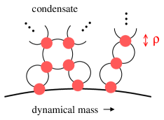
(a)	(b)

Figure 1: (a) Dynamical chiral symmetry breaking in QCD. The red blobs indicate non–perturbative interactions with a characteristic range $\rho\sim 0.3\,\textrm{fm}$. (b) Schematic illustration of the dynamical scales governing the valence and sea quark transverse momentum distributions at a low scale.[5]

3 Dynamical model based on chiral symmetry breaking

The qualitative difference between the valence and sea quark transverse momentum distributions can be illustrated[5] in a model of the nucleon that implements the effective low–energy dynamics resulting from chiral symmetry–breaking in QCD.[9] It uses “constituent” quarks/antiquarks with a dynamical mass $M\sim 0.3-0.4\,\textrm{GeV}$ as effective degrees of freedom below the chiral symmetry–breaking scale. The dynamical mass is accompanied by a coupling to a chiral field describing the long–wavelength phase fluctuations of the chiral condensate (Goldstone bosons, see Fig. 2a). The effective coupling constant is $M/F_{\pi}\sim$ 3–4, so that the dynamical system is strongly coupled and has to be solved non–perturbatively using the $1/N_{c}$ expansion. The effective dynamics applies to momenta up to the chiral symmetry breaking scale $\rho^{-2}$, which acts as an ultraviolet cutoff of the model.

Figure 2: Chiral quark–soliton model of the nucleon. (a) Effective dynamics. The quarks acquire a dynamical mass, accompanied by the coupling to a chiral field. (b) Nucleon solution in the large–$N_{c}$ limit. The classical chiral field (soliton) binds the valence quarks and creates quark–antiquark pairs.

The nucleon in the effective model develops a classical chiral field; in the rest frame it is of a generalized spherical form (“hedgehog”) and has a characteristic radius $R\sim M^{-1}$. The classical chiral field acts in a dual way: it binds $N_{c}$ valence quarks in a discrete bound–state level and distorts the chiral condensate, amounting to the coherent creation of additional quark–antiquark pairs out of the vacuum (chiral quark–soliton model, or relativistic mean–field approximation, see Fig. 2b).[9] Because the dynamics is formulated as a field theory it guarantees completeness of the quark single–particle states and preserves the partonic sum rules and positivity conditions of QCD, in the sense of a parametric expansion based on the hierarchy $\rho^{-2}\gg M^{2}$. The model is therefore uniquely suited to describe the nucleon’s parton densities at a low scale, especially sea quark distributions.

The calculation of parton distributions in the chiral quark–soliton model has been described in detail in the literature.[10, 11] The quark and antiquark densities can be computed either as number densities of field quanta in the infinite–momentum frame, or as light–cone correlation functions of the fields in the rest frame; the two formulations are equivalent thanks to the relativistic invariance and completeness of the model dynamics.[11] The transverse momentum integrals extend up to values of the order of the chiral–symmetry breaking scale $\rho^{-2}$, so that the model describes the “intrinsic” transverse momentum distributions due to non–perturbative nucleon structure. The model does not include effects of final–state interactions.

The parton distributions calculated in the chiral quark–soliton model are the light–cone momentum distributions of effective degrees of freedom — constituent quarks and antiquarks, which are to be matched with QCD quarks, antiquarks and gluons at the chiral symmetry–breaking scale $\rho^{-2}$ (see Fig. 3a). The matching can be performed either on the basis of a “microscopic” derivation of the effective chiral model from QCD, such as the instanton vacuum model,[13, 14] or with the help of empirical parton densities obtained from fits to DIS data. In the simplest approximation the composite quarks and antiquarks are identified with the QCD quarks and antiquarks at the scale $\rho^{-2}$, and the gluon density is set to zero. Its accuracy can be judged from the fact that in empirical leading–order parton densities[15] at the scale $\mu_{\rm LO}^{2}=0.3\,\textrm{GeV}^{2}$ about $\sim 30\%$ of the nucleon’s light–cone momentum is carried by gluons. Of particular significance is that the model describes well[16] the observed flavor–nonsinglet unpolarized sea $f_{1}^{\bar{d}-\bar{u}}(x)\equiv\bar{d}(x)-\bar{u}(x)$,[17] which is expected to be much less sensitive to “matching” effects than the flavor–singlet distributions (see Fig. 3b). The model also predicts a large flavor–nonsinglet polarized sea,[10, 11] hints of which are seen in recent global QCD fits including semi–inclusive DIS data and the RHIC $W^{\pm}$ production data.[18]

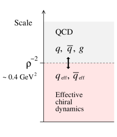
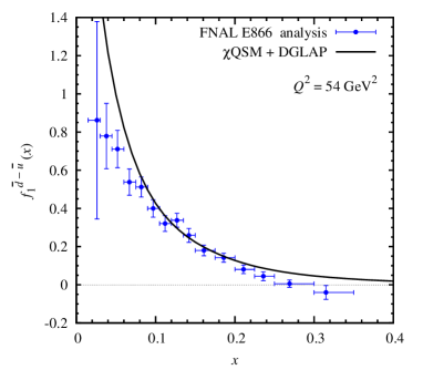
Figure 3: (a) Matching of the effective chiral model with QCD at the chiral symmetry–breaking scale $\rho^{-2}$. (b) Flavor–nonsinglet sea quark density in the chiral quark–soliton model,[16] after DGLAP evolution from the scale $\rho^{-2}$ to $Q^{2}=54\,\textrm{GeV}^{2}$, compared to the FNAL E866 Drell–Yan analysis.[17]

Figure 4a shows the intrinsic $p_{T}$ distributions of flavor–singlet unpolarized quarks at $x=0.1$ in the chiral quark–soliton model.[5] The valence quark distribution $f_{1}^{u+d-\bar{u}-\bar{d}}(x,p_{T})$ drops steeply with increasing $p_{T}$ and can roughly be approximated by a Gaussian shape. The average transverse momentum of the valence quarks is of the order $\langle p_{T}^{2}\rangle\sim M^{2}\sim R^{-2}$, corresponding to the inverse radius of the mean field binding the valence quarks (cf. Sec. 2 and Fig. 1b). The sea quark distribution $f_{1}^{\bar{u}+\bar{d}}(x,p_{T})$ extends up to much larger values of $p_{T}$. Closer inspection of the analytic expressions shows that it contains a “would–be” power–like tail of the form $f_{1}^{\bar{u}+\bar{d}}(x,p_{T})\sim C(x)/(p_{T}^{2}+M^{2})$, which is regulated by the UV cutoff representing the chiral symmetry–breaking scale $\rho^{-1}$. The coefficient $C(x)$ is determined by low–energy chiral dynamics at momenta of the order $M$ and model–independent. At $p_{T}\gg M$ the distributions exhibit some residual model dependence, due to choice of cutoff scheme implementing the chiral symmetry–breaking scale, which was studied numerically[5] and found to be minor up to $p_{T}\sim 3\,M\sim 1\,\textrm{GeV}$. These results clearly illustrate the qualitative difference between the valence and sea quark $p_{T}$ distributions due to dynamical chiral symmetry breaking. The features described here do not depend on the details of the model but rely only on the existence of two separate dynamical scales — the nucleon size $R$, and the chiral symmetry–breaking scale $\rho$.

file=f1_val_sea_area.eps,width=6.7cm	file=g1_val_sea_area.eps,width=6.7cm
(a)	(b)

Figure 4: (a) Intrinsic transverse momentum distributions of flavor–singlet unpolarized valence quarks $f_{1}^{u+d-\bar{u}-\bar{d}}$ (dashed line) and sea quarks $f_{1}^{\bar{u}+\bar{d}}$ (solid line) at $x=0.1$ in the chiral quark–soliton model.[5] The plot shows the radial distributions $2\pi p_{T}f_{1}(x,p_{T})$, so that the area under the curve corresponds to the $p_{T}$–integrated parton density in the model. The distributions and $p_{T}$ are given in units of the constituent quark mass $M=0.35\,\textrm{GeV}$. (b) Distributions of flavor–nonsinglet polarized valence quarks $g_{1}^{u-d-\bar{u}+\bar{d}}$ (dashed line) and sea quarks $g_{1}^{\bar{u}-\bar{d}}$ (solid line).

Similar behavior is found[5] in the transverse momentum distributions of flavor–nonsinglet polarized quarks, $g_{1}^{u-d-\bar{u}+\bar{d}}(x,p_{T})$ and $g_{1}^{\bar{u}-\bar{d}}(x,p_{T})$ (see Fig. 4b), which appear in the same order of the $1/N_{c}$ expansion as the flavor–singlet unpolarized distributions and share many features with them.[10, 11] The flavor–nonsinglet polarized sea quark distribution $g_{1}^{\bar{u}-\bar{d}}(x,p_{T})$ exhibits a would–be power–like tail of a form analogous to that of the flavor–singlet unpolarized distribution. The flavor–nonsinglet polarized valence quark distribution $g_{1}^{u-d-\bar{u}+\bar{d}}(x,p_{T})$ drops more rapidly at large $p_{T}$ than the flavor–singlet unpolarized one, making the discrepancy between sea and valence distributions at large $p_{T}\sim 1\,\textrm{GeV}$ even more pronounced than in the unpolarized case. We also note[5] that the unpolarized and polarized $p_{T}$ distributions in this model obey a general inequality (positivity condition) and reflect in a subtle manner the restoration of chiral symmetry at $p_{T}\sim\rho^{-1}$. An important practical question is how the “anomalously” large intrinsic $p_{T}$ of the flavor–singlet polarized sea affect the analysis of semi–inclusive DIS and $W^{\pm}$ production experiments aimed at extracting $g_{1}^{\bar{u}-\bar{d}}(x)\equiv\Delta\bar{u}(x)-\Delta\bar{d}(x)$, if such measurements are performed with a finite acceptance in $p_{T}$.

The chiral quark–soliton model also permits to evaluate the coordinate–space correlation functions,[5] the Fourier transforms of the TMD distributions entering in the coordinate–space CSS evolution equations.[2, 3, 4] Because the effective dynamics has a mass gap — the constituent quark mass $M$, the coordinate–space sea quark correlation function exhibits exponential behavior $\sim e^{-M\xi_{T}}$ over an intermediate range of distances $\rho\ll\xi_{T}\ll R$. At distances $\xi_{T}\sim R$ this behavior is modified by the spatial variation of the mean field; because $R\sim M^{-1}$ the window for a visible exponential dependence is actually rather small.

4 Experimental tests

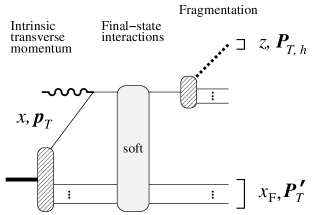
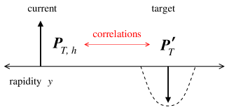
(a)	(b)

Figure 5: (a) Semi–inclusive DIS in QCD. The transverse momentum $P_{T,h}$ of hadrons in the current fragmentation region is compounded from the intrinsic $p_{T}$ of the parton, soft final–state interactions, and the transverse momentum of fragmentation process. (b) Hadron correlations between the current and target fragmentation regions.

The qualitative difference between the valence and sea quark $p_{T}$ distributions has numerous implications for semi–inclusive DIS measurements and could potentially be tested directly using special observables. In semi–inclusive DIS at $P_{T,h}\lesssim 1\,\textrm{GeV}$ the transverse momentum of the identified hadron $h$ is compounded from the intrinsic $p_{T}$ of the struck parton, soft QCD final–state interactions, and the transverse momentum incurred in the fragmentation process (see Fig. 5a). The strength of the different mechanisms is poorly known at present, making it difficult to quantify how differences in the intrinsic $p_{T}$ distributions express themselves in the observable hadron distributions. Differential measurements of kinematic dependencies (e.g. $z$ distributions for fixed $x$, $P_{T,h}$ distributions for fixed $z$) could help to disentangle the different mechanisms but require wide kinematic coverage and high statistics. Detailed measurements of multiplicities have recently been reported by the HERMES and COMPASS experiments.[19, 20] The valence quark region will be covered with high precision with the JLab 12 GeV Upgrade, but the kinematics is marginal for applying QCD factorization. A much broader kinematic region would become accessible with a future Electron–Ion Collider (EIC), permitting detailed studies of the production mechanism, $Q^{2}$–evolution, and sea quark distributions.[21, 22]

Special observables can detect systematic differences between the valence and sea quark $p_{T}$ distributions without detailed modeling of the semi–inclusive production mechanism.[5] One possibility is to measure the difference and sum of the charged pion multiplicity distributions for a deuteron target (isoscalar), which in schematic notation are proportional to

$$N_{\pi+,\;{\rm deut}}\;-\;N_{\pi-,\;{\rm deut}}\; \propto \;(e_{u}^{2}-e_{d}^{2})\;f_{1}^{u+d-\bar{u}-\bar{d}}\;\otimes\;D_{1}^{-},$$ (1)

$$N_{\pi+,\;{\rm deut}}\;+\;N_{\pi-,\;{\rm deut}}\; \propto \;(e_{u}^{2}+e_{d}^{2})\;f_{1}^{u+d+\bar{u}+\bar{d}}\;\otimes\;D_{1}^{+}.$$ (2)

Here $f_{1}^{q\mp\bar{q}}$ denote the difference/sum of the quark and antiquark distributions in the proton and $D_{1}^{\mp}=D_{1}^{u/\pi+}\mp D_{1}^{\bar{u}/\pi+}$ the difference/sum of the favored and unfavored pion fragmentation functions; isospin symmetry is used and the contribution of the strange sea has been neglected. A broader intrinsic $p_{T}$ distribution of sea quarks than of valence quarks should generally manifest itself in a decrease of the ratio $(N_{\pi+,\;{\rm deut}}-N_{\pi-,\;{\rm deut}})/(N_{\pi+,\;{\rm deut}}+N_{\pi+,\;{\rm deut}})$ with increasing pion transverse momentum $P_{T,\pi}$, or could simply be observed by comparing the normalized $P_{T,\pi}$ dependence of the difference and sum. Such measurements should be performed at moderately small values $x\sim 0.1$, where valence and sea quark densities are of comparable magnitude. Another possibility is to separate quarks and antiquarks in the target using charged kaons. $K^{+}$ are produced by favored fragmentation of $u$ quarks, whose distribution has both a valence and a sea component, while $K^{-}$ are produced from $\bar{u}$, which occurs in the sea only. Assuming identical transverse momentum distributions of strange quarks and antiquarks in the nucleon, $f_{1}^{s}=f_{1}^{\bar{s}}$, and neglecting differences in unfavored fragmentation, one expects the $K^{-}$ to have a broader $P_{T,K}$ distribution than the $K^{+}$.

An alternative experimental test of the different intrinsic $p_{T}$ distributions of valence and sea quarks would be comparing the transverse momentum distributions of dileptons (Drell–Yan pairs) produced in $pp$ and $\bar{p}p$ collisions. The pairs are produced in the annihilation of a quark and and antiquark from the two colliding hadrons. In $\bar{p}p$ collisions this is possible with valence quarks and antiquarks, while in $pp$ the sea is involved in at least one of the protons. We therefore expect a broader dilepton $P_{T,\,l+l-}$ distribution in $pp$ than in $\bar{p}p$ in the same kinematics. Again, such measurements would be most instructive at quark/antiquark momentum fractions $x_{1,2}\sim 0.1$, where valence and sea quark densities are of comparable magnitude.

Much more insight could be gained from measurements of hadron correlations between the current and the target fragmentation regions of semi–inclusive DIS (see Fig. 5b).[5] Such measurements could unravel the semi–inclusive production mechanism by answering the question what “balances” the observed $P_{T,h}$ of hadrons in the current fragmentation region — other current fragments, central rapidity hadrons, or target fragments. They could discriminate between scattering from sea and valence quarks by providing information on the hadronic products of the remnant system (charge, flavor, multiplicities). Under certain conditions they could even reveal the non–perturbative short–range correlations between sea quarks induced by chiral symmetry breaking. This would require a rapidity interval $\Delta y\gtrsim 4$ for clean separation of the current and target regions, moderate scales $Q^{2}\sim\textrm{few GeV}^{2}$ to avoid pQCD radiation, and access to quark/antiquark momentum fractions $x\sim 0.1$ where the non–perturbative sea is large; these conditions could be met in a “window” of moderate $\gamma^{\ast}N$ center–of–mass energies $W^{2}\sim 30\,\textrm{GeV}^{2}$. Such measurements could ideally be performed with a medium–energy EIC with appropriate forward hadron detection capabilities.[21]
Notice: Authored by Jefferson Science Associates, LLC under U.S. DOE Contract No. DE-AC05-06OR23177. The U.S. Government retains a non–exclusive, paid–up, irrevocable, world–wide license to publish or reproduce this manuscript for U.S. Government purposes.

References

- [1] J. C. Collins, D. E. Soper and G. Sterman, Nucl. Phys. B 250, 199 (1985).
- [2] For a recent review, see: J. Collins, these proceedings, arXiv:1307.2920 [hep-ph].
- [3] S. M. Aybat and T. C. Rogers, Phys. Rev. D 83, 114042 (2011).
- [4] P. Sun and F. Yuan, arXiv:1308.5003 [hep-ph].
- [5] P. Schweitzer, M. Strikman and C. Weiss, JHEP 1301, 163 (2013).
- [6] G. A. Miller, M. Strikman and C. Weiss, Phys. Rev. C 84, 045205 (2011).
- [7] P. Schweitzer, T. Teckentrup, A. Metz, Phys. Rev. D 81, 094019 (2010).
- [8] D. Diakonov, Prog. Part. Nucl. Phys. 51, 173 (2003).
- [9] D. Diakonov, V. Yu. Petrov and P. V. Pobylitsa, Nucl. Phys. B 306, 809 (1988).
- [10] D. Diakonov, V. Petrov, P. Pobylitsa, M. V. Polyakov and C. Weiss, Nucl. Phys. B 480, 341 (1996).
- [11] D. Diakonov, V. Petrov, P. Pobylitsa, M. Polyakov and C. Weiss, Phys. Rev. D 56, 4069 (1997).
- [12] X. Ji, arXiv:1305.1539 [hep-ph].
- [13] D. Diakonov, V. Yu. Petrov, Nucl. Phys. B 272, 457 (1986).
- [14] D. Diakonov, M. V. Polyakov and C. Weiss, Nucl. Phys. B 461, 539 (1996).
- [15] M. Gluck, P. Jimenez-Delgado and E. Reya, Eur. Phys. J. C 53, 355 (2008).
- [16] P. V. Pobylitsa, M. V. Polyakov, K. Goeke, T. Watabe and C. Weiss, Phys. Rev. D 59, 034024 (1999).
- [17] R. S. Towell et al. [FNAL E866/NuSea Collab.], Phys. Rev. D 64, 052002 (2001).
- [18] B. Surrow, presentation at QCD Evolution 2013, Jefferson Lab, May 6–10, 2013.
- [19] A. Airapetian et al. [HERMES Collaboration], Phys. Rev. D 87, 074029 (2013).
- [20] C. Adolph et al. [COMPASS Collaboration], arXiv:1305.7317 [hep-ex].
- [21] A. Accardi, V. Guzey, A. Prokudin and C. Weiss, Eur. Phys. J. A 48, 92 (2012).
- [22] A. Accardi, J. L. Albacete, M. Anselmino, N. Armesto, E. C. Aschenauer, A. Bacchetta, D. Boer and W. Brooks et al., arXiv:1212.1701 [nucl-ex].