Cosmological dependence of the measurements of luminosity function, projected clustering and galaxy-galaxy lensing signal

Abstract

Observables such as the luminosity function of galaxies, $\Phi(M)$, the projected clustering of galaxies, $w_{\rm p}(r_{\rm p})$, and the galaxy-galaxy lensing signal, $\Delta\Sigma$, are often measured from galaxy redshift surveys assuming a fiducial cosmological model for calculating distances to and between galaxies. There is a growing number of studies that perform joint analyses of these measurements and constrain cosmological parameters. We quantify the amount by which such measurements systematically vary as the fiducial cosmology used for the measurements is changed, and show that these effects can be significant at high redshifts ($z\sim 0.5$). We present a simple way that maps the measurements made using a particular fiducial cosmological model to any other cosmological model. Cosmological constraints (or halo occupation distribution constraints) that use the luminosity function, clustering measurements and galaxy-galaxy lensing signal but ignore these systematic effects may underestimate the confidence intervals on the inferred parameters.

1. Introduction

Large scale galaxy redshift surveys such as the Sloan digital Sky Survey (SDSS hereafter) have revolutionized the field of galaxy formation and cosmology. Data from such surveys has enabled precise measurements of the abundance of galaxies (see e.g., Blanton et al., 2003), the clustering of galaxies as a function of luminosity (see e.g., Zehavi et al., 2011) and the galaxy-galaxy lensing signal (see e.g., Sheldon et al., 2004; Mandelbaum et al., 2006, 2013). These measurements have been used to constrain an important outcome of the galaxy formation processes, the relation between galaxy luminosity (or stellar mass) and the underlying halo mass (Cacciato et al., 2009, 2013; Leauthaud et al., 2012; Tinker et al., 2013). It has also been argued that a joint analysis of these measurements can be used to constrain cosmological parameters, such as the matter density parameter and the amplitude of cosmological fluctuations using the data on small scales (see e.g., Seljak et al., 2005; Yoo et al., 2006; Cacciato et al., 2009; van den Bosch et al., 2013; More et al., 2013) and from large scales (Baldauf et al., 2010; Mandelbaum et al., 2013). Cosmological constraints have been obtained using the clustering of galaxies combined with other observables such as the mass-to-light ratio on cluster scales (van den Bosch et al., 2003; Tinker et al., 2005; van den Bosch et al., 2007), mass-to-number ratio (Tinker et al., 2012) or the galaxy-galaxy lensing signal (Cacciato et al., 2013; Mandelbaum et al., 2013).

To measure observables such as the luminosity function of galaxies, their projected clustering signal and the galaxy-galaxy lensing, the galaxy angular positions and redshifts are needed to be converted to cosmological distances between us and the galaxies and between galaxies themselves. These conversions are dependent upon the assumed cosmological model. It would be incorrect to assume that the measurements do not change when the cosmological model used to analyze the data is changed. Fitting analytical models to the same measurements with varying cosmological parameters can affect the constraints derived on the cosmological parameters.

The objective of this short letter is to quantify this effect for the particular set of observables, $\Phi(M)$, $w_{\rm p}(r_{\rm p})$ and $\Delta\Sigma$, and show that it is straightforward to account for such biases. In Section 2, we quantify analytically the sensitivity of each of these measurements to the assumed cosmological model. In Section 3, we use the example of the projected galaxy clustering signal to demonstrate that the effect on measurements of the changing reference model can be accounted for in a simple manner. In Section 4, we summarize and discuss our results.

2. Analytical estimates

2.1. Galaxy luminosity function

The abundance of galaxies is quantified by measurements of the luminosity function of galaxies, $\Phi(M){\rm d}M$, which gives the average number density of galaxies within the absolute magnitude range $M\pm{\rm d}M/2$. The luminosity functions are often determined from flux limited surveys and require us to convert the apparent magnitude $m$, of a galaxy into an absolute magnitude, and obtain the maximum distance out to which a galaxy with a given luminosity could have been observed given the flux limit of the survey. These conversions are dependent on the assumed cosmology in the following manner.

The apparent magnitude of a galaxy at redshift $z$ is related to the absolute magnitude via the distance modulus $\mu(z)=5.0\log(D_{\rm lum}[z,\Omega])+25$,

$$M=m-\mu(z)\,,$$ (1)

where $D_{\rm lum}(z,\Omega)$ is the luminosity distance (in units of $\>h^{-1}{\rm{Mpc}}$) in a particular cosmological model, $\Omega$. The maximum comoving distance, $\chi_{\rm max}$ to which this object can be observed given the magnitude limit $m_{\rm lim}$ of the survey is given by

$$\chi_{\rm max}=\frac{1}{1+z}10^{0.2(m_{\rm lim}-M-25)}$$ (2)

Thus differences in cosmology changes the luminosity of galaxies and the change in $\chi_{\rm max}$ affects the normalization of the luminosity function.

To estimate the amount by which the luminosity function can change due to a change in cosmological model, let us first assume that the luminosity function as a function of redshift changes extremely weakly within the survey area used to estimate it using some fiducial cosmological model . The luminosity function $\tilde{\Phi}(M,\tilde{\Omega})$, measured in some fiducial cosmological model $\tilde{\Omega}$ can be used to calculate the redshift dependence of the apparent magnitude counts $N(m,z){\rm d}m{\rm d}z$ per unit steradian, which is the observable in a true sense,

$$N(m,z){\rm d}m{\rm d}z=\tilde{\Phi}(m-\mu[z,\tilde{\Omega}]){\rm d}m\tilde{\chi}^{2}\frac{{\rm d}\tilde{\chi}}{{\rm d}z}{\rm d}z\,.$$ (3)

These number counts can be reinterpreted as a luminosity function in a cosmological model, $\Omega$ other than the fiducial model using the following equation,

$$\Phi(M,\Omega){\rm d}M = \frac{1}{V}\int_{0}^{z_{\rm max}}N(M+\mu[z,\Omega],\,z)\,{\rm d}M\,{\rm d}z$$

$$= \frac{1}{V}\int_{0}^{z_{\rm max}}\tilde{\Phi}(M+\mu[z,\Omega]-\mu[z,\tilde{\Omega}])\,{\rm d}M\,\tilde{\chi}^{2}\frac{{\rm d}\tilde{\chi}}{{\rm d}z}{\rm d}z.$$

Here, $z_{\rm max}$ denotes the maximum redshift to which a galaxy can be observed in the redshift survey, given its absolute magnitude in the cosmological model $\Omega$, and $V$ denotes the comoving volume encompassed by the Universe below this redshift. In Figure 1, we use the Schechter fit for the luminosity function provided by Blanton et al. 2003, in a $\Omega_{\rm m}=0.3$ model and show the residuals of the luminosity function in $\Omega_{\rm m}=0.25$ and $\Omega_{\rm m}=0.35$ models computed using the above equation. We have assumed the magnitude limit in $r$-band of $17.77$ corresponding to the spectroscopic sample in SDSS.

Although the measurement errors on the luminosity function are large, the difference is a systematic change in the shape of the luminosity function, and can be as large as $\sim 20$ percent at the bright end. Since the errorbars are difficult to propagate in an integral equation such as the one above, the ideal way is to change the prediction for a particular cosmological model to predict the counts in fiducial model used to obtain the luminosity function.

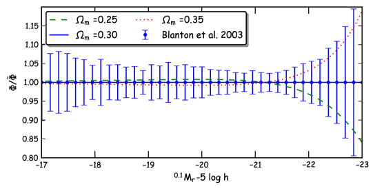
Figure 1.— The ratio of the SDSS luminosity function from Blanton et al. (2003) derived in a $\Omega_{\rm m}=0.3$ model with respect to the luminosity function expected if the data was analyzed using $\Omega_{\rm m}=0.25$ or $\Omega_{\rm m}=0.35$ model.

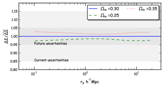
Figure 2.— The ratio of the galaxy-galaxy lensing signal around BOSS galaxies expected assuming an $\Omega_{\rm m}=0.3$ model with respect to that expected if the data was analyzed using $\Omega_{\rm m}=0.25$ or $\Omega_{\rm m}=0.35$ model. The light and dark grey band corresponds to current and future uncertainties.

2.2. Projected clustering measurement

For a flat $\Lambda$CDM model, the projected and the line-of-sight comoving separations between two galaxies separated in redshift by a small difference $\Delta z$ is given by,

$$r_{\rm p}=\chi(z_{\rm eff})\theta;\,\,\,\,\pi=\frac{c}{H_{0}\,E(z_{\rm eff})}\Delta z\,\,,$$ (6)

respectively, where $\chi(z_{\rm eff})$ is the comoving distance to the effective redshift $z_{\rm eff}$, $\theta$ denotes the angular separation of the two galaxies, $c$ denotes the speed of light, $H_{0}$ is the Hubble constant and $E(z)$ is the expansion function. Here we have ignored the finite redshift width of the galaxy sample and assumed a particular effective redshift to convert the angular positions and redshift into distances. These equations can then be used to count the number of pairs of galaxies at a given separation vector $(r_{\rm p},\pi)$, and compare it to the number of pairs expected if the galaxies were distributed in a random manner. The excess number of pairs over those expected in a random distribution gives the clustering signal at the effective redshift, $\xi(r_{\rm p},\pi)$. The projected clustering is then obtained by integrating $\xi(r_{\rm p},\pi)$ along the line-of-sight,

$$w_{\rm p}(r_{\rm p},z_{\rm eff}) = 2\int_{0}^{\pi_{\rm max}}\xi(r_{\rm p},\pi,z_{\rm eff}){\rm d}\pi\,,$$ (7)

$$= 2\int_{0}^{\Delta z_{\rm max}}\xi(r_{\rm p},\pi,z_{\rm eff})\frac{c}{H_{0}E(z_{\rm eff})}{\rm d}(\Delta z)\,.\vspace{0.1cm}$$ (8)

In addition to changing slightly the composition of galaxy samples, there are three different ways a change in the cosmology will affect the $w_{\rm p}$ measurements. If a cosmology other than the fiducial is used to analyze the data, then a given angular scale corresponds to a different comoving projected separation scale. This difference can be small at low redshift (see e.g. Zehavi et al., 2011, $\sim 1$ percent due to a change in $\Omega_{\rm m}$ from 0.25 to 0.3 at $z=0.15$). As $w_{\rm p}\propto r_{\rm p}^{-1}$, the change in projected separation scale roughly corresponds to a similar change in the value of $w_{\rm p}(r_{\rm p})$ when the cosmology is changed.

The second effect is due to change in the factor $E(z)$ as cosmology is changed, and this changes the value of $w_{\rm p}(r_{\rm p})$ by a multiplicative constant at all scales. This effect is important, especially at higher redshift (at $z\sim 0.5$, the difference in the expansion functions is $3.5$ per cent between $\Omega_{\rm m}$ of 0.25 and 0.3). Such effects due to the change of transverse (and line-of-sight) scales are usually taken into account when analysing baryon acoustic oscillations (see e.g., Blake & Glazebrook, 2003; Eisenstein et al., 2005; Percival et al., 2007; Anderson et al., 2012) and redshift space distortions (see e.g., Ballinger et al., 1996; Tegmark et al., 2006; Blake et al., 2011).

The third effect on $w_{\rm p}(r_{\rm p})$ is subtle and is related to the change in the integration limit in the above equation, as a given value of $\pi_{\rm max}$ corresponds to a different value of $\Delta z_{\rm max}$. For sufficiently large values of $\pi_{\rm max}$ as are employed in observations (typically $60\sim 100\>h^{-1}{\rm{Mpc}}$) this effect is quite small as the value of $\xi(r_{\rm p},\pi)$ at large values of $\pi$ does not dominate the $w_{\rm p}(r_{\rm p})$ integral. Note however, that even this small difference can be easily accounted for by adopting a different $\pi_{\rm max}$ value when computing the analytical prediction.

In Table 1, we present the ratios of the comoving distance and the expansion function for three different cosmological models, at different redshifts. The range of cosmological models is chosen to be such that it is well within the ranges of cosmological constraints obtained by a number of joint analyses involving the clustering measurement. The fractions $f^{\Omega_{\rm m}=0.30}_{E(z)}$ and $f^{\Omega_{\rm m}=0.30}_{\chi(z)}$ are defined in the caption, and are chosen such that they roughly correspond to the deviations in the clustering signal expected when the data is analysed in two different cosmologies. The two effects change the clustering signal in the same direction.

It can be seen that the combination of the first two effects are small $\sim 2$ per cent differences between $\Omega_{\rm m}=0.25$ and $\Omega_{\rm m}=0.35$ models (although are systematically in the same direction on all scales) for low redshift ($z\sim 0.1$) analyses. At $z\sim 0.5$, the effects cause $\sim 10$ percent differences between the two cosmological models above and can be very important given the statistical errors in the measurements of $w_{\rm p}(r_{\rm p})$ with current and upcoming large surveys.

Table 1Cosmological dependence of comoving distance and the expansion function

Redshift	$\Omega_{\rm m}$	$f^{\Omega_{\rm m}=0.3}_{\chi(z)}$	$f^{\Omega_{\rm m}=0.3}_{E(z)}$
0.1	0.25	0.996	0.992
0.1	0.30	1.000	1.000
0.1	0.35	1.004	1.007
0.3	0.25	0.989	0.978
0.3	0.30	1.000	1.000
0.3	0.35	1.011	1.022
0.5	0.25	0.982	0.965
0.5	0.30	1.000	1.000
0.5	0.35	1.017	1.034

The fraction $f^{\Omega_{\rm m}=0.30}_{E(z)}$ is defined as the ratio of the expansion function in a given cosmology to that in $\Omega_{\rm m}=0.30$ cosmology, i.e., $E(z,\Omega_{\rm m})/E(z,\Omega_{\rm m}=0.30)$. The fraction $f^{\Omega_{\rm m}=0.30}_{\chi(z)}$ is defined as the ratio of the comoving distance in $\Omega_{\rm m}=0.30$ cosmology, to that in another cosmology i.e., $\chi(z,\Omega_{\rm m}=0.30)/\chi(z,\Omega_{\rm m})$.

Table 2Cosmological dependence of comoving distance and the critical density

$z_{\rm l}$	$z_{\rm s}$	$\Omega_{\rm m}$	$f^{\Omega_{\rm m}=0.3}_{\chi(z_{\rm l})}$	$f^{\Omega_{\rm m}=0.3}_{\Sigma_{\rm crit}(z_{\rm l},z_{\rm s})}$
0.1	0.5	0.25	0.996	1.0077
0.1	0.5	0.30	1.000	1.0000
0.1	0.5	0.35	1.004	0.9925
0.1	0.7	0.25	0.996	1.0077
0.1	0.7	0.30	1.000	1.0000
0.1	0.7	0.35	1.004	0.9926
0.1	0.9	0.25	0.996	1.0077
0.1	0.9	0.30	1.000	1.0000
0.1	0.9	0.35	1.004	0.9926
0.5	0.8	0.25	0.982	1.0362
0.5	0.8	0.30	1.000	1.0000
0.5	0.8	0.35	1.017	0.9676
0.5	1.0	0.25	0.982	1.0358
0.5	1.0	0.30	1.000	1.0000
0.5	1.0	0.35	1.017	0.9680
0.5	2.0	0.25	0.982	1.0341
0.5	2.0	0.30	1.000	1.0000
0.5	2.0	0.35	1.017	0.9698

The fraction $f^{\Omega_{\rm m}=0.30}_{\chi(z)}$ is defined the same way as in Table 1. The fraction $f^{\Omega_{\rm m}=0.30}_{\Sigma_{\rm crit}(z_{\rm l},z_{\rm s})}$ is defined as the ratio of the critical surface density in the $\Omega_{\rm m}=0.30$ model to that in another cosmology, i.e., $f^{\Omega_{\rm m}=0.30}_{\Sigma_{\rm crit}(z_{\rm l},z_{\rm s})}={\Sigma_{\rm crit}(z_{\rm l},z_{\rm s},\Omega_{\rm m}=0.30)}/{\Sigma_{\rm crit}(z_{\rm l},z_{\rm s},\Omega_{\rm m})}$.

2.3. Galaxy-galaxy lensing measurement

The primary observable for the galaxy-galaxy lensing signal is the tangential ellipticity of background galaxies in the vicinity of foreground galaxies. The galaxy-galaxy lensing signal is often reported as the excess surface density, $\Delta\Sigma$ by averaging the tangential component of ellipticity around an ensemble of galaxies

$$\Delta\Sigma(r_{\rm p})=\tilde{\Sigma}_{\rm crit}(z_{\rm l},z_{\rm s})\langle\epsilon\rangle(r_{\rm p})\,,$$ (9)

where $r_{\rm p}$ denotes the projected comoving separation $r_{\rm p}$ between the two galaxies at the redshift of the foreground lens, and $\Sigma_{\rm crit}(z_{\rm l},z_{\rm s})$ is a cosmology dependent factor called the critical surface density which is defined as

$$\Sigma_{\rm crit}(z_{\rm l},z_{\rm s})=\frac{c^{2}}{4\pi G}\frac{D_{\rm A}(z_{\rm s})(1+z_{\rm l})^{-2}}{D_{\rm A}(z_{\rm l},z_{\rm s})D_{\rm A}(z_{\rm l})}\,.$$ (10)

Here $D_{\rm A}(z_{\rm l})$, $D_{\rm A}(z_{\rm s})$ and $D_{\rm A}(z_{\rm l},z_{\rm s})$ are the angular diameter distances to the lens, the source, and between the lens and source, respectively, and the $(1+z_{\rm l})^{-2}$ factor arises from the use of comoving units.

The cosmology dependence enters the measurement of $\Delta\Sigma$ in two ways. The first one is similar to that discussed in the previous subsection. A given angular scale on the sky corresponds to different comoving projected scales in different cosmological models. Since the excess surface density is also roughly proportional to $r_{\rm p}^{-1}$, the percentage change in $\Delta\Sigma$ is similar to the percentage in the comoving distances. The second effect leads to a change in the normalization of $\Delta\Sigma$ due to the dependence of $\Sigma_{\rm crit}$ on the cosmological parameters and depends upon both the source and lens redshift distribution.

In Table 2, we calculate the ratios of the comoving distance and the critical surface density for three different cosmological models and for different combinations of source and lens redshifts, to quantify the effect it can have on the galaxy-galaxy lensing signal. The fraction $f^{\Omega_{\rm m}=0.30}_{\Sigma_{\rm crit}(z_{\rm l},z_{\rm s})}$ is defined as the ratio of the critical surface density in a cosmological model to that in the $\Omega_{\rm m}=0.30$ model. The two effects go in opposite direction making the lensing signal less sensitive to the cosmological parameters than the clustering signal, and even though the current statistical errors are large, these systematic dependence of the lensing signal on the fiducial cosmology can be also seen in real data (Miyatake et al., in preparation).

Ideally to account for the cosmological dependence of this signal, one needs to also consider both the source and lens redshift distributions. However if the lens redshift range is narrow enough, one can assume the lenses to be located at a similar effective redshift, $z_{\rm eff}$. In addition, note that $f^{\Omega_{\rm m}=0.30}_{\Sigma_{\rm crit}(z_{\rm l},z_{\rm s})}$ for same lens redshift and the same cosmology is a very weakly varying function of source redshift (see Table 2). This implies that the amplitude correction can be safely assumed to be a constant normalization shift fairly independent of the source redshift distribution. This correction can then be calculated at the median redshift of the source galaxy population and applied to the model before comparing to data. In Fig. 2, we compare the differences in $\Delta\Sigma$ expected due to change in the fiducial cosmological model expected from these corrections at $z\sim 0.5$ and find that the deviations can be of the order of $4-5$ percent between $\Omega_{\rm m}=0.25$ and $\Omega_{\rm m}=0.35$ models. Although small compared to errors possible with existing data, it is important to note, that they systematically go in the opposite direction as the clustering signal. The errors are expected to go down to $5$ percent or better with upcoming surveys such as the Hyper Suprime-Cam survey.

3. Tests on real data for the projected clustering function

We now use galaxies from the SDSS-III Baryon Oscillation Spectroscopic Survey project Data Release 9 (hereafter BOSS; Dawson et al., 2013; Ahn et al., 2012), and demonstrate for the case of the projected clustering measurement how well the effects mentioned in the Section 2.2 capture the relevant changes to the measurement. We analyze the projected clustering using three different cosmological models and show that they differ by the amount expected from the discussion in the previous section. We choose all galaxies in the northern region of BOSS with redshifts between $z\in[0.47,0.59]$ and $M_{*}>10^{10.2}\>{\rm M_{\odot}}$ where $M_{*}$ denotes the stellar mass calculated using the stellar population synthesis models by the Portsmouth group (Maraston et al., 2012). This yields a crude and approximate volume limited sample of galaxies (More et al., in preparation), however this particular aspect is not relevant to the results presented here. The effective redshift of the sample is $z_{\rm eff}=0.53$.

In the top panel of Figure 3, we show the clustering of galaxies measured by assuming three different flat $\Lambda$CDM cosmological models with varying $\Omega_{\rm m}$ while converting the angular positions and redshifts to distances. The solid circles in the lower panel denote the differences between the measured clustering signal in a given cosmological model to that in the $\Omega_{\rm m}=0.30$ model. The measurement errorbars are small enough that the differences between the cosmological models are larger than the statistical error and are systematic in nature. Fitting a constant to the (inverse variance-weighted) residuals results in $0.062\pm 0.005\,(-0.042\pm 0.003)$ for the $\Omega_{\rm m}=0.25\,(0.35)$ model.

Next we take the measurements in the $\Omega_{\rm m}=0.25$ model, and predict the clustering expected in the $\Omega_{\rm m}=0.30$ model as follows. To account for the first effect discussed in Section 2.2, we change the projected comoving scale of the measurement from the $\Omega_{\rm m}=0.25$ analysis to

$$r_{\rm p}^{\rm corr}=r_{\rm p}(\Omega_{\rm m}=0.25)\frac{\chi(z_{\rm eff},\Omega_{\rm m}=0.30)}{\chi(z_{\rm eff},\Omega_{\rm m}=0.25)}\,.$$ (11)

In addition we also change the amplitude of $w_{\rm p}$ such that

$$w_{\rm p}^{\rm corr}=w_{\rm p}(\Omega_{\rm m}=0.25)\frac{E(z_{\rm eff},\Omega_{\rm m}=0.25)}{E(z_{\rm eff},\Omega_{\rm m}=0.30)}\,.\vspace{0.1cm}$$ (12)

We also use similar corrections to the clustering measurements in the $\Omega_{\rm m}=0.35$ model to deduce the clustering measurements in the $\Omega_{\rm m}=0.30$ model. The filled triangles in the bottom panel of Figure 3 show the difference between these corrected clustering measurement and the projected clustering measurement in the $\Omega_{\rm m}=0.30$ model using filled triangles (the green [red] triangles correspond to the $\Omega_{\rm m}=0.25\,[0.35]$ model corrected to that in $\Omega_{\rm m}=0.30$). We see that this recovers the clustering measurement very accurately. A constant model fit to the residuals now gives $0.004\pm 0.005\,(0.005\pm 0.004)$ for the $\Omega_{\rm m}=0.25\,(0.35)$ model and the residuals no longer have either just positive or negative sign.

Although in our case, we have corrected the data for the cosmological dependence, in modelling applications, it is better to account for the differences in the model itself. Errors, typically done using a jack-knife estimator (with regions of equal areal coverage), will not depend upon the cosmological model. But errors obtained using covariances with mock simulations populated with galaxies, may require a revision too. Exploring these details is beyond the scope of this short letter.

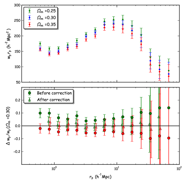
Figure 3.— The projected clustering (shown as $w_{\rm p}\,r_{\rm p}$ to reduce the dynamical scale) of an approximately volume limited subsample of CMASS galaxies, analyzed using different flat $\Lambda$CDM cosmological models are shown in the top panel with symbols of different colors. The clustering when the data is analyzed with $\Omega_{\rm m}=0.25\,(0.35)$ is the largest (smallest). The solid circles in the bottom panel show the difference between the measurements with respect to the measurements in the $\Omega_{\rm m}=0.30$ model. Accounting for the effects discussed in Section 2, we can use the measurements performed using $\Omega_{\rm m}=0.25$ or $\Omega_{\rm m}=0.35$ model and accurately recover the measurements in the $\Omega_{\rm m}=0.30$ model. The differences between these corrected measurements and the clustering in the $\Omega_{\rm m}=0.30$ model are shown using filled triangles. There is a small offset added in the x-direction in the lower panel for clarity.

4. Summary

We have presented analytical estimates for the cosmological dependence of the galaxy luminosity function, $\Phi(M)$, the projected clustering measurement, $w_{\rm p}(r_{\rm p})$, and the galaxy-galaxy lensing signal $\Delta\Sigma$ obtained from a galaxy redshift survey. We showed that these measurements change in different cosmological models due to the difference in the comoving distances, $\chi(z)$, the expansion functions, $E(z)$, and the change to the critical surface density between lens and source galaxies used to measure the lensing signal.

These changes are small for low redshift surveys such as SDSS-I, but given the systematic nature of the shifts can bias the cosmological constraints obtained from a joint analysis of $\Phi(M)$, $w_{\rm p}(r_{\rm p})$ and $\Delta\Sigma$. These systematic effects can be very important at higher redshifts which use these observables and for ongoing and future surveys which can measure these observables with ever-increasing precision. Performing a cosmological analysis with these observables requires one to account for the cosmological parameter dependence of the observables themselves. We have presented an analytical framework to change the predictions for a particular cosmological model to the ones in the fiducial cosmological model, thus allowing a fair comparison between the model and the data.

We tested the framework for the specific case of the projected clustering measurement $w_{\rm p}(r_{\rm p})$ using existing data from the SDSS-BOSS survey. We analyzed this data in the context of three different flat $\Lambda$CDM cosmological models. We found that the differences in the measurements are systematic in nature and significant given the errorbars. We also found that the nature of these differences is of the same magnitude as that predicted from the analytical framework, and hence can be easily accounted for.

If a cosmological analysis is run without accounting for these systematic issues, one runs the risk of biasing the cosmological parameters to values close to the ones assumed in the fiducial cosmology used to carry out the measurements, and significantly underestimate the errors. In future work, we plan to quantify how the recent cosmological constraints obtained using joint fits to abundance, clustering and lensing of galaxies by Cacciato et al. (2013) may be affected due to these systematic issues. We also plan to investigate the effects of these systematics on the joint analysis of clustering and lensing on large scales in Mandelbaum et al. (2013), especially for the high redshift sample.

References

- Ahn et al. (2012) Ahn, C. P., et al. 2012, ApJS, 203, 21
- Anderson et al. (2012) Anderson, L., et al. 2012, MNRAS, 427, 3435
- Baldauf et al. (2010) Baldauf, T., Smith, R. E., Seljak, U., & Mandelbaum, R. 2010, Phys. Rev. D, 81, 063531
- Ballinger et al. (1996) Ballinger, W. E., Peacock, J. A., & Heavens, A. F. 1996, MNRAS, 282, 877
- Blake & Glazebrook (2003) Blake, C., & Glazebrook, K. 2003, ApJ, 594, 665
- Blake et al. (2011) Blake, C., et al. 2011, MNRAS, 418, 1725
- Blanton et al. (2003) Blanton, M. R., et al. 2003, ApJ, 592, 819
- Cacciato et al. (2009) Cacciato, M., van den Bosch, F. C., More, S., Li, R., Mo, H. J., & Yang, X. 2009, MNRAS, 394, 929
- Cacciato et al. (2013) Cacciato, M., van den Bosch, F. C., More, S., Mo, H., & Yang, X. 2013, MNRAS, 430, 767
- Dawson et al. (2013) Dawson, K. S., et al. 2013, AJ, 145, 10
- Eisenstein et al. (2005) Eisenstein, D. J., et al. 2005, ApJ, 633, 560
- Leauthaud et al. (2012) Leauthaud, A., et al. 2012, ApJ, 744, 159
- Mandelbaum et al. (2006) Mandelbaum, R., Seljak, U., Kauffmann, G., Hirata, C. M., & Brinkmann, J. 2006, MNRAS, 368, 715
- Mandelbaum et al. (2013) Mandelbaum, R., Slosar, A., Baldauf, T., Seljak, U., Hirata, C. M., Nakajima, R., Reyes, R., & Smith, R. E. 2013, MNRAS, 432, 1544
- Maraston et al. (2012) Maraston, C., et al. 2012, ArXiv e-prints
- More et al. (2013) More, S., van den Bosch, F. C., Cacciato, M., More, A., Mo, H., & Yang, X. 2013, MNRAS, 430, 747
- Percival et al. (2007) Percival, W. J., Cole, S., Eisenstein, D. J., Nichol, R. C., Peacock, J. A., Pope, A. C., & Szalay, A. S. 2007, MNRAS, 381, 1053
- Seljak et al. (2005) Seljak, U., et al. 2005, Phys. Rev. D, 71, 043511
- Sheldon et al. (2004) Sheldon, E. S., et al. 2004, AJ, 127, 2544
- Tegmark et al. (2006) Tegmark, M., et al. 2006, Phys. Rev. D, 74, 123507
- Tinker et al. (2013) Tinker, J. L., Leauthaud, A., Bundy, K., George, M. R., Behroozi, P., Massey, R., Rhodes, J., & Wechsler, R. 2013, ArXiv e-prints
- Tinker et al. (2005) Tinker, J. L., Weinberg, D. H., Zheng, Z., & Zehavi, I. 2005, ApJ, 631, 41
- Tinker et al. (2012) Tinker, J. L., et al. 2012, ApJ, 745, 16
- van den Bosch et al. (2003) van den Bosch, F. C., Mo, H. J., & Yang, X. 2003, MNRAS, 345, 923
- van den Bosch et al. (2013) van den Bosch, F. C., More, S., Cacciato, M., Mo, H., & Yang, X. 2013, MNRAS, 430, 725
- van den Bosch et al. (2007) van den Bosch, F. C., et al. 2007, MNRAS, 376, 841
- Yoo et al. (2006) Yoo, J., Tinker, J. L., Weinberg, D. H., Zheng, Z., Katz, N., & Davé, R. 2006, ApJ, 652, 26
- Zehavi et al. (2011) Zehavi, I., et al. 2011, ApJ, 736, 59