Galaxy mergers on a moving mesh: a comparison with smoothed-particle hydrodynamics

Abstract

Galaxy mergers have been investigated for decades using smoothed particle hydrodynamics (SPH), but recent work highlighting inaccuracies inherent in the traditional SPH technique calls into question the reliability of previous studies. We explore this issue by comparing a suite of gadget-3 SPH simulations of idealised (i.e., non-cosmological) isolated discs and galaxy mergers with otherwise identical calculations performed using the moving-mesh code arepo. When black hole (BH) accretion and active galactic nucleus (AGN) feedback are not included, the star formation histories (SFHs) obtained from the two codes agree well. When BHs are included, the code- and resolution-dependent variations in the SFHs are more significant, but the agreement is still good, and the stellar mass formed over the course of a simulation is robust to variations in the numerical method. During a merger, the gas morphology and phase structure are initially similar prior to the starburst phase. However, once a hot gaseous halo has formed from shock heating and AGN feedback (when included), the agreement is less good. In particular, during the post-starburst phase, the SPH simulations feature more prominent hot gaseous haloes and spurious clumps, whereas with arepo, gas clumps and filaments are less apparent and the hot halo gas can cool more efficiently. We discuss the origin of these differences and explain why the SPH technique yields trustworthy results for some applications (such as the idealised isolated disc and galaxy merger simulations presented here) but not others (e.g., gas flows onto galaxies in cosmological hydrodynamical simulations).

1 Introduction

Galaxy mergers are a natural and crucial ingredient of the $\Lambda$CDM hierarchical galaxy formation paradigm. Although the fraction of galaxies undergoing a merger at any given time is relatively small, nearly all galaxies will experience a merger at some point in their histories (e.g., Stewart et al., 2009; Lotz et al., 2011; López-Sanjuan et al., 2013). Particularly significant are ‘major’ mergers, which can be transformative. In these cases, mergers violently alter the orbits of the stars in the galaxies and can transform rotationally supported discs into dispersion-supported spheroids (e.g., Toomre & Toomre, 1972; Toomre, 1974; Barnes, 1988, 1992; Hernquist, 1992, 1993; Cox et al., 2006b). Furthermore, tidal torques exerted by the galaxies upon one another drive gas inwards (e.g., Barnes & Hernquist, 1991, 1996), thereby resulting in powerful starbursts (e.g., Mihos & Hernquist, 1994b, 1996), triggering active galactic nuclei (AGN) (e.g., Di Matteo et al., 2005), altering metallicity gradients (Kobayashi, 2004; Di Matteo et al., 2009b; Rupke et al., 2010; Torrey et al., 2012a), and leaving behind signatures of the starbursts and AGN activity in the form of compact stellar cores (e.g., Mihos & Hernquist, 1994a; Hopkins et al., 2008) and supermassive black holes (BHs; e.g., Hopkins et al., 2007). Also, mergers may drive the size evolution of quiescent galaxies (e.g., Buitrago et al., 2008; Lani et al., 2013). It has thus been proposed that various seemingly different observational classes of objects in the Universe – including blue star-forming disc galaxies, irregular galaxies of a variety of morphologies, heavily dust-obscured (ultra-)luminous infrared galaxies ((U)LIRGs), both obscured and unobscured AGN, ‘post-starburst’ (aka ‘K+A’) galaxies, and ‘red and dead’ elliptical galaxies – may be related in a merger-driven evolutionary sequence (e.g., Sanders et al., 1988a, b; Sanders & Mirabel, 1996; Springel et al., 2005a; Hopkins et al., 2006; Snyder et al., 2011).

Galaxy mergers have been studied using numerical simulations for more than forty years (Toomre & Toomre 1972; Toomre 1974; Kozlov et al. 1974a, b), and for more than seventy years if one considers the pioneering laboratory method of Holmberg (1941). Although the early simulations included only gravity, they provided much insight into the effects of mergers on galaxy morphologies, the formation of tidal tails and shells, and the kinematics of merger remnants. More sophisticated simulations (e.g., Hernquist, 1989; Barnes & Hernquist, 1991, 1996; Mihos & Hernquist, 1994a, 1996) included also gas dynamical processes, which can be important for many galaxies because a significant fraction of the baryonic mass is in gas, and, unlike the stars, the gas is dissipational. Hydrodynamic simulations of galaxy mergers have helped us to understand the driving mechanism of starbursts (e.g., Hernquist, 1989; Barnes & Hernquist, 1991; Mihos & Hernquist, 1996; Di Matteo et al., 2007, 2008; Cox et al., 2008), supermassive BH fueling and feedback (e.g., Di Matteo et al., 2005; Springel et al., 2005b; Kazantzidis et al., 2005; Robertson et al., 2006b; Johansson et al., 2009; Mayer et al., 2010; Hopkins et al., 2012), feedback from supernovae (e.g., Cox et al., 2006c), the kinematics of merger remnants (e.g., Bendo & Barnes 2000; Naab & Burkert 2003; Naab, Jesseit, & Burkert 2006a, b; Bournaud et al. 2005; Cox et al. 2006b; Di Matteo et al. 2009a; Bois et al. 2010, 2011), the survivability of discs during mergers (e.g., Barnes, 2002; Springel & Hernquist, 2005; Robertson et al., 2006a; Robertson & Bullock, 2008; Hopkins et al., 2009; Puech et al., 2012), the sizes of merger remnants (e.g., Bournaud et al. 2007; Naab, Johansson, & Ostriker 2009; Wuyts et al. 2010; Hilz et al. 2013; Perret et al. 2013), and the formation of local (e.g., Younger et al., 2009) and high-redshift ULIRGs (e.g., Narayanan et al., 2009, 2010a, 2010b; Hayward et al., 2011, 2012, 2013; Karl et al., 2013; Snyder et al., 2013), among many other topics.

Whereas cosmological simulations are routinely performed using both grid-based Eulerian and particle-based pseudo-Lagrangian methods, idealised isolated (i.e., non-cosmological) galaxy merger simulations have almost always been performed using pseudo-Lagrangian smoothed particle hydrodynamics (SPH; Lucy 1977; Gingold & Monaghan 1977; see Rosswog 2009, Springel 2010b, and Price 2012 for recent reviews). SPH is well-suited to simulating galaxy mergers because it naturally treats the large bulk velocities present before the discs coalesce and it concentrates resolution elements in regions where the mass is located (the galaxy centre(s); see section 9.4 of Springel 2010a for further discussion). Furthermore, the other primary method used for galaxy formation studies, adaptive mesh refinement (AMR), does not treat self-gravity as accurately as particle-based approaches (O’Shea et al., 2005; Heitmann et al., 2008). For these reasons, relatively few galaxy merger simulations have been performed using AMR (to our knowledge, the only published examples of such simulations are Kim et al. 2009; Teyssier et al. 2010; Bournaud et al. 2011; Chapon et al. 2013; Perret et al. 2013; Powell et al. 2013).

Recent studies that used simple, idealised test problems and cosmological simulations have highlighted potentially significant problems that are inherent in the standard formulation of the SPH technique. Agertz et al. (2007) demonstrated that the standard implementation of SPH artificially suppresses the Kelvin–Helmholtz (KH) and Raleigh–Taylor (RT) instabilities because the method introduces spurious pressure forces near steep density gradients that allow a gap to be created between particles, thereby reducing their interactions. Furthermore, SPH can artificially damp subsonic turbulence (Bauer & Springel, 2012) and restricts gas stripping from substructures falling on to haloes (Sijacki et al., 2012). However, fixed grid-based methods also have drawbacks; for example, these codes are not Galilean invariant and can produce over-mixing (Springel, 2010a).

Partially motivated by the limitations inherent in the traditional SPH technique, Springel (2010a) developed a novel moving-mesh hydrodynamics code known as arepo. Although similar approaches have been proposed earlier, such techniques have not yet seen wide-spread use in astrophysical applications. arepo is quasi-Lagrangian because the unstructured mesh is advected with the flow. Whereas the motion of the grid reduces mass exchange between cells compared with a static mesh (e.g., Genel et al., 2013), arepo is not strictly Lagrangian because the mass in a given cell can change with time. Nevertheless, arepo offers a number of advantages over other methods that make it attractive for astrophysical applications. For example, it is Galilean invariant and naturally concentrates resolution elements in dense regions, similar to particle-based techniques. Because arepo uses a finite-volume method to solve the Euler equations, it is better than traditional SPH at capturing shocks and contact discontinuities and does not artificially suppress fluid instabilities (see also Bauer & Springel, 2012; Sijacki et al., 2012). Its ability to better capture weak shocks than SPH is potentially significant for cosmological problems because these features are ubiquitous in the cosmic web (e.g., Keshet et al., 2003). Because of its hybrid nature, arepo performs better than (or at least as well as) both traditional SPH and grid-based approaches for idealised test problems. Thus, it is useful to compare the results of arepo simulations to those of simulations performed using other techniques to investigate what effects, if any, the shortcomings of the traditional methods have on the results of cosmological and idealised galaxy merger simulations.

Some comparisons between cosmological simulations performed with arepo and gadget-3 – in which all other ingredients, including the gravity solver and sub-resolution models, are identical – have already been made. In some situations, the baryonic properties of the simulations performed with the two codes differ strikingly. For example, Vogelsberger et al. (2012) demonstrated that gas cooling is more efficient in the arepo simulations, which results in more star formation at late times. They attribute the difference to spurious heating in the outer regions of virialized haloes in the gadget-3 simulations and the inability of conventional SPH to correctly develop a turbulent cascade to smaller scales. The arepo simulations produce galaxies with extended, relatively smooth gas discs, whereas in the gadget-3 simulations, the discs are more compact and clumpy (Kereš et al., 2012; Torrey et al., 2012b). Nelson et al. (2013) demonstrated that the relative fraction of gas supplied to galaxies in halos of moderate to large size through ‘cold-mode accretion’ (aka ‘cold flows’) is dramatically less in the arepo simulations because with traditional SPH, much of the cold gas that reaches the central galaxies does so because it is locked in ‘blobs’ of purely numerical origin and because the rate at which gas cools from galaxies’ hot haloes is higher in arepo because it allows for a proper cascade of turbulent energy to small scales.

Because of the nature of the aforementioned comparisons, the differences can only originate from differences in the hydrodynamical solver. It is sometimes argued (e.g., Scannapieco et al., 2012) that the differences caused by inaccuracies in the numerical technique employed are subdominant to the effects caused by varying the prescriptions for star formation and stellar and AGN feedback and hence may be ignored. However, the results of Nelson et al. (2013) caution against this because they find differences in the accretion rate of hot gas on to galaxies between arepo and gadget-3 that in some cases approach two orders of magnitude, which is far greater than the discrepancies between simulations and observations that feedback effects are invoked to resolve (see Vogelsberger et al. 2013 and Torrey et al. 2013 for comparisons of arepo cosmological hydrodynamical simulations with observations).

With the exception of a single modest-resolution merger simulation presented in Springel (2010a), the moving-mesh approach has not yet been used to simulate galaxy mergers. Here, we present the first detailed study of idealised galaxy merger simulations performed using moving-mesh hydrodynamics. We present a small suite of simulations of equal-mass mergers simulated with both gadget-3 and arepo. To isolate differences caused by the different hydrodynamical solvers, we have kept all other components of the simulations – namely, the gravity solver and the sub-resolution models for star formation, the interstellar medium (ISM), BH accretion, and AGN feedback – as similar as possible. Other, more-comprehensive comparisons, such as the Aquila (Scannapieco et al., 2012) and AGORA (Kim et al., 2014) projects, allow multiple ingredients of the simulations to vary simultaneously, thereby yielding a general characterization of the systematic uncertainties due to different numerical methods and sub-resolution models. Our goal is much more specific: we aim to isolate effects of the hydrodynamical solver from those caused by differences in the gravity solver or sub-resolution models, which is not readily possible in these other comparisons.

In our work, we have chosen to use a ‘standard’ implementation of SPH, as incorporated in the gadget-3 code. We have not explored recent variants of SPH that are designed to improve its reliability in some circumstances (e.g., Monaghan, 1997; Ritchie & Thomas, 2001; Price, 2008; Wadsley et al., 2008; Read et al., 2010; Abel, 2011; García-Senz et al., 2012; Read & Hayfield, 2012; Saitoh & Makino, 2013; Hopkins, 2013; Hobbs et al., 2013) for several reasons. The most important is that we wish to assess the reliability of previous simulations of gas dynamics in galaxy mergers that were performed using traditional formulations of SPH. We also note that many of the SPH modifications that have recently been proposed have not yet been tested under a wide range of conditions. It is presently thus still unclear which of the numerous modification should eventually be adopted in a new ‘best SPH’ variant. Also, a number of problems with SPH are still unresolved even in the most recent proposed revisions of the method. We discuss these issues further below.

The remainder of this paper is organised as follows. In Section 2, we describe the two different hydrodynamical methods used and the sub-resolution models for star formation, BH accretion, and supernova and AGN feedback. In Section 3.1 (3.2), we compare gadget-3 and arepo simulations that do not (do) include BH accretion and AGN feedback. Section 3.3 presents tests of different methods for treating BH accretion and AGN feedback that we used to inform our choice of a fiducial treatment. In Section 4, we review some of the major issues with SPH, discuss why SPH works reasonably well for some applications but not others, and outline which previous work is likely to be robust to the hydrodynamical solver used and which may need to be reconsidered. Section 5 presents our conclusions.

2 Methods

[ caption = Galaxy models , center, star, doinside=, notespar ]lccccccccccc [a]Disc galaxy identifier. [b]Halo concentration. [c]Virial velocity. [d]Virial mass. [e]Initial disc stellar mass. [f]Initial bulge stellar mass. [g]Initial disc gas mass. [h]Initial disc gas fraction. [i]Stellar disc scalelength. [j]Gaseous disc scalelength. [k]Stellar disc scaleheight. [l]Hernquist (1990) profile scalelength for the bulge. & $V_{200}$[c] $M_{200}$[d] $M_{\star,{\rm disc}}$[e] $M_{\star,{\rm bulge}}$[f] $M_{\rm gas,disc}$[g] $f_{\rm gas}$[h] $r_{\rm disc}$[i] $r_{\rm gas}$ [j] h[k] a[l] Name[a] c[b] (km s^-1) ($10^{11}~{}\mathrm{M_{\odot}}$) ($10^{9}~{}\mathrm{M_{\odot}}$) ($10^{9}~{}\mathrm{M_{\odot}}$) ($10^{9}~{}\mathrm{M_{\odot}}$) (kpc) (kpc) (pc) (kpc) MW 12 190 23 67 21 13 0.16 3.0 6.0 300 1.0 SMC 15 46 0.32 0.19 0.014 1.1 0.85 0.7 2.1 140 0.25 Sbc 11 86 2.1 5.7 1.4 7.9 0.58 1.3 2.6 320 0.35 HiZ 3.5 230 13.6 30 70 70 0.7 1.6 3.2 130 1.2

2.1 Hydrodynamics and gravity

As noted above, we use two different codes, gadget-3 and arepo, because we wish to investigate differences in the outcome that are driven by variations in the method used to solve the hydrodynamics. gadget-3 uses SPH (Lucy, 1977; Gingold & Monaghan, 1977; Springel, 2010b), a pseudo-Lagrangian method. In SPH, the gas is discretised into particles, which are typically of fixed mass. The density field and other continuous quantities are calculated by taking the mean of the values of some number of nearest particles (we use 32) weighted by the smoothing kernel. To derive the equations of motion, the Lagrangian can be discretised and then the variational principle used (Gingold & Monaghan, 1982). The formulation of SPH used in gadget-3 is explicitly conservative even if the smoothing lengths vary (Springel & Hernquist, 2002). The advantages of modern SPH include explicit conservation of mass, energy, entropy, and linear and angular momentum; Galilean invariance; resolution that naturally becomes finer in regions of high gas density; and accurate treatment of self-gravity.

arepo adopts a novel version of the other primary technique used in astrophysical hydrodynamics, the finite-volume (i.e., Eulerian) grid-based approach. In traditional AMR codes, cubic cells at fixed spatial locations are employed, and the cells are refined and de-refined according to some criteria (e.g., the mass of cells can be kept approximately constant). In arepo, the grid cells are not fixed in space; rather, mesh-generating points are advected with the flow and a Voronoi tesselation is used to generate an unstructured grid from the points. The Euler equations are solved using a finite-volume approach. Specifically, arepo uses a second-order unsplit Godunov scheme with an exact Riemann solver. Advantages of this moving-mesh approach compared with SPH include the following: it is better at resolving shocks and contact discontinuities; it does not suppress fluid instabilities; and the density field across a resolution element (a cell) can be reconstructed to first order (unlike in SPH, for which the density can only be constructed to zeroth order).

Both codes use the same tree-based gravity solver, which is a modified version of that used in gadget-2 (Springel, 2005). Collisionless particles are used to represent dark matter and stars; these particles are assigned fixed gravitational softening lengths. In gadget-3, the gas particles also have fixed gravitational softening. This treatment guarantees that, by using suitably small softening, one can have sufficient force resolution at all times. In contrast, the gravity solvers traditionally used in AMR codes have force resolution that depends on the cell size and thus varies in time and space. Even in collisionless simulations, this treatment can lead to the suppression of small-scale structure (i.e., dwarf galaxies) if cells around forming haloes are not refined sufficiently early (O’Shea et al., 2005; Heitmann et al., 2008). Because arepo treats the collisionless component using a tree-based method, it does not suffer from this problem. The quasi-Lagrangian nature of the moving mesh cells also enables a superior treatment of gas self-gravity. arepo treats each cell as if the mass were concentrated at the cell centre and calculates the softened gravitational force using a softening that is of order the cell radius. For all components, gravitational interactions are softened using a cubic spline that has compact support (e.g., Hernquist & Katz, 1989). Full details of the treatment of self-gravity used in arepo can be found in section 5 of Springel (2010a).

[ caption = Resolutions , center, star, notespar, doinside=, ]llcccc [a]Runs that were performed with this resolution. For all but resolution R4, the isolated disc simulations and merger simulations for both orbits, both with and without BH accretion and AGN feedback, were performed. Only the SMC-e simulation with BH accretion and AGN feedback was performed at resolution R4. [b]Dark matter particle mass. [c]Baryonic particle mass (and target gas cell mass in arepo). [d]Gravitational softening for dark matter particles. [e]Gravitational softening for baryonic particles/cells.

& $m_{\rm dm}$[b] $m_{\rm bar}$[c] $\epsilon_{\rm dm}$[d] $\epsilon_{\rm bar}$[e] Designation Runs[a] ($10^{5}~{}\mathrm{M_{\odot}}$) ($10^{4}~{}\mathrm{M_{\odot}}$) (pc) (pc) R1 MW, HiZ 64 64 240 120 R2 MW, HiZ, SMC, Sbc 8 8 120 60 R3 SMC, Sbc 1 1 60 30 R4 SMC-e with BHs 0.125 0.125 30 15

2.2 Star formation and supernova feedback

In both gadget-3 and arepo, star formation and supernova feedback are implemented via the effective equation of state (EOS) method of Springel & Hernquist (2003). Only gas particles with density greater than a low-density cutoff ($n\sim 0.1$ cm^-3) are assumed to have an EOS governed by the sub-resolution model. In the Springel & Hernquist (2003) model, the ISM is considered to consist of two phases in pressure equilibrium: cold dense clouds and a hot diffuse medium in which the cold clouds are embedded. The instantaneous SFR for each particle is calculated using a volume density-dependent Kennicutt–Schmidt (Kennicutt, 1998; Schmidt, 1959) prescription, $\rho_{\rm SFR}\propto\rho_{\rm gas}^{N}$, with $N=1.5$. Star particles are spawned from gas particles or cells probabilistically according to their SFRs. Feedback from supernovae is included as an effective pressurization of the ISM such that the equation of state of the gas is stiffer than an isothermal EOS. See Springel & Hernquist (2003) and Springel et al. (2005b) for further details. We stress that the sub-resolution models for star formation and feedback in gadget-3 and arepo are as similar as possible, which enables us to investigate differences caused solely by variations in the calculation of the hydrodynamics.

2.3 BH accretion and AGN feedback

As for the star formation and stellar feedback sub-resolution models, we have attempted to keep the sub-resolution models for BH accretion and AGN feedback in the two codes as similar as possible. However, for reasons we discuss in Section 3.3, the default sub-resolution models for BH accretion and feedback used in gadget-3  and arepo  differ slightly. Because we shall explore different numerical implementations of the BH accretion and feedback model, we describe the model in some detail here, but see Springel et al. (2005b) for a more thorough presentation.

2.3.1 BH accretion

Each disc galaxy is initialised with a $10^{5}~{}\mathrm{M_{\odot}}$ central sink particle that undergoes modified Eddington-limited Bondi–Hoyle–Lyttleton accretion (Hoyle & Lyttleton, 1939; Bondi & Hoyle, 1944; Bondi, 1952). The accretion rate is the Bondi–Hoyle–Lyttleton accretion rate multiplied by a dimensionless factor $\alpha$:

$$\dot{M}_{\rm B}=\frac{4\pi\alpha G^{2}M_{\rm BH}^{2}\rho}{(c_{\rm s}^{2}+v^{2})^{3/2}},$$ (1)

where $G$ is the gravitational constant, $M_{\rm BH}$ is the BH mass, $\rho$ is the local gas density, $c_{\rm s}$ is the local sound speed, and $v$ is the velocity of the BH relative to the gas. Because we typically do not resolve the Bondi radius, the parameter $\alpha$, which we set equal to 100, is used to account for the fact that we underestimate the density at the Bondi radius. In practice, the choice of $\alpha$ matters only at early times because most of the mass growth occurs during times of Eddington-limited accretion, and the mass of the final BH is insensitive to the value of $\alpha$.

The Eddington-limited accretion rate is

$$\dot{M}_{\rm Edd}=\frac{4\pi GM_{\rm BH}m_{\rm p}}{\epsilon_{\rm r}\sigma_{\rm T}c},$$ (2)

where $m_{p}$ is the proton mass, $\sigma_{\rm T}$ is the Thomson cross-section, and $\epsilon_{\rm r}$ is the radiative efficiency, which is defined by

$$L_{\rm BH}=\epsilon_{\rm r}\dot{M}_{\rm BH}c^{2},$$ (3)

where $L_{\rm BH}$ is the luminosity of the BH. We assume $\epsilon_{\rm r}=0.1$ (Shakura & Sunyaev, 1973).

The BH particles accrete mass at a rate

$$\dot{M}_{\rm BH}=(1-\epsilon_{\rm r})\min\left(\dot{M}_{\rm B},\dot{M}_{\rm Edd}\right),$$ (4)

in which the $(1-\epsilon_{\rm r})$ factor accounts for the rest-mass of the energy radiated away by the AGN (this factor was not included in the original Springel et al. 2005b treatment). In gadget-3, gas particles are swallowed stochastically. In arepo, the more natural treatment is to continuously drain gas from the cell in which the BH is located. We have compared this treatment with one analogous to that in gadget-3, in which cells are swallowed stochastically; we found that for the mass and time resolutions of our simulations, the differences in the results are negligible (but lower-resolution simulations can exhibit differences).

To calculate the accretion rate given by equation (1), we must determine $\rho$ and $c_{\rm s}$ near the BH. In gadget-3, the SPH estimates for these quantities are used. In arepo, we can adopt analogous estimates, but we can instead also employ the quantities for the cell in which the BH is located. In principle, the latter should better represent the properties of the gas around the BH. However, the individual cell values can also be more noisy, so it is not clear a priori which is preferred. We compare the results obtained using the different treatments in Section 3.3.2. Based on those tests, we chose to use the cell density and SPH-like estimate of the sound speed in our default treatment.

One potential issue when calculating the accretion rate using either the SPH density estimate or the cell density is that as the BH consumes or expels the nearby gas, the region used for the density estimate can grow in size. Consequently, the BH can continue to accrete gas from larger and larger scales, whereas in reality, BH accretion should terminate once the gas near the BH is consumed or expelled. In SPH, this problem is unavoidable unless one reduces the number of neighbours used to estimate the density (which is problematic because the noise in the density estimate will be increased significantly) or a scheme that is more complicated than the simple Bondi–Hoyle–Lyttleton approach is employed; one consequence is that lower-resolution simulations can sometimes exhibit more BH growth (e.g., Newton & Kay, 2013). In arepo, this problem may be avoided by preventing cells near the BH from becoming too large. We do this by forcing the cells within some radius of the BH to be refined if they have a radius greater than some maximum value. We explore the effects of this refinement in Section 3.3.1. Based on our tests, we decided to force cells within 500 pc of a BH to have a maximum size of 50 pc.

Finally, because the initial BH particles are similar in mass to the stellar and dark matter particles, two-body interactions can cause the BH to stray from the centre of the potential well. However, in reality, dynamical friction would cause the BHs to rapidly sink to the potential minimum. Thus, we pin the BH to the halo potential minimum. For this reason, we also neglect the $v$ term in the denominator of equation (1).

2.3.2 AGN feedback

We also include a simple model for thermal feedback from the AGN (Springel et al., 2005b). The BH particles deposit some fraction $\epsilon_{\rm f}$ of their luminosity (as thermal energy) to the surrounding gas. We use $\epsilon_{\rm f}=0.05$ because in previous gadget-2 simulations, this value yielded an $M_{\rm BH}-\sigma$ relation normalization consistent with that observed (Di Matteo et al., 2005). We scale the number of gas particles over which we distribute the feedback energy with resolution such that the total mass of the particles is constant. As we demonstrate in Section 3.3.3, this scaling minimizes the resolution dependence of the sub-resolution model. It is desirable to have sub-resolution models that do not depend significantly on numerical resolution, at least as long as the physics that the sub-resolution treatment is meant to represent remains inaccessible. Otherwise, the problem is not well-posed numerically and the interpretation of the sub-resolution model becomes unclear.

2.4 Initial conditions

[ caption = Orbital parameters , center, notespar ]lcc [a]Progenitor disc galaxy identifier. [b]Initial separation of the discs. [c]Pericentric passage distance. Galaxy model[a] & $R_{\rm init}$[b] $R_{\rm peri}$[c] (kpc) (kpc) MW 200 11 SMC 60 5 Sbc 100 5 HiZ 100 7

The initial disc galaxies are created following the procedure described in Springel et al. (2005b). The galaxies consist of dark matter haloes described by a Hernquist (1990) profile with virial velocity $V_{200}$ and concentration $c$, an exponential stellar disc with scalelength $h_{\rm star}$ and scaleheight $z_{0}$, an exponential gaseous disc with scalelength $h_{\rm gas}$ and scaleheight determined by requiring the disc to be rotationally supported, and a bulge described by a Hernquist (1990) profile with scalelength $b$. Note that, unlike in Springel et al. (2005b), the gaseous and stellar discs do not have the same scalelength; rather, the gaseous discs can be significantly more extended than the stellar discs.

Unlike SPH, grid-based methods cannot treat empty space. Thus, for the arepo simulations, we must add a background grid of low-density cells to the initial conditions used for the gadget-3 simulations such that the entire simulation volume has positive gas density. See section 9.4 of Springel (2010a) for details of how the background mesh is added.

Our intention is not to present a comprehensive suite of merger simulations that addresses the full parameter space but rather to directly compare the results obtained using arepo and gadget-3 for a set of simulations based on galaxy models that are representative of a variety of actual galaxies. For definiteness, we use galaxy models that are similar to those of Hopkins, Quataert, & Murray (2011) and the same merger parameters as Hopkins et al. (2013a). Two of the isolated disc galaxies are intended to be Milky Way (MW) and Small Magellanic Cloud (SMC) analogues. The other two represent a dwarf starburst (Sbc) and a redshift $z\sim 2$ disc galaxy (HiZ). Thus, the initial discs capture much of the diversity of real disc galaxies, but the sampling is by no means complete. The properties of the disc galaxies are given in Table 2. We simulate each disc galaxy with two different resolutions, which are specified in Table 2.1.

We evolve each disc in isolation for 3 Gyr. For the mergers, two identical disc galaxies are placed on parabolic orbits with initial separation and pericentric passage distance as specified in Table 2.4. As in Hopkins et al. (2013a), two orbits, the e and f orbits of Cox et al. (2006b), are used. For the e orbit, the directions of the spin axes of the discs given in spherical coordinates are $(\theta_{1},\phi_{1},\theta_{2},\phi_{2})=(30^{\circ},60^{\circ},-30^{\circ},45^{\circ})$. For f, $(\theta_{1},\phi_{1},\theta_{2},\phi_{2})=(60^{\circ},60^{\circ},150^{\circ},0^{\circ})$. Note that neither orbit is coplanar; thus, our general conclusions should be relatively insensitive to orbit (mergers with perfectly coplanar orbits, which are of course highly unlikely in nature, can exhibit pathological behavior that is not characteristic of the behaviour for other orbits). Because our focus is to compare the results of otherwise-identical gadget-3 and arepo simulations, two orbits is sufficient; a comprehensive suite of simulations would ideally include a much wider variety of orbits (see, e.g., Moreno, 2012; Moreno et al., 2013). We run each merger simulation for $3-5$ Gyr, depending on the simulation, which is sufficient time for the galaxies to coalesce. We typically simulate each merger at two different resolutions (see Table 2.1 for details). Furthermore, to strengthen our conclusions regarding whether any resolution dependence is systematic, we performed the SMC-e simulation with BH accretion and AGN feedback included at a third, higher resolution. Except where otherwise noted, we always plot the results of the highest-resolution run.

3 Results

3.1 Simulations without BH accretion and AGN feedback

We first present a comparison of gadget-3 and arepo simulations for which we disabled the BH accretion and AGN feedback treatments in the codes.

3.1.1 Star formation histories

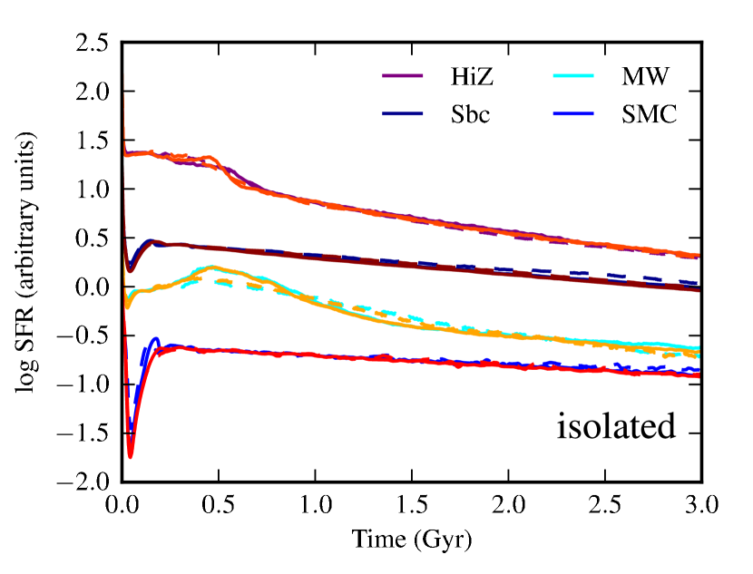
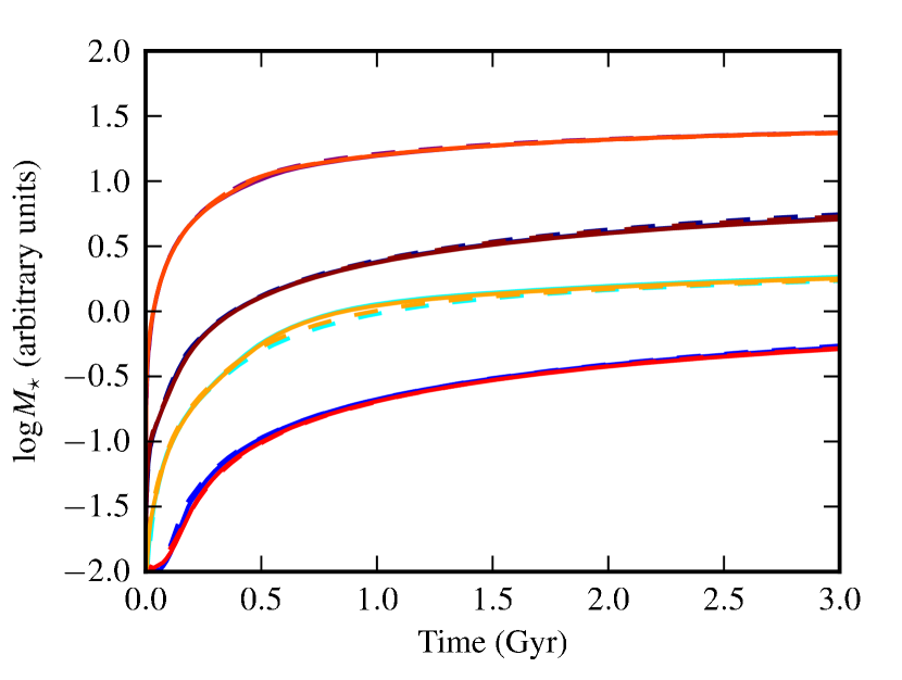
Figure 1: SFR (top) and cumulative stellar mass formed (bottom) versus time (Gyr) for the isolated disc simulations without BHs. The solid and dashed lines denote the higher- and lower-resolution runs, respectively. The blueish colours denote the arepo simulations and the reddish colours denote gadget-3 simulations. For each disc model (from top to bottom, HiZ, Sbc, MW, and SMC), the legend shows the colour used for one of the simulations of that disc. The values for each simulation have been renormalised by an arbitrary constant (kept fixed for all simulations of a given initial disc) so that all runs can be shown clearly on the plot. At $t=3.0$ Gyr, the absolute values of the SFRs for HiZ, Sbc, MW, and SMC are $\sim 4$, $\sim 0.7$, $\sim 0.6$, and $\sim 0.07~{}\mathrm{M_{\odot}{\rm~{}yr}^{-1}}$, respectively. The SFHs are almost identical regardless of the resolution or code used.

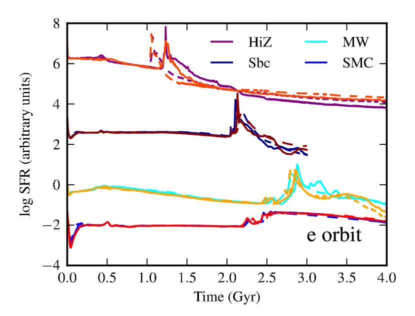
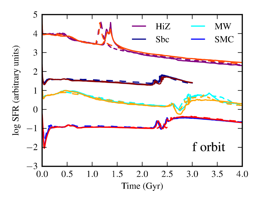
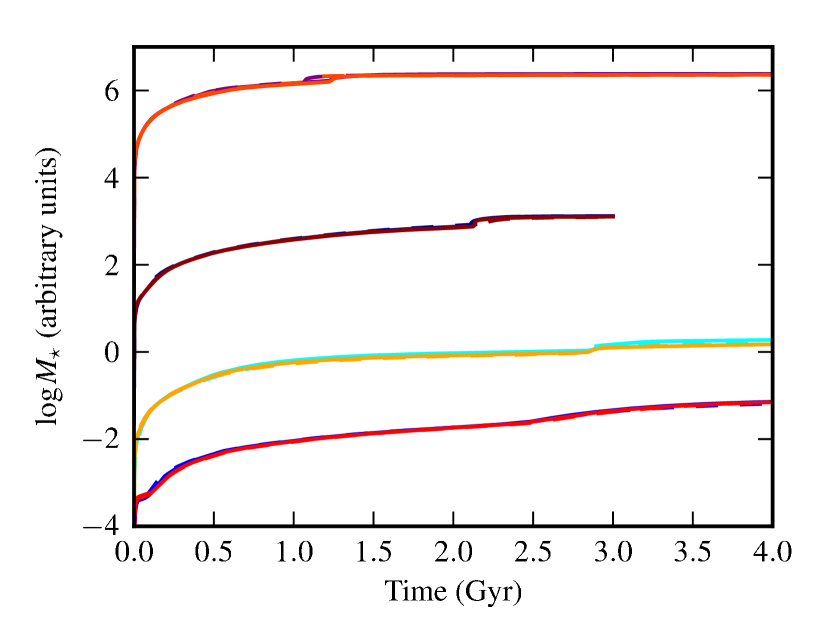
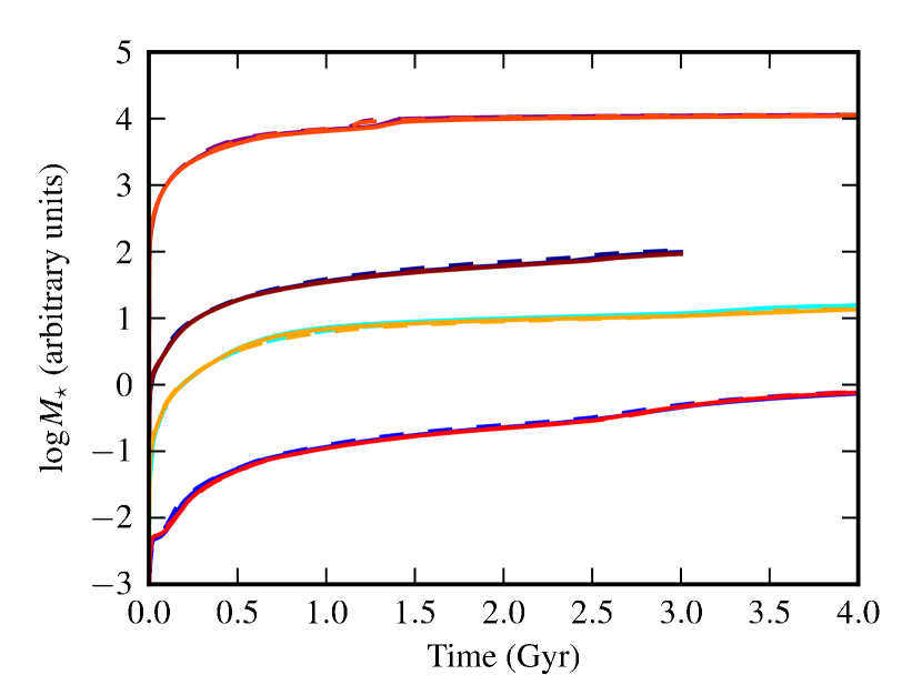
Figure 2: Similar to Fig. 1, but for the e-orbit (left) and f-orbit (right) merger simulations without BH accretion and AGN feedback. At $t=0.5$ Gyr, the SFRs for the HiZ, Sbc, MW, and SMC mergers are $\sim 75$, $\sim 4$, $\sim 10$, and $\sim 0.3~{}\mathrm{M_{\odot}{\rm~{}yr}^{-1}}$, respectively, for both orbits. The SFHs agree less well for these simulations than for the isolated discs. However, the code-dependent differences are minor, and the cumulative stellar mass formed is almost indistinguishable.

A comparison of the star formation histories (SFHs) and cumulative stellar mass formed versus time for the isolated disc simulations is shown in Fig. 1. The solid (dashed) lines indicate the higher (lower) resolution runs, and blueish (reddish) colours indicate arepo (gadget-3) simulations.

The isolated discs (Fig. 1) evolve in the expected manner: after some initial settling into equilibrium, as the gas is consumed (in these idealised simulations, no additional gas is supplied during the simulations), the SFR decreases and the stellar mass formed increases. For the HiZ simulations, there are some minor resolution- and code-dependent differences in the SFHs at $t\sim 0.5$ Gyr. The different Sbc runs are almost identical. The MW simulations exhibit minor resolution-dependent differences in the SFHs throughout the simulation. For the SMC model, there are minor differences in the SFRs of the gadget-3 and arepo simulations at $t\sim 0.2$ Gyr. In all cases, the curves of cumulative stellar mass formed versus time are almost indistinguishable. These results demonstrate that for the isolated disc simulations, the two codes agree very well and the simulations are converged with respect to particle number (at least in terms of their SFHs).

Fig. 2 shows the SFHs for the merger simulations without BH accretion and AGN feedback. As expected from much previous work, the mergers exhibit the following generic evolution. The SFR initially oscillates for a short time as the discs settle into equilibrium. Then, there is a slight elevation when the discs are at first pericentric passage, but the bulges prevent the discs from becoming very unstable. As the discs approach final coalescence, in many cases, strong tidal torques drive gas into the nucleus and fuel a starburst. However, the strength and shape of the starburst depend on the progenitor properties and orbit. After the strong starbursts (HiZ-e, HiZ-f, Sbc-e, and MW-e), the SFR decreases to the pre-merger level or significantly below it. Note that the decrease is driven solely by gas consumption and shock-heating of the gas because these simulations do not include AGN feedback. In the other merger simulations, in which a strong starburst is not induced, the SFR can remain elevated for the duration of the simulation (see especially SMC-e and SMC-f).

As can be inferred from Fig. 2, the agreement for the merger simulations is also excellent, although there are more noticeable differences than for the isolated disc cases. The most prominent difference is that for HiZ-e, HiZ-f, Sbc-e, and MW-e, the time at which the starburst occurs depends on resolution. This is likely caused by resolution-dependent variations in the hydrodynamical drag experienced by the galaxies as they collide, which can slightly alter the merging time-scales. However, for a given resolution, the SFHs during the starburst are similar for the two codes. The most significant, albeit still relatively minor, differences between the arepo and gadget-3 simulations occur after the starbursts, e.g., at $t\ga 2.4$, 2.9, and 2.6 Gyr for Sbc-e, MW-e, and MW-f, respectively. The SFHs do not vary systematically depending on the code used, e.g., for the post-starburst phase of Sbc-e, the arepo SFRs tend to be lower, whereas for MW-e, the opposite is true. As for the isolated discs, the differences in the cumulative stellar mass formed versus time are negligible.

3.1.2 Gas morphologies

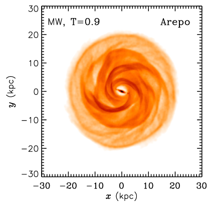
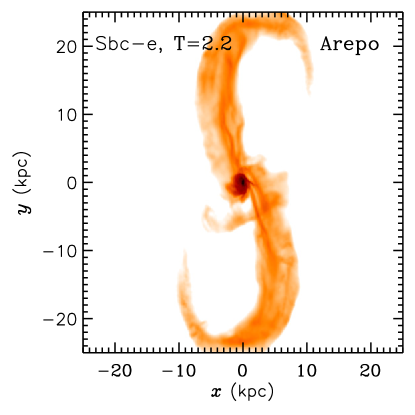
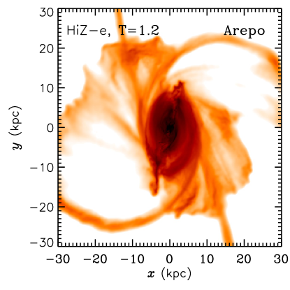
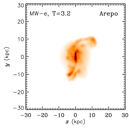
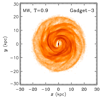
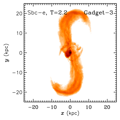
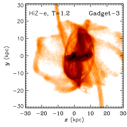
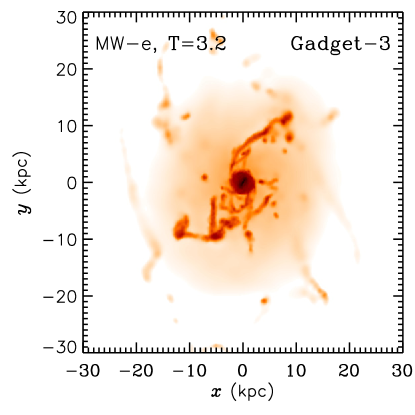
Figure 3: Example gas surface density plots for the following arepo (top) and gadget-3 (bottom) simulations that do not include BH accretion and AGN feedback: isolated MW disc at $t=0.9$ Gyr (first column), Sbc-e merger at $t=2.2$ Gyr (second column), HiZ-e merger at $t=1.2$ Gyr (third column), and MW-e merger at $t=3.2$ Gyr (fourth column). Animations that show the time evolution of the gas surface density for all simulations are available at http://www.cfa.harvard.edu/itc/research/arepomerger/. Typically, the gas morphologies in the gadget-3 and arepo simulations are very similar, but in the post-starburst phase (e.g., column four), the gas morphologies are often clumpier in the gadget-3 simulations and the arepo simulations exhibit less hot halo gas.

The agreement of the SFHs of the gadget-3 and arepo simulations for both the isolated disc and merger simulations indicates that the differences in the numerical schemes do not dramatically affect the global evolution of the simulated systems. However, it is possible that the detailed properties of the simulated mergers differ despite the good agreement for the integrated quantities, and this is indeed the case. Fig. 3 presents gas surface density plots for four different simulation snapshots. (The interested reader is invited to visit the aforementioned URL to view animations that compare the time-evolution of the gas surface density for the highest-resolution runs of all simulations presented in this work.) The top row shows the arepo result, and the bottom row shows the gadget-3 result for the same snapshot and resolution. The first column shows the MW isolated disc at $t=0.9$ Gyr. The arepo and gadget-3 results are qualitatively similar, but the gas distribution appears slightly smoother in the arepo simulation and the orientation of the bar differs. The second column shows the Sbc-e merger at $t=2.2$ Gyr, which is near final coalescence. Again, the morphologies are very similar, but the spatial extent of the tidal tails differs slightly. The third column shows the HiZ-e merger near the peak of the starburst ($t=1.2$ Gyr). Here, the gas distribution is again smoother in the arepo run, and the gas morphology of the nuclear region differs quite dramatically. Finally, the fourth column shows the MW-e merger at $t=3.2$ Gyr ($\sim 0.4$ Gyr after the peak of the starburst). Here, the differences are the most dramatic: the nuclear disc that has re-formed is oriented edge-on in the arepo simulation but face-on in the gadget-3 simulation. This is likely driven by the stochastic nature of the torques acting on the gas that accumulates in the centre of the remnant (e.g., Hernquist & Barnes, 1991). Furthermore, the gadget-3 simulation features a clumpy, extended hot halo that is not present in the arepo simulation.

In general, the arepo morphologies tend to be smoother than those yielded by gadget-3, and the clumps that are often observed in the gadget-3 simulations (and are spurious; e.g., Sijacki et al. 2012) are not present in the arepo simulations. The differences between the two codes are most pronounced during the starburst and post-starburst phases. We discuss the physical reasons for these differences in detail in Section 4.2.

3.1.3 Gas phase structure

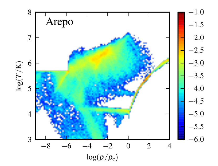
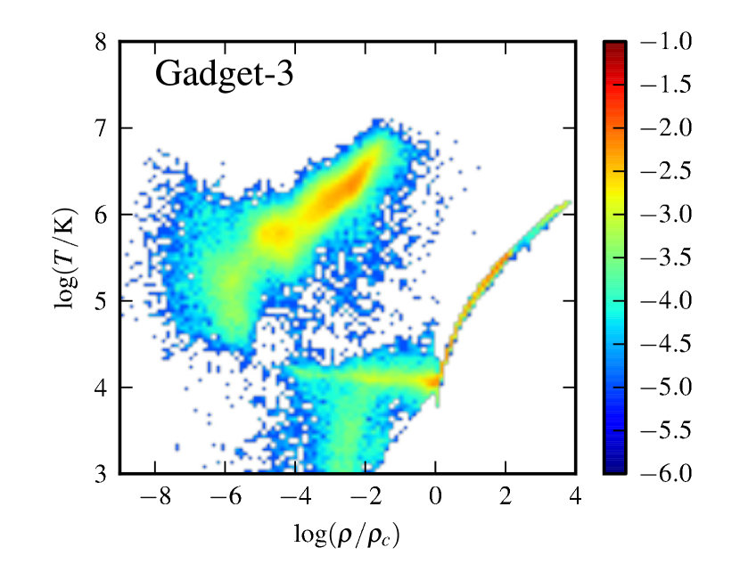
Figure 4: Example phase diagrams (the density is given in terms of the critical density above which gas can be on the Springel & Hernquist 2003 EOS, which corresponds to $n\sim 0.1$ cm^-3) for the MW-e merger simulation without BHs $\sim 400$ Myr after the peak of the starburst ($t=3.2$ Gyr) performed using arepo (left) and gadget-3 (right). (Note that the sharp cutoff in the upper-left corner of the arepo phase diagram is artificial: in arepo, we limit the maximum temperature of the gas below a specified density threshold to avoid wasting computational effort on cells with very low densities and high temperatures, which would have small time steps because of the high sound speed but are unimportant for the hydrodynamics.) Typically, the phase structure of the gas at a fixed time in the arepo and gadget-3 simulations is similar. The largest differences, which are still relatively minor, arise during the starburst and post-starburst periods. During these times, the arepo simulations often contain somewhat less hot gas, as this example demonstrates. The reason is that in arepo, the hot halo gas cools more efficiently, which is why the fourth column of Fig. 3 demonstrates that after the starburst the hot halo is less prominent in the arepo simulations.

We shall now compare the gas phase structure in the gadget-3 and arepo simulations. Animations showing the evolution of the gas phase structure for all simulations are available at the aforementioned URL. For brevity, we will only discuss the general trends and present an illustrative example.

Throughout the simulations, the evolution of the gas phase structure is very similar in the arepo and gadget-3 simulations when BH accretion and AGN feedback are not included. Given the results presented above, this result is not surprising: if the phase structure differed significantly, then the SFHs would not agree so well. As for the gas morphology, the differences are more pronounced in the starburst and post-starburst periods of the simulations. Specifically, the arepo simulations tend to exhibit less low-density, hot halo gas. In both the arepo and gadget-3 simulations, a hot halo forms when gas is shock-heated during final coalescence of the discs. In the arepo simulations, however, the hot halo gas cools more effectively for the reasons discussed in Section 4.2.

Fig. 4 demonstrates this difference. This figure shows example phase diagrams for the post-starburst phase ($t=3.2$ Gyr, $\sim 400$ Myr after the starburst) of the MW-e merger simulation performed using arepo (left) and gadget-3 (right). Note that these correspond to the same simulation and output time as the gas surface density plots shown in the fourth column of Fig. 3. In the arepo simulation, there is less hot halo gas. The enhanced cooling of hot halo gas in the arepo simulation explains why the SFR is somewhat higher in the arepo simulation at this time (see Fig. 2), which is also the case in some of the other merger simulations (e.g., HiZ-e).

3.2 Simulations with BH accretion and AGN feedback

We now compare simulations that include BH accretion and AGN feedback. Here, we use the default accretion and feedback schemes discussed above, but we explore the implications of different choices in Section 3.3.

3.2.1 Star formation histories

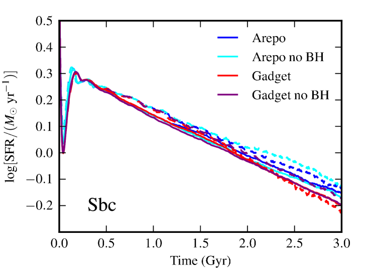
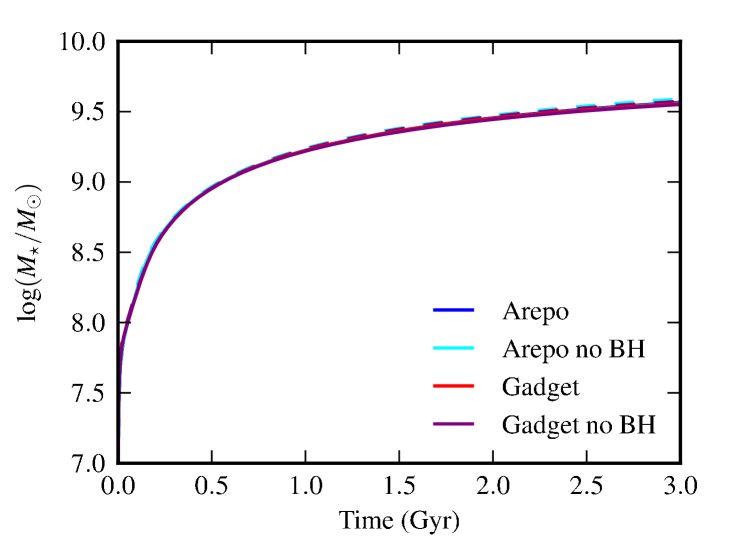
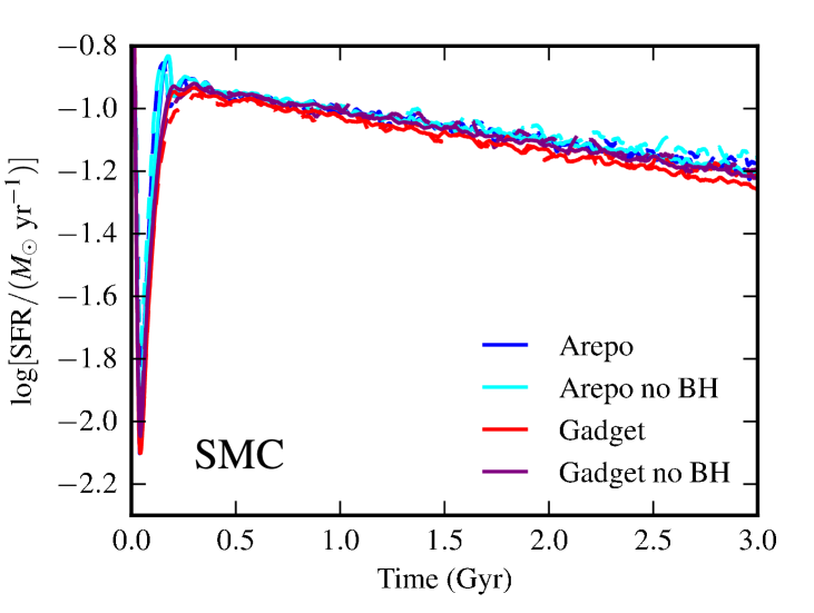
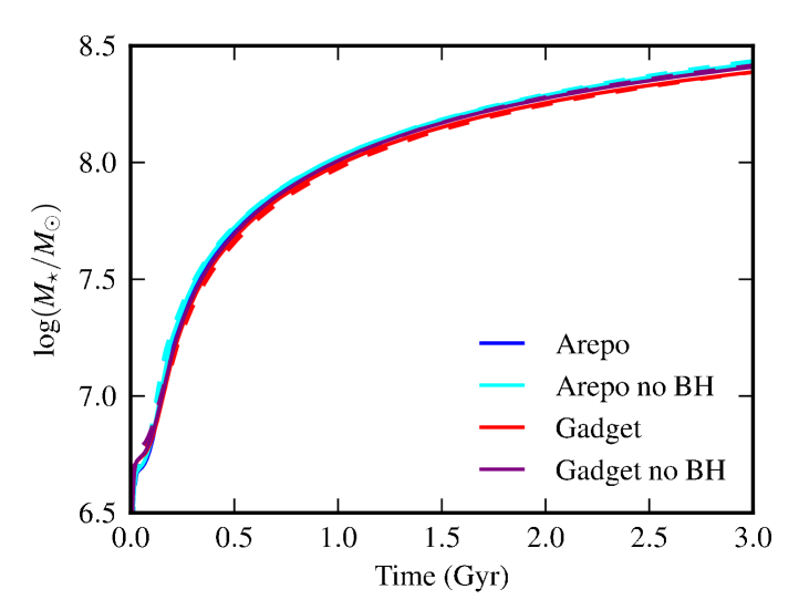
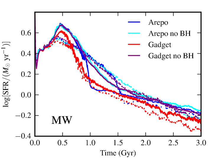
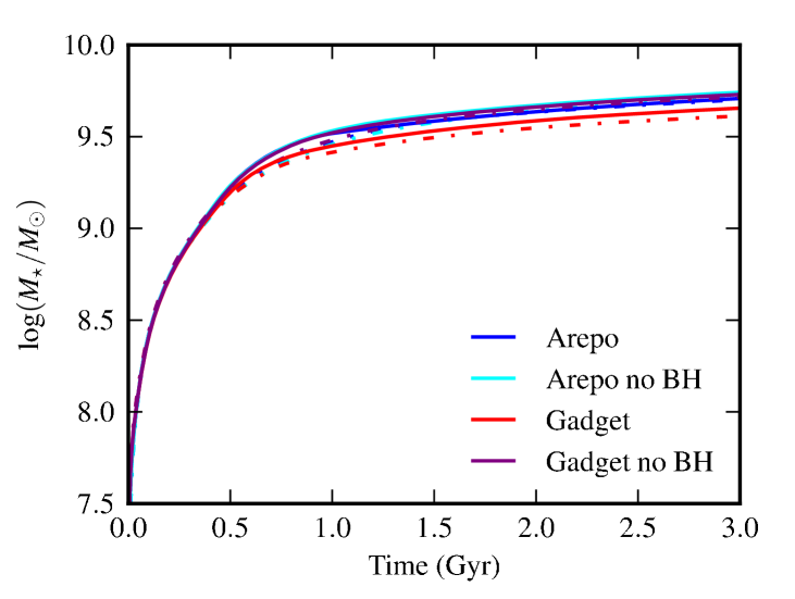
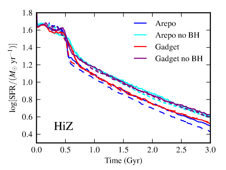
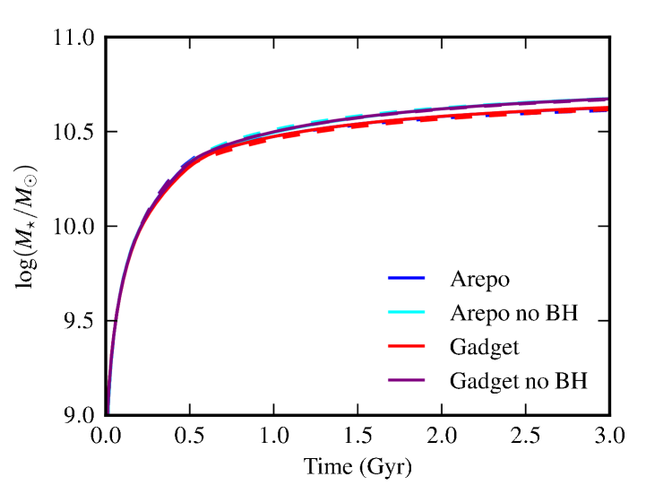
Figure 5: SFHs (left) and cumulative stellar mass formed versus time (right) for the isolated disc galaxy simulations: Sbc (first row), SMC (second row), MW (third row), and HiZ (fourth row). Blue (red) indicates arepo (gadget-3) simulations with BH accretion and AGN feedback; the corresponding simulations without BH accretion and AGN feedback are indicated in cyan (magenta). Solid (dashed) lines indicate higher (lower) resolution simulations. For the MW and HiZ simulations, inclusion of BH accretion and AGN feedback tends to decrease the SFR. When BH accretion and AGN feedback are included, the SFHs agree somewhat less well than when those sub-resolution models are disabled, but the agreement is still quite good.

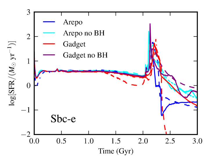
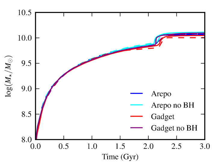
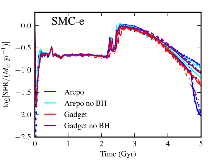
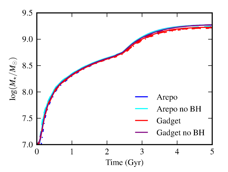
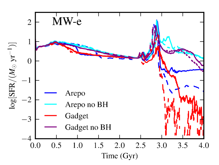
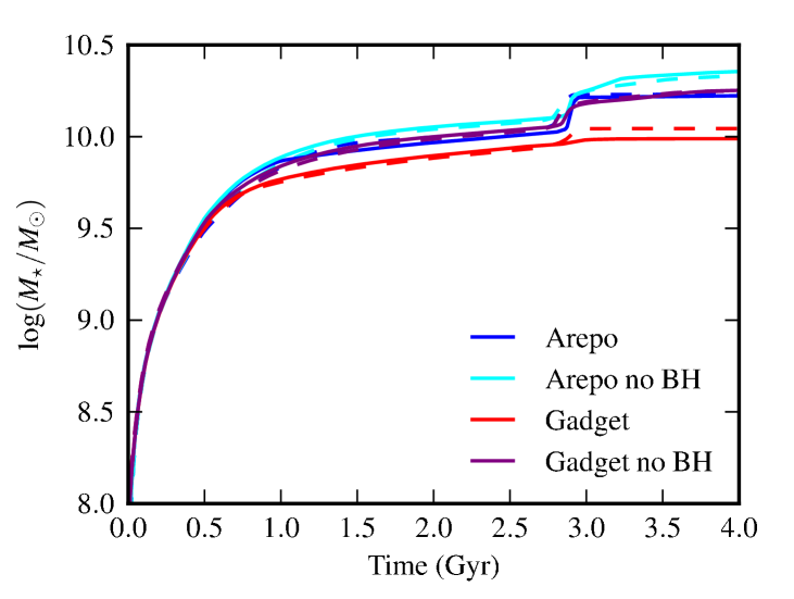
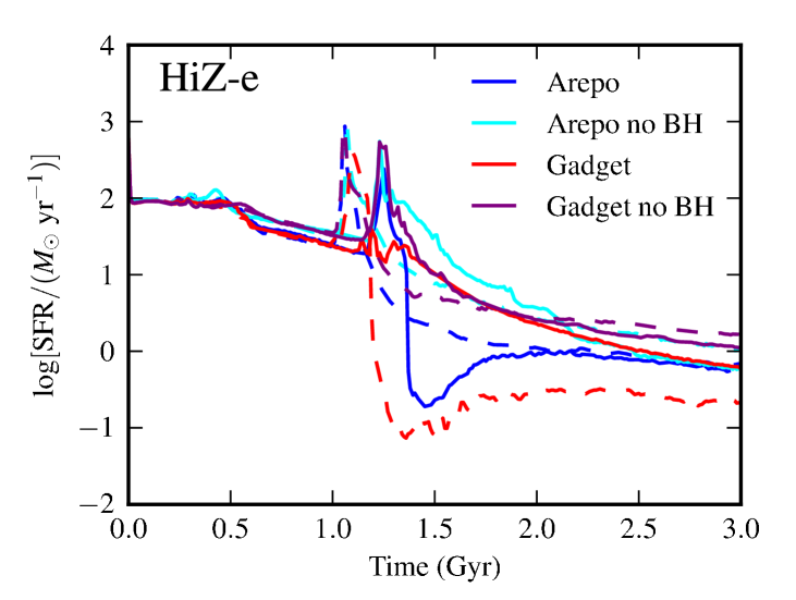
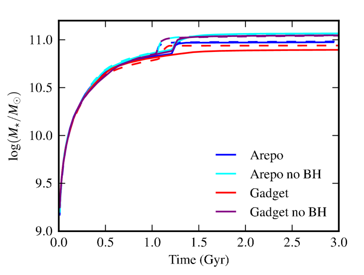
Figure 6: Similar to Fig. 5, but for the e-orbit merger simulations. The SMC-e simulation was performed at a third, higher resolution (R4); the results for this resolution are denoted with dot-dashed lines. The agreement between the arepo and gadget-3 results is less good than for the isolated discs, but the differences are comparable with those between different resolutions. In many cases, AGN feedback decreases the post-starburst SFR, but the strength of the effect depends on both the code used and the resolution.

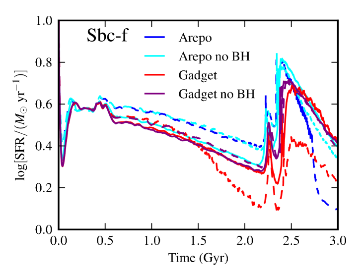
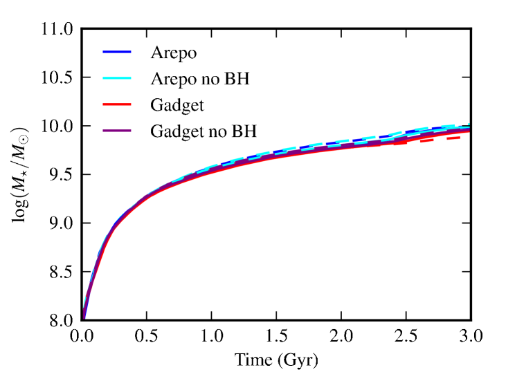
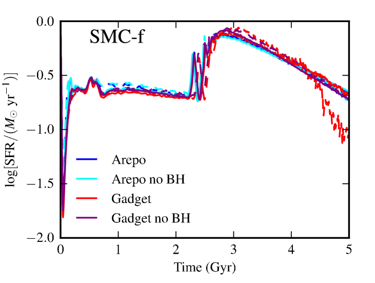
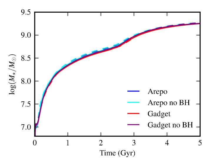
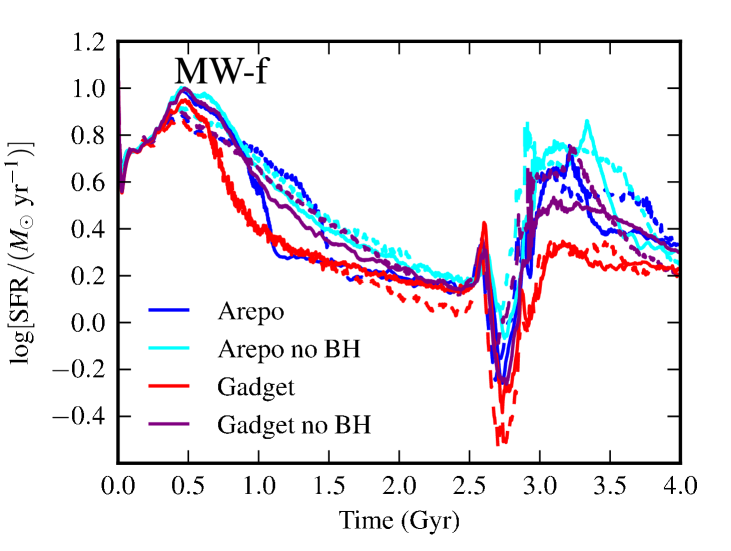
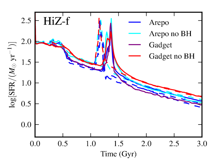
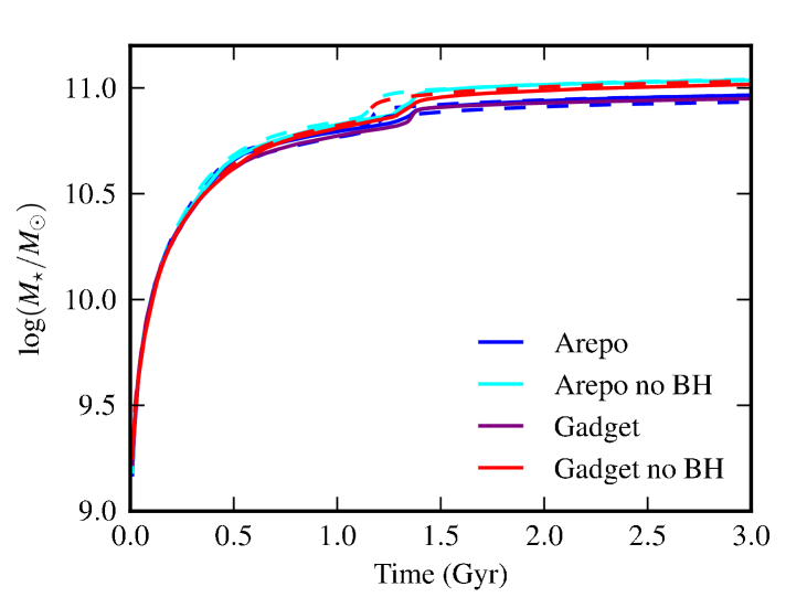
Figure 7: Similar to Fig. 5, but for the f-orbit merger simulations.

Fig. 5 shows the SFHs and cumulative stellar mass formed versus time for the isolated disc simulations. Blue (red) indicates arepo (gadget-3) simulations with BH accretion and AGN feedback; the corresponding simulations without BH accretion and AGN feedback are indicated in cyan (magenta) for comparison. Solid (dashed) lines indicate higher (lower) resolution simulations.

In general, for the isolated disc simulations, the agreement among the SFHs for the two codes and different resolutions is still relatively good, but the differences are clearly more significant than when BH accretion and AGN feedback are disabled. For the Sbc case (first row of Fig. 5), the arepo simulations tend to have slightly higher SFRs, but the differences between the simulations’ SFRs are less than $\sim 0.1$ dex at all times. The cumulative stellar mass formed is indistinguishable. The SFHs for the SMC simulations (second row) agree similarly well, and the cumulative stellar mass formed is nearly the same. For the MW simulations (third row), the SFRs differ by as much as $\sim 0.3$ dex, but the resolution-dependent variations are as significant as those between the codes and the differences for simulations that vary only in whether they include BH accretion and AGN feedback. In this case, the total stellar mass formed over the course of the simulations (3 Gyr) is $\sim 0.1$ dex less in the gadget-3 simulations with AGN feedback, but all other simulations agree very well. Finally, the SFRs of the HiZ isolated disc simulations (fourth row) can vary by as much as $\sim 0.2$ dex, and the primary cause of the difference is whether BH accretion and AGN feedback are included (in such simulations, the SFRs are systematically lower, as expected). However, the stellar mass formed is the same to within $\la 0.1$ dex.

Figs. 6 and 7 show the SFHs and cumulative stellar mass formed versus time for the e-orbit and f-orbit merger simulations, respectively. For brevity, we will not discuss each panel individually but rather highlight general trends. For a given progenitor combination and orbit, the shapes of the SFHs are qualitatively similar for both codes and all resolutions (except in the cases for which AGN feedback significantly impacts the post-starburst SFR). However, there are significant quantitative code- and resolution-dependent differences. For many of the simulations (i.e., Sbc-e, SMC-e, HiZ-e, SMC-f, and HiZ-f), the SFHs are almost identical up to final coalescence. If a strong starburst is triggered, the precise time and amplitude of the starburst can vary depending on the code and resolution. In some – but not all – cases (Sbc-e and MW-e, in particular), inclusion of AGN feedback causes the post-starburst SFR to decrease more rapidly compared with the corresponding simulations without AGN feedback. Although the SFHs differ significantly at some times, the cumulative stellar mass formed versus time is often very similar for the different codes and resolutions, as we saw above for the simulations without AGN feedback and the isolated disc simulations with AGN feedback. In most cases, the cumulative stellar mass formed differs by less than $\sim 0.1$ dex at all times. The MW-e merger simulations exhibit the most significant differences in the cumulative stellar mass formed: when AGN feedback is included, the cumulative stellar mass formed in the arepo simulations is $\sim 0.25$ dex greater than in the gadget-3 simulations.

3.2.2 BH masses

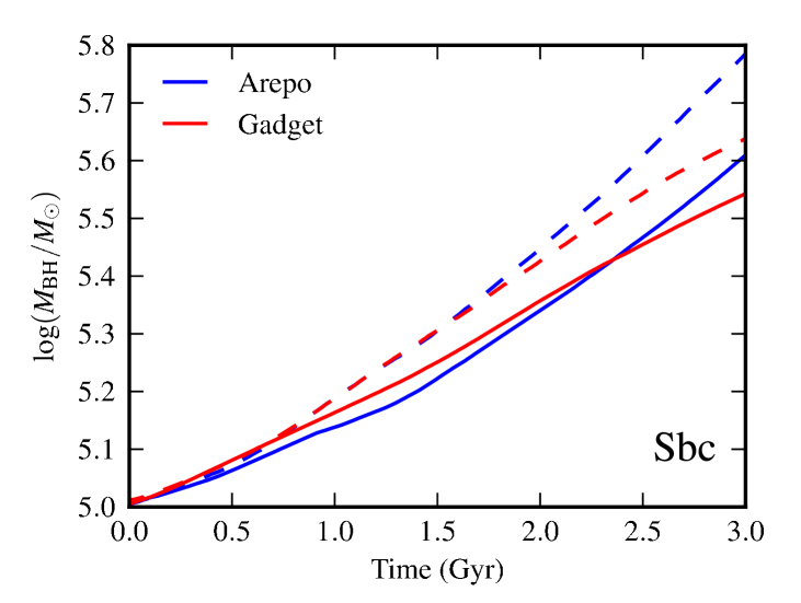
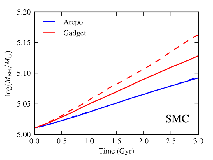
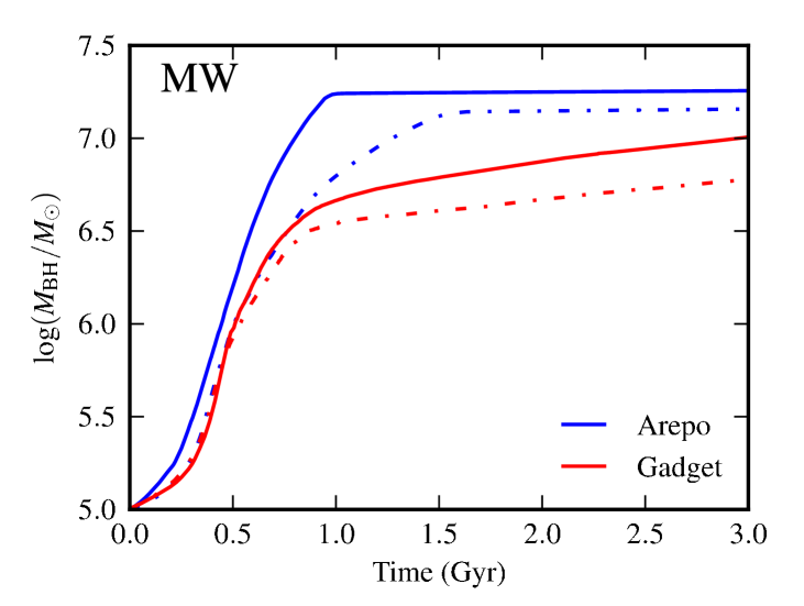
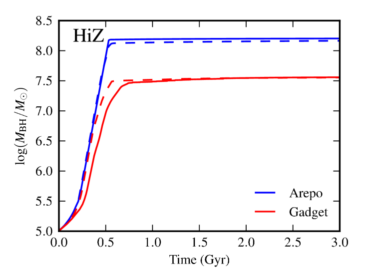
Figure 8: BH mass versus time for the isolated disc galaxy simulations: Sbc (top left), SMC (top right), MW (bottom left), and HiZ (bottom right). Blue (red) indicates arepo (gadget-3) simulations with BH accretion and AGN feedback. Solid (dashed) lines indicate higher- (lower-) resolution simulations. For these simulations, the BH masses are reasonably well converged with respect to particle number, and the code-dependent effects are more significant than the differences between the two resolutions. For all but the SMC simulation, for a given particle number, arepo yields more massive BHs.

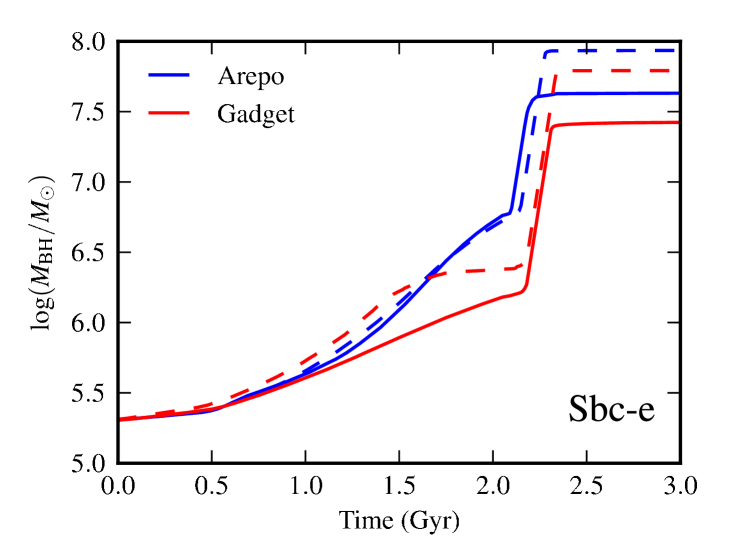
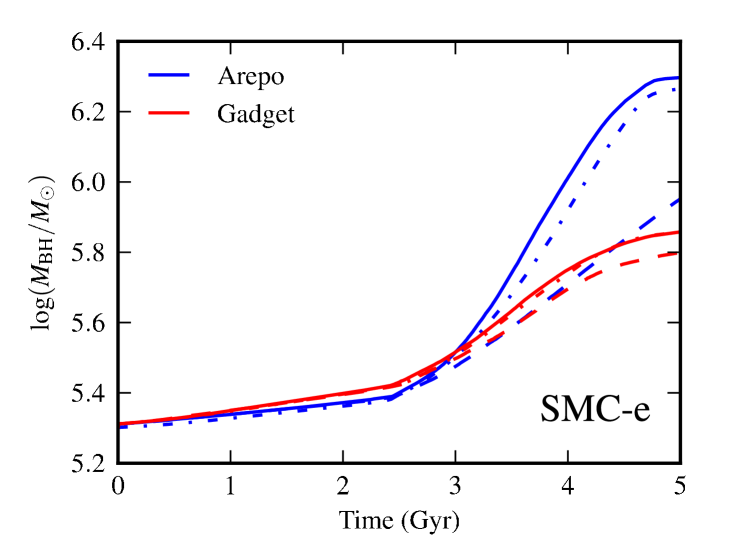
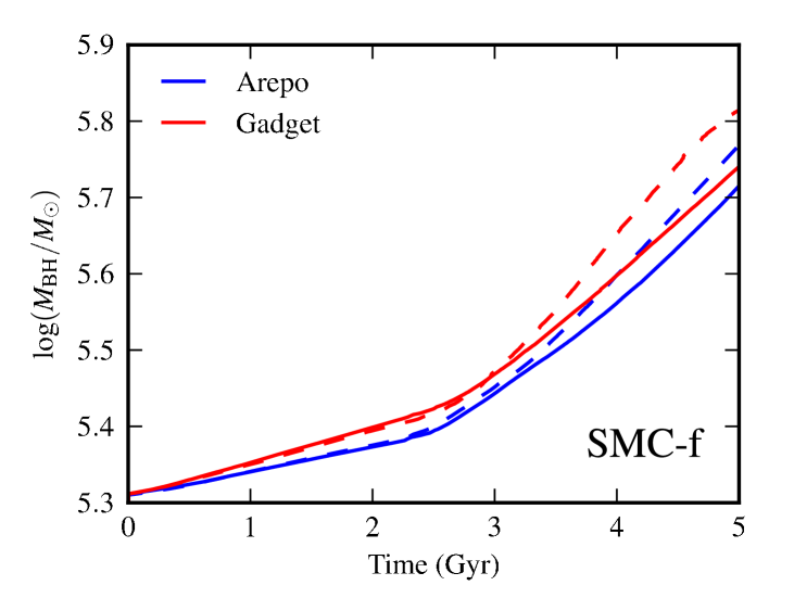
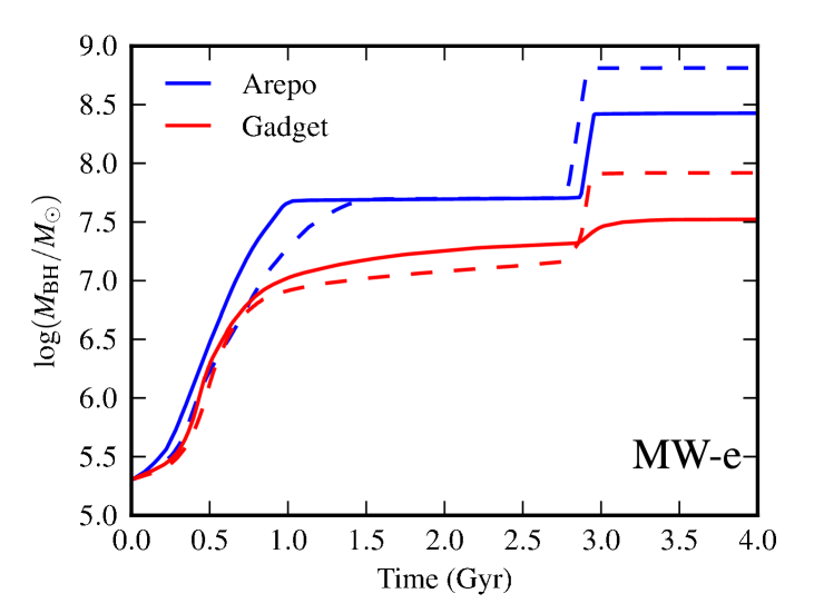
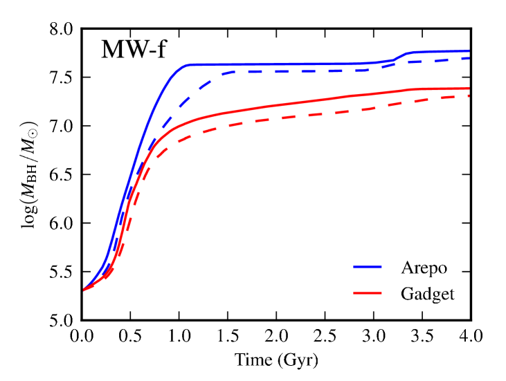
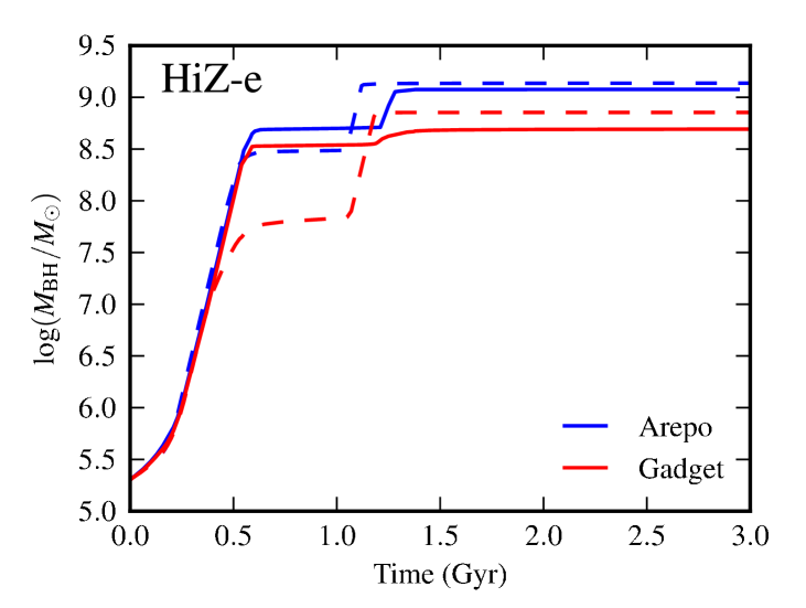
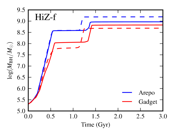
Figure 9: Similar to Fig. 8, but for the merger simulations: Sbc (first row), SMC (second), MW (third), and HiZ (fourth). The left (right) column shows the results for the e-orbit (f-orbit) merger simulations. Note that the SMC-e merger was run at a third, higher resolution (R4); the results are denoted with dot-dashed lines. During the mergers, the BH masses can increase by multiple orders of magnitude. The code- and resolution-dependent differences in the BH masses can be as large as a factor of a few. The differences with resolution are not systematic. For all but the SMC-f simulations, for a given resolution, the BH masses yielded by arepo are greater than those yielded by gadget-3.

Another quantity of interest is the BH mass versus time because differences in the BH masses would alter the strength of the AGN feedback and thereby influence whether or not the merger remnants lie on the $M_{\rm BH}-\sigma$ relation (Ferrarese & Merritt, 2000; Gebhardt et al., 2000). It is natural to expect that the BH mass evolution is more code- and resolution-dependent than the SFH because the BH growth depends sensitively on the gas conditions in the nuclear region(s) and could thus be affected by small-scale variations that would not significantly alter the integrated SFH.

Fig. 8 shows the BH mass versus time for the isolated disc simulations. In the Sbc and SMC simulations, the BHs grow by only a modest amount ($\la 0.8$ and $\la 0.15$ dex, respectively) over the 3.0 Gyr of the simulations. In the MW and HiZ simulations, the BHs rapidly increase in mass by 2-3 orders of magnitude. This strong BH growth in the absence of a merger is driven by bar instabilities, which is clear from examination of the gas morphologies. The BH growth terminates once the gas near the BH is consumed or expelled.

For a given code, the final BH masses in the isolated disc simulations differ with resolution by $\la 0.2$ dex. However, the code-dependent variations can be more significant. In particular, note that the final BH masses in the arepo HiZ simulations are a factor of $\sim 5$ greater than those in the gadget-3 simulations.

The BH mass evolution for the merger simulations is shown in Fig. 9. In these plots, the total mass of all BHs – recall that each progenitor disc is seeded with a BH – is plotted. For a given progenitor, the BHs grow significantly more in the merger simulations than in the isolated disc simulations. The SMC-f merger exhibits the weakest growth ($\sim 0.5$ dex), and the HiZ merger simulations exhibit the strongest BH growth (almost four orders of magnitude). As for the SFHs, the code- and resolution-dependent differences amongst the BH masses in the merger simulations are more significant than for the isolated disc simulations. In many – but not all – examples, the BH masses are greater in the arepo simulations than in the gadget-3 runs. The resolution-dependent variations (which are at most $\sim 0.6$ dex and usually significantly less) are typically less than the code-dependent differences (for a given resolution, these can be as great as an order of magnitude), and the resolution dependence is not systematic. Consequently, for a given code, the final BH masses should be considered uncertain by as much as a factor of a few. This reflects the high degree of non-linearity in the feedback-regulated BH growth. Any small variation in the local gas conditions at the BH’s position can influence its exponential growth rate and hence become strongly amplified with time. Note also that the BH accretion histories can differ significantly depending on the resolution and code; thus, during the merger, the BH masses at a given time can differ more significantly than the final BH masses (i.e., the BH masses after the BH growth has terminated, which can occur at different times for different resolutions and codes).

Interestingly, for the SMC-e merger, which was simulated at three resolutions, the BH mass evolution in the two higher-resolution (resolutions R3 and R4) simulations performed with a given code is almost identical, but the $\sim 0.4$ dex difference in the final BH masses yielded by the two different codes persists. Thus, it is possible that the BH masses yielded by a given code would converge if all simulations were performed at even higher resolution, but we have not performed such simulations because of the computational expense and because the code-dependent differences, which are the focus of this work, remain even for the highest-resolution SMC-e simulations.

3.2.3 Gas morphologies

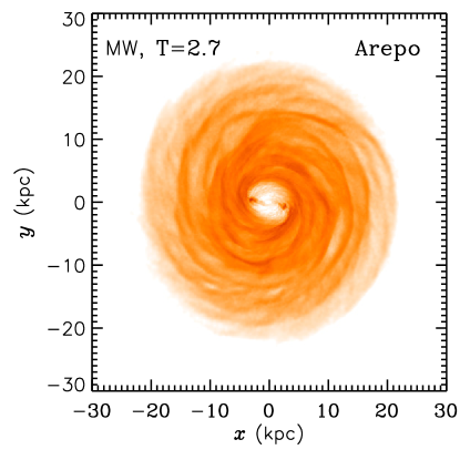
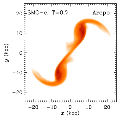
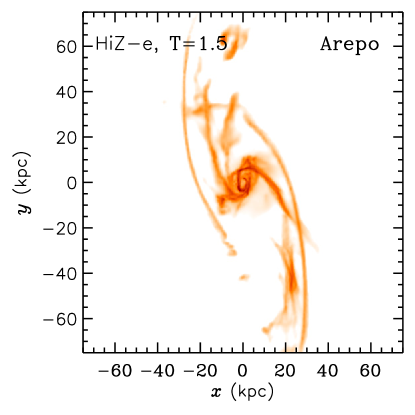
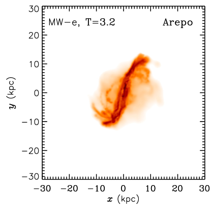
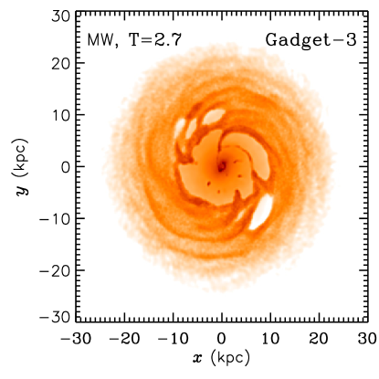
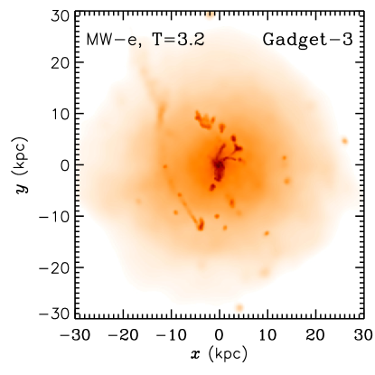
Figure 10: Example gas surface density plots for the following arepo (top) and gadget-3 (bottom) simulations that include BH accretion and AGN feedback: isolated MW disc at $t=2.7$ Gyr (first column), SMC-e merger at $t=0.7$ Gyr (second column), HiZ-e merger at $t=1.4$ Gyr (third column), and MW-e merger at $t=3.2$ Gyr (fourth column). As for the simulations without BH accretion and AGN feedback, in the starburst and post-starburst phases, the gadget-3 results feature more prominent hot haloes and spurious clumps.

Fig. 10 shows example gas surface density plots for the arepo (top row) and gadget-3 (bottom row) simulations with BH accretion and AGN feedback. As for the simulations without BH accretion and AGN feedback, the morphologies are qualitatively similar, but the details differ. Furthermore, as for the SFHs, the code-dependent differences in the gas morphologies are more significant when BH accretion and AGN feedback are included. The first column shows the MW isolated disc at $t=2.7$ Gyr. At this time, a bar is evident in the arepo simulation and much of the gas in the central region has been consumed because of the bar instability. In the gadget-3 simulation, a bar is not evident; rather, a large, irregularly shaped cavity, which contains some small clumps of dense gas, has formed. Part of the reason for the significant differences between the arepo and gadget-3 results is that in the arepo simulations, the BH can only consume gas that is within 50 pc, whereas in gadget-3, the region from which gas is accreted grows as the gas near the BH is depleted because a fixed number of neighbours is used to calculate the SPH density estimate. Note, however, that generically, holes tends to form around the BHs for the following physical reason: in the quiescent state that is eventually reached in isolation or at the end of a merger (when the BH growth has effectively shut off), a small bubble of hot, low-density gas around the BH is created by the pressure that is sustained in our feedback model by the residual accretion.

The second column shows the SMC-e merger simulation at $t=0.7$ Gyr (after first pericentric passage). The results of both codes exhibit extended, smooth tidal features, and the morphologies are almost indistinguishable. This column exemplifies the good agreement that is characteristic of the pre-starburst phase of the merger simulations.

The third column of Fig. 10 shows the HiZ-e merger near the peak of the starburst ($t=1.4$ Gyr). Some of the filamentary structure is similar in the arepo and gadget-3 simulations, but the detailed morphologies differ significantly. As noted above, the gadget-3 result exhibits many spurious clumps of gas that are not present in the arepo simulation.

Finally, the fourth column shows the MW-e merger at $t=3.2$ Gyr, $\sim 400$ Myr after the starburst. Note that for comparison, this is the same simulation and time as shown in the fourth column of Fig. 3, except that BH accretion and AGN feedback are included here. For a given code, the gas morphologies are similar to those of the simulations for which BH accretion and AGN feedback were not included (Fig. 3). One notable difference is that in the gadget-3 simulation, the gas disc is less pronounced and the hot halo is more prominent. Once again, the gadget-3 simulation features an extended halo of hot gas and spurious clumps, both of which are not present in the arepo simulation. Note that in this example, the code-dependent differences in the gas morphologies are more significant than those caused by the inclusion of AGN feedback. This result is a counterexample to the conclusion of Scannapieco et al. (2012) regarding the effects of various star formation and stellar feedback models compared with differences between codes and implies that it is highly desirable to use the most accurate hydrodynamical solver possible.

3.2.4 Gas phase structure

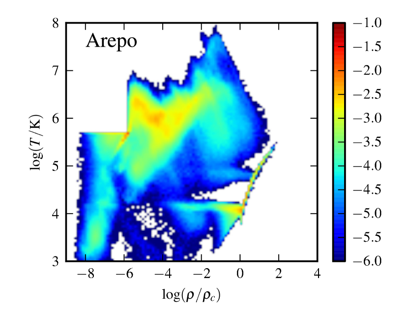
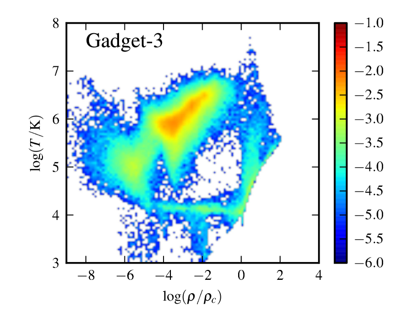
Figure 11: Similar to Fig. 4, but for the MW-e simulations with BH accretion and AGN feedback at the same time as in Fig. 4 ($t=3.2$ Gyr, $\sim 400$ Myr after the peak of the starburst and AGN activity). For both codes, AGN feedback results in more hot halo gas. As for the simulations without AGN feedback, the gadget-3 simulation features hot halo gas than the arepo simulation; in the latter, the hot halo gas cools more efficiently on to the EOS.

As for the simulations without BH accretion and AGN feedback, the gas phase structure in the gadget-3 and arepo simulations is similar in the pre-starburst phase but can differ significantly during and after the starburst. Again, we only present one example to illustrate the characteristic differences here, but the interested reader can visit the aforementioned URL to examine the evolution of the gas phase structure for all simulations.

Fig. 11 shows gas phase diagrams for the MW-e simulations with BH accretion and AGN feedback at the same time as in Fig. 4 ($t=3.2$ Gyr, $\sim 400$ Myr after the peak of the starburst and AGN activity). For a given code, the inclusion of AGN feedback causes there to be more gas in the hot halo and correspondingly less gas on the EOS (the thin line in the lower-right corner). As for the simulations that did not include AGN feedback, the gadget-3 simulation features more hot halo gas than the arepo simulation, in which the hot halo gas cools more efficiently.

3.3 Tests of the BH accretion and AGN feedback models

Here, we present various tests that demonstrate the effects of the different treatments of BH accretion and AGN feedback discussed above. We use the SMC analogue as one test case. Whereas for this simulation, the differences in the results are small in an absolute sense, they are systematic and can have more significant effects in other simulations. We chose to use the SMC analogue as a test case because the SFH and BH growth are comparatively simple; thus, differences can be more easily understood. Furthermore, the BH grows very little ($M_{\mathrm{BH}}\sim 10^{5}~{}\mathrm{M_{\odot}}$, the seed mass, throughout the simulation) and should have a negligible effect on the SFH of the galaxy. Thus, the ‘no BH’ case can be used as the baseline with which to compare the other runs; ideally, the SFHs should be the same for the BH and ‘no BH’ cases. We also investigate the effects of different BH accretion and AGN feedback for the MW-e merger simulation. In this significantly more complicated case, the interpretation of the comparisons among the different treatments of BH accretion and AGN feedback is less straightforward, but many of the effects observed for the SMC case are also observed here. The tests presented here justify our fiducial choices for the BH accretion and feedback implementations and demonstrate some important numerical effects that are not always appreciated in the literature.

3.3.1 Refinement near the BH

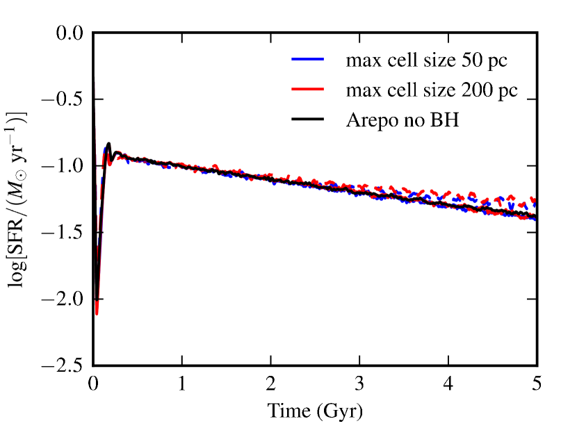
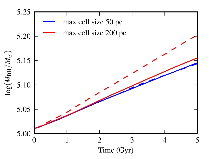
Figure 12: Demonstration of the effect of limiting the cell size near the BH for the isolated SMC disc simulation. The top (bottom) panel shows the SFH (BH mass versus time). The blue (red) lines show the results when cells that are less than 500 pc from the BH are forced to have size less than 50 (200) pc. The higher-resolution simulation with BH accretion and AGN feedback disabled is shown in black. When the maximum cell size near the BH is 50 pc, the agreement between the two resolutions is excellent.

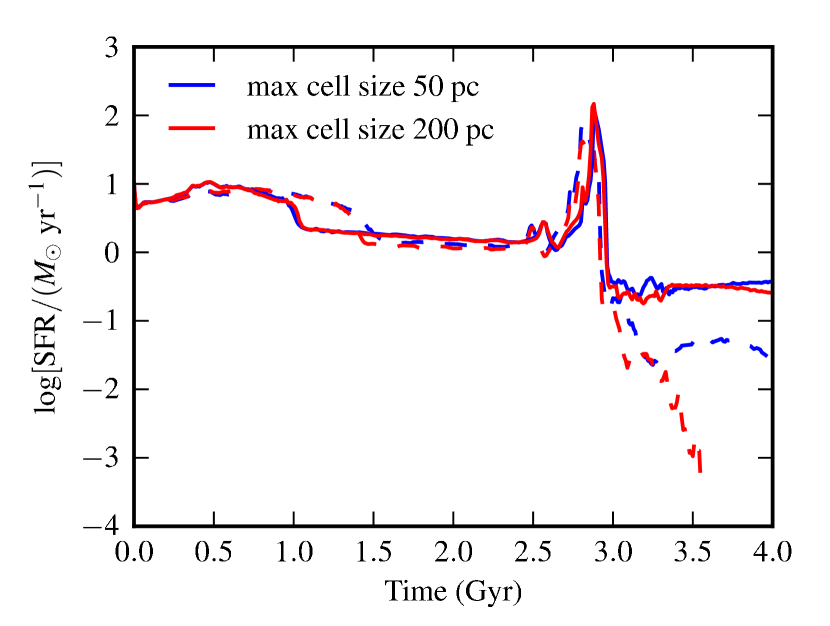
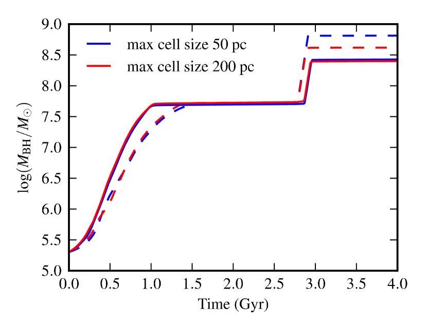
Figure 13: Similar to Fig. 12, but for the MW-e merger. The results are almost independent of the $r_{\rm max}$ value for the higher resolution because the resolution around the BH is sufficiently high without the forced refinement. The final BH masses for the two resolutions agree better when $r_{\rm max}=200$ pc, but this agreement does not indicate better convergence. See the text for details.

In SPH, as the gas density in the immediate vicinity of a BH decreases because of gas consumption and expulsion, the radius over which the density is calculated increases because the number of neighbours used for the density estimate and the particle masses are fixed. Thus, in some situations, the BH accretion rate can be overestimated and gas fuels the BH from unphysically large scales; this is especially problematic in cosmological simulations, for which the resolution is often not better than a kiloparsec. In arepo, the standard cell refinement scheme attempts to keep cell masses comparable; thus, a similar effect, in which cells near the BH grow large, can occur. However, unlike in SPH, we can overcome this potential problem by preventing cells near the BH from becoming too large and using the gas density of the cell that contains the BH to calculate the accretion rate. Consequently, if the gas density in the vicinity of the BH decreases, the accretion rate decreases concomitantly.

Fig. 12 demonstrates the effects of limiting the maximum cell size near the BH particle for the SMC isolated disc case. We force cells located within 500 pc of the BH to be refined if their size is greater than some value $r_{\rm max}$. We show the results for $r_{\rm max}=50$ and 200 pc in Fig. 12. The top panel indicates that the choice of $r_{\rm max}$ has no effect on the SFH, and the slight difference between the different resolutions at late times is independent of $r_{\rm max}$.

However, the growth of the BH differs systematically. For both resolutions, the BH grows more when $r_{\rm max}=200$ pc because of the effect described above, and the consequences are more severe for the lower-resolution simulation. When $r_{\rm max}=50$ pc, the final BH mass is slightly less and the two different resolutions agree perfectly.

Fig. 13 shows the results of changing $r_{\rm max}$ for the MW-e merger simulation. In this case, the SFH is better converged when a maximum cell when $r_{\rm max}=50$ pc. For the higher-resolution simulations, the BH growth history is unaffected by the choice of $r_{\rm max}$. Thus, for this resolution ($\epsilon_{\mathrm{bar}}=60$ pc), the refinement near the BH is sufficiently high even without forcing refinement. Interestingly, the final BH mass of the lower-resolution simulation with $r_{\rm max}=200$ pc agrees better with that of the higher-resolution simulations than when $r_{\rm max}=50$ pc. In this case, allowing larger cells near the BH by setting $r_{\rm max}=200$ pc serves to mitigate some of the resolution dependence: in the lower-resolution simulation with $r_{\rm max}=50$ pc, during the starburst at final coalescence, the central gas density is greater than in the higher-resolution runs. Consequently, the BH grows more rapidly during that time. Using $r_{\rm max}=200$ pc results in a decreased central gas density and thus less-massive BH. However, this result should not be taken as an indication that the BH mass is better-converged when $r_{\rm max}=200$ pc: if the BH mass were truly converged, the $r_{\rm max}=50$ pc simulation should agree at least as well because in this simulation, the number of resolution elements is greater than or equal to that of the lower-resolution simulation.

3.3.2 BH accretion rate calculation

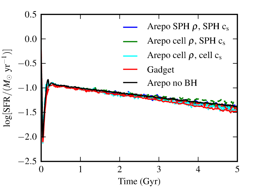
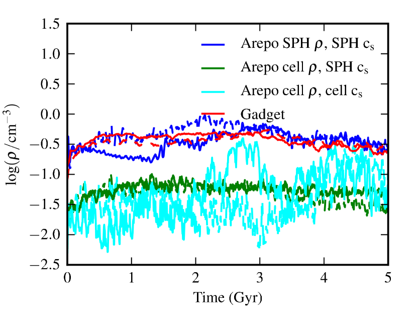
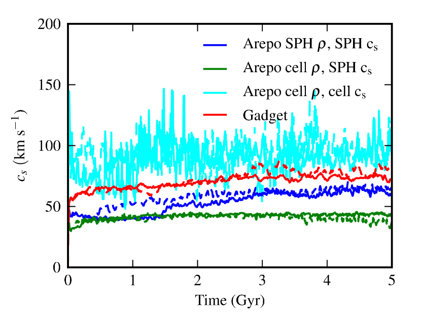
Figure 14: Comparison of different methods for calculating the BH accretion rate in arepo. Either the cell value or the SPH density estimate of both the gas density and sound speed near the BH can be used. Different combinations are shown (see the legend). For comparison, the arepo simulation with no BH and the gadget-3 simulation with BH accretion and AGN feedback are also shown. Solid (dashed) lines indicate higher- (lower-) resolution simulations. The panels show the following quantities versus time: the SFR (upper left), the BH mass (upper right), and the gas density (lower left) and sound speed (lower right) estimates used to calculate the accretion rate (the last two quantities have been smoothed with a median filter of size 1001 time steps for plotting purposes). Use of the cell density and SPH estimate for the sound speed yields the best convergence, and the convergence is also good when the cell sound speed is used. Still, we have opted to use the SPH estimate for the sound speed in our fiducial model because unlike the cell density, the cell sound speed is very noisy.

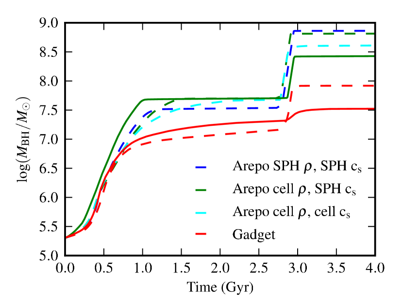
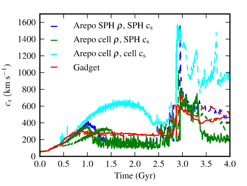
Figure 15: Similar to Fig. 14, but for the MW-e merger. As for the SMC isolated disc, use of the cell sound speed to calculate the BH accretion rate results in a smaller final BH mass because the cell sound speed can be more than a factor of three greater than the SPH estimate.

To calculate the BH accretion rate using equation (1), we require the gas density and sound speed near the BH. In arepo, both quantities can be estimated in a manner analogous to that in SPH, i.e., by averaging over some number of nearest neighbour cells (typically, 32). However, it is also possible to use the gas density and sound speed for the cell in which the BH is located. In principle, the cell values should be more representative of the conditions near the BH and thus ensure a more physical calculation of the accretion rate, but they may be too noisy to be useful. We will explore the effects of these choices now.

Fig. 14 demonstrates the variations that arise from using different methods to calculate the BH accretion rate in arepo for the SMC isolated disc case. The gadget-3 results are shown for comparison. In all cases, the mass over which the feedback energy is distributed is kept constant, i.e., the number of cells or particles over which the energy is distributed is increased as the cell mass is decreased. Furthermore, cells within 500 pc of the BH are forced to have size less than $r_{\rm max}=50$ pc.

The differences in the SFH (upper-left panel) for the various treatments are small and comparable with the resolution-dependent differences. The BH growth history, in contrast, can be affected significantly; the upper-right panel indicates that the final BH mass can differ by as much as 0.4 dex, and the effect in merger simulations can be even larger. The BH grows most in arepo when the SPH density and sound speed are used (the blue curve). The reason is that, as shown in the lower-left panel, in arepo, the SPH density estimate is systematically greater than the cell density (and similar to the gadget-3 density). The gadget-3 simulations (red curve) exhibit the next highest BH growth; the reason that they feature less growth compared with the analogous arepo simulations is that the SPH sound speed estimate (lower-right panel) is systematically higher in gadget-3 than arepo.

When the cell density is used, the BH grows less because the cell density is systematically lower than the SPH density. The growth is most suppressed when the cell sound speed is used (cyan curve) because the cell sound speed is systematically higher than the SPH sound speed. Furthermore, the cell sound speed is very noisy, with variations of $\ga 50$ km$\rm s^{-1}$ from the mean value, and the cell density is significantly more noisy when the cell sound speed is used to calculate the BH accretion rate (compare the cyan and green curves in the lower-left panel of Fig. 14).

Fig. 15 compares the different BH accretion rate treatments for the MW-e merger simulation. As for the SMC isolated disc case, the BH grows most when the SPH estimates for the gas density and sound speed are used to calculate the accretion rate. Using the cell density rather than the SPH estimate results in a very similar final BH mass. Furthermore, using both the cell density and sound speed results in the smallest final BH mass of the three lower-resolution simulations because the cell sound speed can be more than a factor of three greater than the SPH estimate. Although the differences in the BH masses caused by varying the sub-resolution model accretion rate calculation are significant ($\sim 0.3$ dex), they are less than the differences between the two resolutions for a fixed code and those between the two codes for a fixed number of particles/cells.

Based on these results, we chose to use the cell density for our production runs because this is more representative of the density near the BH than is the SPH density, yet the two have comparable amounts of noise. However, we chose to use the SPH estimate for the sound speed because the cell value is too noisy.

3.3.3 AGN feedback

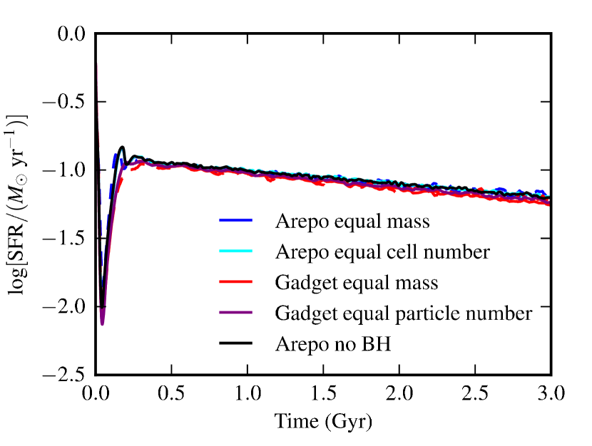
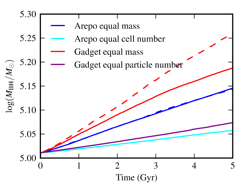
Figure 16: Similar to Fig. 14, but for different methods of distributing the BH feedback energy. In both gadget-3 and arepo, keeping the mass – rather than the number of particles or cells – over which the AGN feedback energy is distributed fixed with resolution yields the best convergence. Thus, we have used this as our standard method. Note that the convergence of the BH masses in the arepo simulations is excellent when this treatment is used.

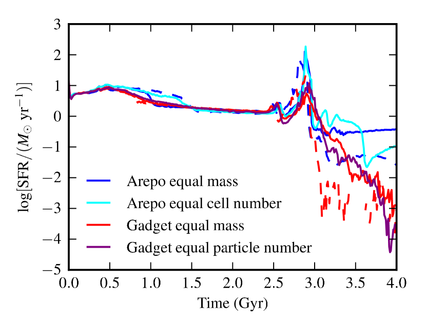
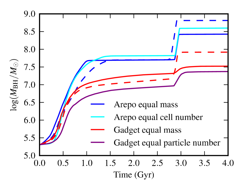
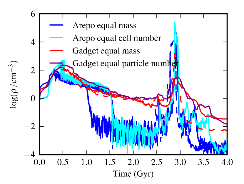
Figure 17: Similar to Fig. 16, but for the MW-e merger. In this case, keeping the mass over which the feedback energy is distributed constant yields a better-converged final BH mass for gadget-3 but not arepo.

The manner in which the AGN feedback energy is distributed can also affect the BH growth. As explained in Section 2.3.2, our preferred method is to keep the mass over which the feedback energy is distributed (the ‘feedback mass’) constant. Thus, for higher-resolution runs, in which the particle/cell mass is lower, the number of particles/cells over which the feedback energy is distributed should be increased. However, this is not the only possible approach; an alternative approach is to keep the number of particles/cells over which the feedback energy is distributed fixed. But, as we will show now, this causes a stronger resolution dependence, which is undesirable for a sub-resolution model.

Fig. 16 demonstrates the differences between these two choices for the SMC isolated disc case. As in the previous test, there are minor variations in the SFHs at late times, but the magnitude of the difference is similar to that caused by varying the resolution. However, varying the method for distributing the feedback energy causes significant and systematic changes in the BH growth history. First, note that the dashed and solid blue lines, which correspond to the lower-resolution arepo simulation and the higher-resolution simulation in which the feedback mass is kept constant, agree perfectly. The corresponding curves for the density and sound speed are (necessarily) in good agreement. In contrast, the arepo run in which the number of cells over which the feedback is distributed is kept constant (the cyan line) has systematically less BH growth. The reason for this discrepancy is that the latter simulation has systematically lower gas density (bottom left) and higher sound speed (bottom right) because the AGN feedback heats a smaller mass of gas compared with the lower-resolution run. Consequently, the steady state that is reached is at a higher temperature and lower density. The analogous effect can be observed for gadget-3, but in this case, there is still some resolution dependence even when the feedback mass is kept constant.

Fig. 17 shows a comparison of the different methods for distributing the feedback energy for the MW-e merger. For this model, the SFH differs most significantly in the arepo run in which an equal cell number is used; in this case, star formation is quenched more effectively by the AGN after the starburst than in any of the other simulations, and the SFH in this regime differs most significantly from that of the lower-resolution run.

For the gadget-3 simulations, the final BH mass of the lower-resolution run agrees slightly better with that of the higher-resolution run in which the mass over which the feedback energy is distributed is kept constant, as was observed for the SMC case. However, for the arepo simulations, the final BH mass in the higher-resolution run in which the number of cells over which the feedback energy is distributed is kept constant agrees better with the final BH mass of the lower-resolution simulation. The reason for this behaviour is that in the equal-mass run, the initial stage of rapid BH growth ($t\la 1$ Gyr) is terminated slightly earlier and at a slightly lower BH mass than in the equal-cell-number run, primarily because the rapid decline in the gas density occurs earlier in the equal-mass run. Consequently, during the final-coalescence phase, in which the BH undergoes Eddington-limited accretion, the less-massive BH grows less. This unexpected behaviour demonstrates the difficulty of predicting the effects of the sub-resolution model in the significantly more complex context of galaxy mergers and highlights the aforementioned conclusion that the final BH masses should only be considered robust to within a factor of a few. Furthermore, the difference in the final BH masses of the two higher-resolution simulations is less significant than the difference between either of these masses and that of the lower-resolution run.

The purpose of the sub-resolution model is to encapsulate in a simple manner physics that is not included in the simulations. The implicit assumption in our model is that the feedback energy deposited by AGN is thermalised over some physical scale, and this physical scale does not and should not depend on the resolution of our simulations. Thus, in our production runs, we kept the feedback mass constant.

4 Discussion

In earlier work (Springel, 2010a; Bauer & Springel, 2012; Vogelsberger et al., 2012; Kereš et al., 2012; Sijacki et al., 2012; Torrey et al., 2012b; Nelson et al., 2013), we have compared results from gadget-3 and arepo and, in some cases, identified significant differences that we attributed to numerical issues with the conventional formulation of SPH. In the present paper and in studies of the Ly-$\alpha$ forest (e.g., Regan et al., 2007; Bird et al., 2013), it has been found that SPH can produce results in certain regimes that agree well with grid-based codes. To understand this situation, we first briefly review the primary limitations of the SPH approach that have become clear in recent work. This then allows us to discuss why SPH can be expected to work reasonably well in some applications but not in others. Finally, we comment on what this implies for the numerical robustness of different types of previous work.

4.1 Limitations of traditional SPH

The traditional formulation of SPH used in this work has been – and still is – being used for many astrophysical simulations. It is thus important to understand which of these results may be influenced by numerical artefacts of the type discussed below. Whereas we acknowledge that there have been impressive efforts to address at least some of these issues (e.g., Monaghan, 1997; Ritchie & Thomas, 2001; Price, 2008; Wadsley et al., 2008; Read et al., 2010; Abel, 2011; Read & Hayfield, 2012; García-Senz et al., 2012; Saitoh & Makino, 2013; Hopkins, 2013), we feel that there remain many lingering misconceptions about SPH that muddle the interpretation of the reliability of simulations performed even with updated versions of this algorithm.

4.1.1 Noise in local estimates and convergence to the continuum solution

The transition from the continuum equations of fluid dynamics to the discrete form used by SPH involves a two-step procedure (e.g., Monaghan, 1992). First, the exact fluid quantities are replaced by smoothed versions via a convolution with the smoothing kernel. Second, the integral forms of these convolutions are replaced by discrete sums over the SPH particles such that they can be evaluated numerically. The error made in the discretization step depends not on the number of SPH particles, $N_{\rm SPH}$, but instead on the number of neighbours in the discrete sums, $N_{\rm ngb}$. If, as is typically done, $N_{\rm ngb}$ is held fixed as $N_{\rm SPH}$ is increased, there will be a constant source of error in the local estimates even as the resolution of the simulation is nominally increased (Belytschko et al., 1998; Robinson & Monaghan, 2012).

Consequently, local fluid estimates are often noisy and are not guaranteed to approach their continuum values as $N_{\rm SPH}$ is increased. This source of noise, although small, may have a significant impact on flows in which the energy content is dominated by internal energy rather than kinetic or gravitational energy. The noise is particularly strong in gradients of interpolated quantities, most notably in the pressure force (Read et al., 2010). Furthermore, if $N_{\rm SPH}$ is increased without simultaneously increasing $N_{\rm ngb}$, the solution may asymptote to a fixed result that is different from the true solution because of this constant source of error (Robinson & Monaghan, 2012).

4.1.2 Inaccurate treatment of fluid instabilities

Tests by Agertz et al. (2007) demonstrated that conventional implementations of SPH do not accurately describe jumps in physical quantities across contact discontinuities because the pressure effectively becomes multi-valued at the interface, thereby resulting in artificial repulsive forces that act as a macroscopic surface tension. If two fluid phases in pressure equilibrium shear relative to one another, the spurious surface tension inhibits the proper growth of Kelvin-Helmholtz instabilities and the two phases will not mix together correctly. Instead, the colder, more dense phase can fragment into clumps that retain their identity because of the presence of the spurious surface tension (e.g., Kaufmann et al., 2007; Hobbs et al., 2013).

Various new formulations of SPH have shown promise in alleviating this problem (e.g., Price, 2008; Read et al., 2010; Read & Hayfield, 2012; Saitoh & Makino, 2013; Hopkins, 2013); thus, we will not dwell on it here. However, we mention it for completeness and because nearly all previous studies of galaxy mergers using SPH have employed traditional formulations of SPH that are susceptible to this surface tension issue.

4.1.3 Treatment of small-scale mixing

In most implementations of SPH, the mass continuity equation is not integrated in detail; instead, estimates of the fluid density at any given simulation time are made using kernel interpolation (e.g., Monaghan, 1992) applied to the current particle positions. Partly for this reason, SPH is often referred to as a ‘Lagrangian’ method. However, SPH is only ‘pseudo-Lagrangian’ because the particle mass is fixed in time and particle shapes are not allowed to become distorted arbitrarily by the flow (see Vogelsberger et al. 2012 for a detailed discussion). Consequently, SPH cannot properly describe fluid mixing on small scales, whereas in arepo, mixing is not suppressed because the implied mass exchange between cells is computed correctly according to the continuity equation.

4.1.4 Shock capturing and spurious viscosity

In essentially all widely used SPH codes, shocks are captured using some form of artificial viscosity. Ideally, this viscosity should operate only in and near shocks because it can have unintended consequences for the properties of the flow in other regions if it is not accurately controlled; for example, it can cause spurious cooling in cosmological applications (e.g., Hutchings & Thomas, 2000). Moreover, the action of the viscosity within shocks is to locally broaden them over several smoothing lengths, thereby degrading the effective spatial resolution in shocked regions.

Many grid-based codes, including arepo, instead treat shocks by solving the Riemann problem across all cell-cell interfaces. This treatment has several advantages because it implies that such codes minimize the additional source of unphysical diffusion that would arise from artificial viscosity and because shocks can be spatially resolved more precisely than in SPH.

4.2 Why SPH works reasonably well for some applications but not others

From the discussion in Section 4.1, we can now provide arguments as to why SPH yields results that are reliable in some situations and why it fails in others. For definiteness, we consider four applications: (1) idealized tests of driven supersonic and subsonic turbulence, (2) the intergalactic medium (IGM), (3) gas accretion on to galaxies, and (4) starbursts and AGN activity in galaxy mergers, as described in this paper.

4.2.1 Driven turbulence

Bauer & Springel (2012) compared gadget-3 and arepo for idealized simulations of isothermal turbulence in periodic boxes subject to large-scale forcing. Their tests demonstrate that the traditional formulation of SPH, as incorporated in gadget-3, does not yield a proper cascade of energy to small scales when the turbulence is subsonic, as illustrated in their fig. 4. However, otherwise identical simulations performed with arepo and the Navier-Stokes version of arepo (Muñoz et al., 2013) produced a well-developed turbulence spectrum, not only in the inertial range but also through the dissipational range. In contrast, SPH was found to perform significantly more reliably for supersonic turbulence (Price & Federrath, 2010; Bauer & Springel, 2012), yielding results that are in reasonable agreement with arepo independent of the motion of the mesh.

These apparently contradictory conclusions can be readily explained by the limitations discussed above in Section 4.1.1 and Section 4.1.4. In the supersonic limit, the energy density of the fluid is dominated by kinetic energy. Although noise is still present in the local fluid quantities (see Section 4.1.1), its influence is subdominant in this regime. Similarly, spurious entropy generation from the artificial viscosity (see Section 4.1.4) is also a minor source of error. In contrast, for subsonic turbulence, the internal energy is comparable in magnitude to the kinetic energy; thus, the force errors from gradient noise and excessive spurious dissipation corrupt the solution on small scales such that the correct cascade of turbulent energy is not reproduced.

4.2.2 The intergalactic medium

Early simulation results for the Ly-$\alpha$ forest obtained using both SPH (Hernquist et al., 1996; Katz et al., 1996) and grid codes (Zhang et al., 1995; Miralda-Escudé et al., 1996) agreed well. More refined comparisons (e.g., Regan et al., 2007; Bird et al., 2013) have demonstrated that when applied to the same initial conditions, SPH and grid codes yield statistical measures for the Ly-$\alpha$ forest, such as flux probability distribution functions and power spectra, that agree at the $\sim 1\%$ level.

The reasons for this agreement can be understood based on the discussion in Section 4.1. The energy density of the IGM gas responsible for the Ly-$\alpha$ forest is dominated by kinetic and gravitational energy; thus, errors in the local fluid quantities due to noise are subdominant. Furthermore, the physical state of the gas is simple, in the sense that different phases of gas are not in close proximity. Thus, errors such as those discussed in Sections 4.1.2 and 4.1.3 will not greatly affect the IGM, and hence the SPH results are fairly reliable. Whether this conclusion also extends to metal lines, for which issues of mixing of galactic outflows with pristine IGM gas become important, has not been investigated thus far.

4.2.3 Gas accretion on to galaxies from hot haloes

Within galaxy haloes, however, the physical state of the gas can differ significantly between, e.g., gadget-3 and arepo (Vogelsberger et al., 2012; Nelson et al., 2013). Why should SPH predict the physical state of the gas responsible for the Ly-$\alpha$ forest so reliably yet fail so spectacularly within the haloes of galaxies?

This can be understood by realizing that the internal energy in approximately hydrostatic gas is no longer negligible compared with the kinetic and gravitational energy. Noise in the local SPH estimates can then significantly affect the physical state of the halo gas by, for example, producing spurious viscous heating effects that reduce cooling flows (e.g., Nelson et al., 2013). Moreover, the gas within haloes can exhibit complex phase structure, with cold, dense gas in close proximity to and shearing relative to shock-heated diffuse gas. When simulated with traditional SPH, the different gas phases will not mix correctly, as demonstrated by Torrey et al. (2012b), because fluid instabilities (Section 4.1.2) and mixing due to fluid motions (Section 4.1.3) are not treated properly. Instead, the cold gas can fragment into clumps that remain intact (e.g., Agertz et al., 2007; Kaufmann et al., 2007), thereby delivering an artificial supply of cold, low-angular-momentum gas to the central galaxy, which in turn can inhibit the formation of a rotationally supported disc.

4.2.4 Star formation and AGN activity in galaxy mergers

In this paper, we have demonstrated that the results of idealised (i.e., non-cosmological) numerical experiments involving isolated disc galaxies and galaxy mergers are relatively similar between SPH and the moving-mesh approach, in contrast with cosmological simulations of forming galaxies. This finding especially holds for simulations in which AGN feedback is not included or, more generally, during early stages of mergers when the gas structure is relatively simple. Later, once the gas becomes virialized and feedback from BH growth drives large-scale outflows, some detailed differences do however appear. The discussion in Section 4.1 can again be used as a guide to understand this behaviour.

In the simulations presented here, we construct models of disc galaxies that evolve in isolation or merge. In these models, the gas is initially rotationally supported in the galaxy potential; thus, its internal energy is small compared with its kinetic and gravitational energy and the flows are effectively supersonic. In this regime, similar to the gas that produces the Ly-$\alpha$ forest, we expect that noise in the SPH estimates (see Section 4.1.1) should not be a significant source of error. Moreover, in the approach adopted here, as formulated originally in Springel & Hernquist (2003), there is no effort made to resolve the multiphase structure of the star-forming gas. Instead, the ISM is described using a sub-resolution model. Because of this, as for the gas in the IGM, the gas locally has a simple structure and different phases of gas do not exist in close proximity. As long as the gas can be characterised well in this manner, we do not expect errors associated with an inaccurate treatment of fluid instabilities (Section 4.1.2) or mixing (Section 4.1.3) to affect our model galaxies. These conditions can start to be violated in a galaxy merger as gas is shock heated and virialized and as different gas phases start to shear relative to one another because of, e.g., the action of AGN feedback. We note that these conditions would also be violated in simulations that have enough resolution to truly resolve the multi-phase structure of the ISM. In this case, extremely strong local density constrasts would be prevalent.

Furthermore, in contrast with cosmological simulations, in which gas cooling is a crucial determinant of how and when gas is supplied to galaxies, the gas flows in galaxy merger simulations are driven primarily by gravitational torques. In both the gadget-3 and arepo simulations presented here, we use the same accurate tree-based gravity solver. Consequently, the gravitational forces are treated equally accurately in both codes. This is another reason that the results agree relatively well. For the same reason, the dark matter halo mass functions of arepo and gadget-3 cosmological simulations agree very well despite the significant differences in the distributions of baryons (Vogelsberger et al., 2012).

As stressed above, the agreement is less good during the starburst and post-starburst phases of the merger simulations. During the starburst, gas is shock-heated and a hot halo forms. If AGN feedback is included, the amount of gas in the hot halo is increased. Once this hot halo forms, cooling becomes important for the post-starburst SFR and gas morphology and thus the relevant differences between SPH and grid-based approaches become manifest. As in cosmological simulations (Vogelsberger et al., 2012; Kereš et al., 2012) and idealised simulations of ‘inside-out’ disc formation (Sijacki et al., 2012), gas cools more effectively from the hot haloes formed in the mergers in arepo than in gadget-3. Furthermore, some gas that is ejected during the starburst and AGN activity falls back on to the remnant during the post-starburst phase. In the arepo simulations, infalling clumps and filaments are effectively disrupted, whereas in the gadget-3 simulations they survive (see Section 4.1.2); the differences in this regard are the same that explain why ‘cold flows’ are less prominent in cosmological simulations performed with arepo (Nelson et al., 2013), as discussed above.

4.3 Implications for previous work

It is worthwhile considering the implications of the differences we have demonstrated, regarding both the robustness (or lack thereof) of previous work and comparisons of simulations with observations. We restrict ourselves to comments on the rich literature of simulations of isolated galaxies and galaxy mergers, which forms the central topic of this paper.

For the reasons discussed above, we in general expect many of these past works to be at most weakly affected by the inaccuracies of traditional SPH provided they use cold gas from the start and do not have sufficient resolution to resolve a truly multi-phase ISM. However, the differences that we found are much more significant once hot haloes are present in the simulations. Hence, we expect that the results of simulations that initially include hot haloes in the progenitor galaxies (e.g., Moster et al., 2011, 2012) could differ significantly if a moving-mesh technique rather than traditional SPH were used. Furthermore, conclusions regarding hot haloes produced by gas shocking in mergers (e.g., Cox et al., 2004), the X-ray emission from hot haloes (e.g., Cox et al., 2006a), and the properties of starburst- and AGN-driven winds (e.g., Narayanan et al., 2008; Hopkins et al., 2013b) may depend on the numerical method employed. Also, because the re-formation of discs in mergers depends on gas cooling from the hot halo of the remnant, studies of disc re-formation (e.g., Springel & Hernquist, 2005; Robertson et al., 2006a; Robertson & Bullock, 2008; Hopkins et al., 2009; Puech et al., 2012) might also be affected by the spurious suppression of cooling that is inherent in SPH. Indeed, we have already noted that the discs that re-form in the mergers presented here are very different in the gadget-3 and arepo simulations (see the fourth columns of Figs. 3 and 10).

The differences between traditional SPH and moving-mesh simulations may also have important implications for studying AGN feedback with merger simulations. In particular, the differences in the BH masses yielded by arepo and gadget-3 can affect the strength of the feedback, the AGN luminosity and duty cycle (e.g., Hopkins et al., 2005a, b, 2006), and the $M_{\mathrm{BH}}-\sigma$ relation of the merger remnants (e.g., Robertson et al., 2006b). However, we caution that for the thermal AGN feedback model presented here, the final BH masses depend primarily on the feedback coupling efficiency $\epsilon_{\rm f}$ (Springel et al., 2005b). Because this number is very uncertain, it may be possible and reasonable to simply use a slightly reduced value of $\epsilon_{\rm f}$ in arepo to make the final BH masses more consistent with those yielded by gadget-3. Furthermore, the scatter in the BH masses for different resolutions suggests that the values of the final BH masses are only robust to within a factor of a few (see also Newton & Kay, 2013).

Recently, Hopkins et al. (2011, 2013a) have presented idealised isolated disc and galaxy merger simulations performed with gadget-3 that include models for star formation and stellar feedback that are significantly more sophisticated than the EOS approach used here. This work attempts to directly resolve the ISM multi-phase structure. Hence, one possible concern is the use of traditional SPH. However, Hopkins et al. (2013a) also demonstrate that the results of their simulations agree rather well with the results of gadget-3 simulations that employ the much simpler EOS approach. Also, Hopkins et al. (2013b) compared simulations performed using the traditional density-entropy formulation of SPH used in gadget-3 with simulations performed using an alternative pressure-entropy formulation of SPH (Hopkins, 2013) that is designed to overcome the inaccurate treatment of fluid instabilities; they found that the spurious cold clumps present in the outflows in the standard gadget-3 simulations were not formed when the new pressure-entropy flavour of SPH was used. Thus, many of the conclusions of Hopkins et al. are likely robust to the hydrodynamical solver employed because the rotational support is still dominant over pressure forces, although some details, such as the post-starburst gas morphologies, are clearly affected.

5 Conclusions

We have compared a suite of idealised isolated disc and galaxy merger simulations performed using the SPH code gadget-3 and the moving-mesh hydrodynamics code arepo, both with and without BH accretion and AGN feedback. To isolate the effects of the hydrodynamical solver used, we have kept all other aspects of the simulations (i.e., the gravity solver, the treatment of cooling, and the sub-resolution models for star formation, supernova feedback, BH accretion, and AGN feedback) as similar as possible. Our principal conclusions are the following:

1. Unlike for cosmological hydrodynamical simulations, the results of idealised (non-cosmological) isolated disc and merger simulations performed with arepo and gadget-3 are similar because (1) in these simulations, the gas is already initialised by hand in a rotationally supported disc, and thus the flow is supersonic in character and noise in the SPH estimates is not a significant source of error; (2) the gas phase structure is relatively simple; and (3) gravitational torques (rather than cooling) are the primary determinant of the gas inflows.

2. When BH accretion and AGN feedback are not included, the results are quite insensitive to the code used. The SFHs and cumulative stellar mass formed versus time are remarkably similar.

3. When BH accretion and AGN feedback are included, the results of the two codes are qualitatively similar, but the quantitative differences are more significant. In particular, the BH masses can differ by as much as an order of magnitude. The arepo simulations typically yield larger BH masses.

4. The gas morphologies and phase structures are also similar but differ in detail. Primarily, arepo yields smoother, less clumpy morphologies and less prominent hot gaseous haloes in the post-starburst phase.

5. As for cosmological simulations, the differences between the SPH and moving-mesh results are primarily caused by more efficient cooling of hot halo gas and stripping of gas clumps and filaments in arepo.

6. Much of the previously published results of idealised isolated disc and galaxy merger simulations are likely robust to the inaccuracies that are inherent in traditional SPH. However, for some studies, such as simulations in which the progenitors are initialised with hot haloes and studies of disc re-formation in mergers, the arepo results may differ qualitatively from those yielded by traditional SPH. Consequently, it would be interesting to revisit such studies using arepo.

It is certainly reassuring that the bulk of our results for merger simulations exhibit good quantitative agreement between SPH and the very different moving-mesh technique. Interpreting this as a vindication of using SPH for merger simulations would nevertheless be incorrect. As we have discussed, unsolved conceptual problems with the accuracy of SPH and its convergence rate remain even in the most recent incarnations of the proposed improved versions of SPH. We therefore think that more accurate numerical techniques, such as our moving-mesh approach, should clearly be preferred over traditional SPH to perform such simulations, especially in future calculations for which a higher numerical precision and the resolution of multi-phase media is desired.

References

- Abel (2011) Abel T., 2011, MNRAS, 413, 271
- Agertz et al. (2007) Agertz O. et al., 2007, MNRAS, 380, 963
- Barnes (1992) Barnes J., 1992, ApJ, 393, 484
- Barnes & Hernquist (1991) Barnes J., Hernquist L., 1991, ApJL, 370, L65
- Barnes & Hernquist (1996) Barnes J., Hernquist L., 1996, ApJ, 471, 115
- Barnes (1988) Barnes J. E., 1988, ApJ, 331, 699
- Barnes (2002) Barnes J. E., 2002, MNRAS, 333, 481
- Bauer & Springel (2012) Bauer A., Springel V., 2012, MNRAS, 423, 2558
- Belytschko et al. (1998) Belytschko T., Krongauz Y., Dolbow J., Gerlach C., 1998, International Journal for Numerical Methods in Engineering, 43, 785
- Bendo & Barnes (2000) Bendo G. J., Barnes J. E., 2000, MNRAS, 316, 315
- Bird et al. (2013) Bird S., Vogelsberger M., Sijacki D., Zaldarriaga M., Springel V., Hernquist L., 2013, MNRAS, 429, 3341
- Bois et al. (2010) Bois M. et al., 2010, MNRAS, 406, 2405
- Bois et al. (2011) Bois M. et al., 2011, MNRAS, 416, 1654
- Bondi (1952) Bondi H., 1952, MNRAS, 112, 195
- Bondi & Hoyle (1944) Bondi H., Hoyle F., 1944, MNRAS, 104, 273
- Bournaud et al. (2011) Bournaud F. et al., 2011, ApJ, 730, 4
- Bournaud et al. (2005) Bournaud F., Jog C. J., Combes F., 2005, A&A, 437, 69
- Bournaud et al. (2007) Bournaud F., Jog C. J., Combes F., 2007, A&A, 476, 1179
- Buitrago et al. (2008) Buitrago F., Trujillo I., Conselice C. J., Bouwens R. J., Dickinson M., Yan H., 2008, ApJL, 687, L61
- Chapon et al. (2013) Chapon D., Mayer L., Teyssier R., 2013, MNRAS, 429, 3114
- Cox et al. (2006a) Cox T. J., Di Matteo T., Hernquist L., Hopkins P. F., Robertson B., Springel V., 2006a, ApJ, 643, 692
- Cox et al. (2006b) Cox T. J., Dutta S. N., Di Matteo T., Hernquist L., Hopkins P. F., Robertson B., Springel V., 2006b, ApJ, 650, 791
- Cox et al. (2006c) Cox T. J., Jonsson P., Primack J. R., Somerville R. S., 2006c, MNRAS, 373, 1013
- Cox et al. (2008) Cox T. J., Jonsson P., Somerville R. S., Primack J. R., Dekel A., 2008, MNRAS, 384, 386
- Cox et al. (2004) Cox T. J., Primack J., Jonsson P., Somerville R. S., 2004, ApJL, 607, L87
- Di Matteo et al. (2008) Di Matteo P., Bournaud F., Martig M., Combes F., Melchior A.-L., Semelin B., 2008, A&A, 492, 31
- Di Matteo et al. (2007) Di Matteo P., Combes F., Melchior A.-L., Semelin B., 2007, A&A, 468, 61
- Di Matteo et al. (2009a) Di Matteo P., Jog C. J., Lehnert M. D., Combes F., Semelin B., 2009a, A&A, 501, L9
- Di Matteo et al. (2009b) Di Matteo P., Pipino A., Lehnert M. D., Combes F., Semelin B., 2009b, A&A, 499, 427
- Di Matteo et al. (2005) Di Matteo T., Springel V., Hernquist L., 2005, Nat, 433, 604
- Ferrarese & Merritt (2000) Ferrarese L., Merritt D., 2000, ApJL, 539, L9
- García-Senz et al. (2012) García-Senz D., Cabezón R. M., Escartín J. A., 2012, A&A, 538, A9
- Gebhardt et al. (2000) Gebhardt K. et al., 2000, ApJL, 539, L13
- Genel et al. (2013) Genel S., Vogelsberger M., Nelson D., Sijacki D., Springel V., Hernquist L., 2013, arXiv:1305.2195
- Gingold & Monaghan (1977) Gingold R. A., Monaghan J. J., 1977, MNRAS, 181, 375
- Gingold & Monaghan (1982) Gingold R. A., Monaghan J. J., 1982, Journal of Computational Physics, 46, 429
- Hayward et al. (2012) Hayward C. C., Jonsson P., Kereš D., Magnelli B., Hernquist L., Cox T. J., 2012, MNRAS, 424, 951
- Hayward et al. (2011) Hayward C. C., Kereš D., Jonsson P., Narayanan D., Cox T. J., Hernquist L., 2011, ApJ, 743, 159
- Hayward et al. (2013) Hayward C. C., Narayanan D., Kereš D., Jonsson P., Hopkins P. F., Cox T. J., Hernquist L., 2013, MNRAS, 428, 2529
- Heitmann et al. (2008) Heitmann K. et al., 2008, Computational Science and Discovery, 1, 015003
- Hernquist (1989) Hernquist L., 1989, Nat, 340, 687
- Hernquist (1990) Hernquist L., 1990, ApJ, 356, 359
- Hernquist (1992) Hernquist L., 1992, ApJ, 400, 460
- Hernquist (1993) Hernquist L., 1993, ApJ, 409, 548
- Hernquist & Barnes (1991) Hernquist L., Barnes J. E., 1991, Nat, 354, 210
- Hernquist & Katz (1989) Hernquist L., Katz N., 1989, ApJS, 70, 419
- Hernquist et al. (1996) Hernquist L., Katz N., Weinberg D. H., Miralda-Escudé J., 1996, ApJL, 457, L51
- Hilz et al. (2013) Hilz M., Naab T., Ostriker J. P., 2013, MNRAS, 429, 2924
- Hobbs et al. (2013) Hobbs A., Read J., Power C., Cole D., 2013, MNRAS, 434, 1849
- Holmberg (1941) Holmberg E., 1941, ApJ, 94, 385
- Hopkins (2013) Hopkins P. F., 2013, MNRAS, 428, 2840
- Hopkins et al. (2013a) Hopkins P. F., Cox T. J., Hernquist L., Narayanan D., Hayward C. C., Murray N., 2013a, MNRAS, 430, 1901
- Hopkins et al. (2009) Hopkins P. F., Cox T. J., Younger J. D., Hernquist L., 2009, ApJ, 691, 1168
- Hopkins et al. (2012) Hopkins P. F., Hayward C. C., Narayanan D., Hernquist L., 2012, MNRAS, 420, 320
- Hopkins et al. (2005a) Hopkins P. F., Hernquist L., Cox T. J., Di Matteo T., Martini P., Robertson B., Springel V., 2005a, ApJ, 630, 705
- Hopkins et al. (2005b) Hopkins P. F., Hernquist L., Cox T. J., Di Matteo T., Robertson B., Springel V., 2005b, ApJ, 630, 716
- Hopkins et al. (2006) Hopkins P. F., Hernquist L., Cox T. J., Di Matteo T., Robertson B., Springel V., 2006, ApJS, 163, 1
- Hopkins et al. (2008) Hopkins P. F., Hernquist L., Cox T. J., Dutta S. N., Rothberg B., 2008, ApJ, 679, 156
- Hopkins et al. (2007) Hopkins P. F., Hernquist L., Cox T. J., Robertson B., Krause E., 2007, ApJ, 669, 45
- Hopkins et al. (2013b) Hopkins P. F., Kereš D., Murray N., Hernquist L., Narayanan D., Hayward C. C., 2013b, MNRAS, 433, 78
- Hopkins et al. (2011) Hopkins P. F., Quataert E., Murray N., 2011, MNRAS, 417, 950
- Hoyle & Lyttleton (1939) Hoyle F., Lyttleton R. A., 1939, Proc. Cam. Philos. Soc., 35, 405
- Hutchings & Thomas (2000) Hutchings R. M., Thomas P. A., 2000, MNRAS, 319, 721
- Johansson et al. (2009) Johansson P. H., Naab T., Burkert A., 2009, ApJ, 690, 802
- Karl et al. (2013) Karl S. J., Lunttila T., Naab T., Johansson P. H., Klaas U., Juvela M., 2013, MNRAS
- Katz et al. (1996) Katz N., Weinberg D. H., Hernquist L., Miralda-Escude J., 1996, ApJL, 457, L57
- Kaufmann et al. (2007) Kaufmann T., Mayer L., Wadsley J., Stadel J., Moore B., 2007, MNRAS, 375, 53
- Kazantzidis et al. (2005) Kazantzidis S. et al., 2005, ApJL, 623, L67
- Kennicutt (1998) Kennicutt R. C., 1998, ApJ, 498, 541
- Kereš et al. (2012) Kereš D., Vogelsberger M., Sijacki D., Springel V., Hernquist L., 2012, MNRAS, 425, 2027
- Keshet et al. (2003) Keshet U., Waxman E., Loeb A., Springel V., Hernquist L., 2003, ApJ, 585, 128
- Kim et al. (2014) Kim J.-h. et al., 2014, ApJS, 210, 14
- Kim et al. (2009) Kim J.-h., Wise J. H., Abel T., 2009, ApJL, 694, L123
- Kobayashi (2004) Kobayashi C., 2004, MNRAS, 347, 740
- Kozlov et al. (1974a) Kozlov N. N., Syunyaev R. A., Ehneev T. M., 1974a, VeSSR, 7, 50
- Kozlov et al. (1974b) Kozlov N. N., Syunyaev R. A., Ehneev T. M., 1974b, ZemVs, 6, 11
- Lani et al. (2013) Lani C. et al., 2013, ArXiv e-prints
- López-Sanjuan et al. (2013) López-Sanjuan C. et al., 2013, A&A, 553, A78
- Lotz et al. (2011) Lotz J. M., Jonsson P., Cox T. J., Croton D., Primack J. R., Somerville R. S., Stewart K., 2011, ApJ, 742, 103
- Lucy (1977) Lucy L. B., 1977, AJ, 82, 1013
- Mayer et al. (2010) Mayer L., Kazantzidis S., Escala A., Callegari S., 2010, Nat, 466, 1082
- Mihos & Hernquist (1994a) Mihos J. C., Hernquist L., 1994a, ApJL, 437, L47
- Mihos & Hernquist (1994b) Mihos J. C., Hernquist L., 1994b, ApJL, 431, L9
- Mihos & Hernquist (1996) Mihos J. C., Hernquist L., 1996, ApJ, 464, 641
- Miralda-Escudé et al. (1996) Miralda-Escudé J., Cen R., Ostriker J. P., Rauch M., 1996, ApJ, 471, 582
- Monaghan (1992) Monaghan J. J., 1992, ARA&A, 30, 543
- Monaghan (1997) Monaghan J. J., 1997, Journal of Computational Physics, 136, 298
- Moreno (2012) Moreno J., 2012, MNRAS, 419, 411
- Moreno et al. (2013) Moreno J., Bluck A. F. L., Ellison S. L., Patton D. R., Torrey P., Moster B. P., 2013, ArXiv e-prints
- Moster et al. (2011) Moster B. P., Macciò A. V., Somerville R. S., Naab T., Cox T. J., 2011, MNRAS, 415, 3750
- Moster et al. (2012) Moster B. P., Macciò A. V., Somerville R. S., Naab T., Cox T. J., 2012, MNRAS, 423, 2045
- Muñoz et al. (2013) Muñoz D. J., Springel V., Marcus R., Vogelsberger M., Hernquist L., 2013, MNRAS, 428, 254
- Naab & Burkert (2003) Naab T., Burkert A., 2003, ApJ, 597, 893
- Naab et al. (2006a) Naab T., Jesseit R., Burkert A., 2006a, MNRAS, 372, 839
- Naab et al. (2009) Naab T., Johansson P. H., Ostriker J. P., 2009, ApJL, 699, L178
- Naab et al. (2006b) Naab T., Khochfar S., Burkert A., 2006b, ApJL, 636, L81
- Narayanan et al. (2009) Narayanan D., Cox T. J., Hayward C. C., Younger J. D., Hernquist L., 2009, MNRAS, 400, 1919
- Narayanan et al. (2008) Narayanan D. et al., 2008, ApJS, 176, 331
- Narayanan et al. (2010a) Narayanan D. et al., 2010a, MNRAS, 407, 1701
- Narayanan et al. (2010b) Narayanan D., Hayward C. C., Cox T. J., Hernquist L., Jonsson P., Younger J. D., Groves B., 2010b, MNRAS, 401, 1613
- Nelson et al. (2013) Nelson D., Vogelsberger M., Genel S., Sijacki D., Kereš D., Springel V., Hernquist L., 2013, MNRAS, 429, 3353
- Newton & Kay (2013) Newton R. D. A., Kay S. T., 2013, arXiv:1304.0443
- O’Shea et al. (2005) O’Shea B. W., Nagamine K., Springel V., Hernquist L., Norman M. L., 2005, ApJS, 160, 1
- Perret et al. (2013) Perret V., Renaud F., Epinat B., Amram P., Bournaud F., Contini T., Teyssier R., Lambert J.-C., 2013, arXiv:1307.7130
- Powell et al. (2013) Powell L. C., Bournaud F., Chapon D., Teyssier R., 2013, arXiv:1306.2641
- Price (2008) Price D. J., 2008, Journal of Computational Physics, 227, 10040
- Price (2012) Price D. J., 2012, Journal of Computational Physics, 231, 759
- Price & Federrath (2010) Price D. J., Federrath C., 2010, MNRAS, 406, 1659
- Puech et al. (2012) Puech M., Hammer F., Hopkins P. F., Athanassoula E., Flores H., Rodrigues M., Wang J. L., Yang Y. B., 2012, ApJ, 753, 128
- Read & Hayfield (2012) Read J. I., Hayfield T., 2012, MNRAS, 422, 3037
- Read et al. (2010) Read J. I., Hayfield T., Agertz O., 2010, MNRAS, 405, 1513
- Regan et al. (2007) Regan J. A., Haehnelt M. G., Viel M., 2007, MNRAS, 374, 196
- Ritchie & Thomas (2001) Ritchie B. W., Thomas P. A., 2001, MNRAS, 323, 743
- Robertson et al. (2006a) Robertson B., Bullock J. S., Cox T. J., Di Matteo T., Hernquist L., Springel V., Yoshida N., 2006a, ApJ, 645, 986
- Robertson et al. (2006b) Robertson B., Hernquist L., Cox T. J., Di Matteo T., Hopkins P. F., Martini P., Springel V., 2006b, ApJ, 641, 90
- Robertson & Bullock (2008) Robertson B. E., Bullock J. S., 2008, ApJL, 685, L27
- Robinson & Monaghan (2012) Robinson M., Monaghan J. J., 2012, International Journal for Numerical Methods in Fluids, 70, 37
- Rosswog (2009) Rosswog S., 2009, New A Rev., 53, 78
- Rupke et al. (2010) Rupke D. S. N., Kewley L. J., Barnes J. E., 2010, ApJL, 710, L156
- Saitoh & Makino (2013) Saitoh T. R., Makino J., 2013, ApJ, 768, 44
- Sanders & Mirabel (1996) Sanders D. B., Mirabel I. F., 1996, ARA&A, 34, 749
- Sanders et al. (1988a) Sanders D. B., Soifer B. T., Elias J. H., Madore B. F., Matthews K., Neugebauer G., Scoville N. Z., 1988a, ApJ, 325, 74
- Sanders et al. (1988b) Sanders D. B., Soifer B. T., Elias J. H., Neugebauer G., Matthews K., 1988b, ApJL, 328, L35
- Scannapieco et al. (2012) Scannapieco C. et al., 2012, MNRAS, 423, 1726
- Schmidt (1959) Schmidt M., 1959, ApJ, 129, 243
- Shakura & Sunyaev (1973) Shakura N. I., Sunyaev R. A., 1973, A&A, 24, 337
- Sijacki et al. (2012) Sijacki D., Vogelsberger M., Kereš D., Springel V., Hernquist L., 2012, MNRAS, 424, 2999
- Snyder et al. (2011) Snyder G. F., Cox T. J., Hayward C. C., Hernquist L., Jonsson P., 2011, ApJ, 741, 77
- Snyder et al. (2013) Snyder G. F., Hayward C. C., Sajina A., Jonsson P., Cox T. J., Hernquist L., Hopkins P. F., Yan L., 2013, ApJ, 768, 168
- Springel (2005) Springel V., 2005, MNRAS, 364, 1105
- Springel (2010a) Springel V., 2010a, MNRAS, 401, 791
- Springel (2010b) Springel V., 2010b, ARA&A, 48, 391
- Springel et al. (2005a) Springel V., Di Matteo T., Hernquist L., 2005a, ApJ, 620, L79
- Springel et al. (2005b) Springel V., Di Matteo T., Hernquist L., 2005b, MNRAS, 361, 776
- Springel & Hernquist (2002) Springel V., Hernquist L., 2002, MNRAS, 333, 649
- Springel & Hernquist (2003) Springel V., Hernquist L., 2003, MNRAS, 339, 289
- Springel & Hernquist (2005) Springel V., Hernquist L., 2005, ApJL, 622, L9
- Springel et al. (2001) Springel V., Yoshida N., White S. D. M., 2001, NewA, 6, 79
- Stewart et al. (2009) Stewart K. R., Bullock J. S., Barton E. J., Wechsler R. H., 2009, ApJ, 702, 1005
- Teyssier et al. (2010) Teyssier R., Chapon D., Bournaud F., 2010, ApJL, 720, L149
- Toomre (1974) Toomre A., 1974, The formation and dynamics of galaxies: Proceedings of the Symposium, 58, 347
- Toomre & Toomre (1972) Toomre A., Toomre J., 1972, ApJ, 178, 623
- Torrey et al. (2012a) Torrey P., Cox T. J., Kewley L., Hernquist L., 2012a, ApJ, 746, 108
- Torrey et al. (2013) Torrey P., Vogelsberger M., Genel S., Sijacki D., Springel V., Hernquist L., 2013, arXiv:1305.4931
- Torrey et al. (2012b) Torrey P., Vogelsberger M., Sijacki D., Springel V., Hernquist L., 2012b, MNRAS, 427, 2224
- Vogelsberger et al. (2013) Vogelsberger M., Genel S., Sijacki D., Torrey P., Springel V., Hernquist L., 2013, arXiv:1305.2913
- Vogelsberger et al. (2012) Vogelsberger M., Sijacki D., Kereš D., Springel V., Hernquist L., 2012, MNRAS, 425, 3024
- Wadsley et al. (2004) Wadsley J. W., Stadel J., Quinn T., 2004, New A, 9, 137
- Wadsley et al. (2008) Wadsley J. W., Veeravalli G., Couchman H. M. P., 2008, MNRAS, 387, 427
- Wurster & Thacker (2013) Wurster J., Thacker R. J., 2013, MNRAS, 431, 2513
- Wuyts et al. (2010) Wuyts S., Cox T. J., Hayward C. C., Franx M., Hernquist L., Hopkins P. F., Jonsson P., van Dokkum P. G., 2010, ApJ, 722, 1666
- Younger et al. (2009) Younger J. D., Hayward C. C., Narayanan D., Cox T. J., Hernquist L., Jonsson P., 2009, MNRAS, 396, L66
- Zhang et al. (1995) Zhang Y., Anninos P., Norman M. L., 1995, ApJL, 453, L57