Continuous model for pathfinding system with self-recovery property

Abstract

This study propose a continuous pathfinding system based on coupled oscillator systems. We consider acyclic graphs whose vertices are connected by unidirectional edges. The proposed model autonomously finds a path connecting two specified vertices, and the path is represented by phase-synchronized oscillatory solutions. To develop a system capable of self-recovery, that is, a system with the ability to find a path when one of the connections in the existing path is suddenly removed, we implemented three-state Boolean-like regulatory rules for interaction functions. We also demonstrate that appropriate installation of inhibitory interaction improves the finding time.

I Introduction

In biological systems, a large number of elements, such as cells and organs, interact with each other and adapt system-wide behavior spontaneously in response to changes of environment and of physical constraints. Such spontaneous and adaptive dynamics have been studied in the framework of collective dynamics watt . To clarify the mechanism of adaptability, however, we need to investigate how the dynamics of interactions between elements should depend on the global behavior to establish adaptability.

Collective dynamics has been studied as a distributed system to investigate how global structures emerge from the interaction of elements. Many types of distributed systems have been modeled by using differential equations, and the system behaviors have been described by appropriate basin switching between attractors free . For instance, previous studies investigated retrieval of a specific pattern by neural oscillator networks aoya ; hopf . In these studies, the stable pattern was predicted by Lyapunov function analysis, and the basin switching was accomplished by controlling the potential profiles. Complex dynamics observed in brain systems have been studied in terms of chaotic itinerancy. Transient behavior between ordered and disordered states has been shown in some coupled oscillator systems. kane ; kane2 .

The aim of this study is to propose a distributed system showing appropriate basin switching by using the pathfinding problem. Pathfinding strategies have been proposed in both theoretical and experimental contexts. In laboratory experiments, pathfinding algorithms based on self-organization processes have been studied stei ; dori ; naka . In tero , a continuous model for the experimental results of naka has been proposed. In their model, a conservation mass has been assumed, which allows the system to find the shortest path miya .

In the present study, we modify the loop searching system proposed in ueda to apply it to the pathfinding problem in the framework of a distributed system; that is, no conservation mass is assumed. The path connecting the start and goal points is represented by a loop path containing both the start point and the goal point. In such a network structure, a pathfinding problem can be regarded as a loop finding problem. Therefore, we propose a two-layer network system to construct such loop networks. In addition, in order to improve the finding time of the desired path, the effects of interactions between the dynamics of the two layers are considered. The presented system shows the following three properties. (i) The system spontaneously finds a path connecting the start and goal nodes if such a path exists. (ii) The system shows the self-recovery property, that is, the system finds another possible path when the existing path is broken due to the removal of paths. (iii) In a tree structure network, the finding time increases in proportion to the depth of the tree.

II Model

The graphs we consider in this study have unidirectional edges between vertices and are acyclic. The graph has two special vertices referred to as the start vertex and the goal vertex. In this section, we propose a construction procedure for a system that shows properties (i) to (iii). The path is defined by a stable solution of the system. To avoid confusion, we use the terms, vertex and edge for the given graph and node and link for the same properties of the system.

The assumptions for the system are given as follows.

• We assume two layers exist, and a pair of nodes is placed on the layers at every vertex position (Fig.1). For notational convenience, we refer to one of the layers as the P-layer (positive) and to the other one as the N-layer (negative). The node numbers corresponding to the $k$th vertex in the P-layer and in the N-layer are given by $k^{+}$ and $k^{-}$, respectively.

• The excitatory links in the P-layer and the N-layer take place along the forward and backward direction of the edges, respectively. That is, if the network of the P-layer has an excitatory link from node $l^{+}$ to node $k^{+}$, then the network of the N-layer has an excitatory link from node $k^{-}$ to node $l^{-}$. Bidirectional inhibitory links take place at every branching point of excitatory links. Additional assumptions for the inhibitory interactions are given in (S7) and (S7’).

• Each node contains a large number of oscillators, and the state of each node is determined by the dynamics of the group oscillators corresponding to the node.

• Each P-layer and N-layer has two special nodes, corresponding to the start vertex and the goal vertex, referred to as the start node and the goal node, respectively. The start nodes of the P-layer and the N-layer are labeled $k_{s}^{+}$ and $k_{s}^{-}$, respectively. Similarly, the goal nodes of the P-layer and the N-layer are labeled $k_{g}^{+}$ and $k_{g}^{-}$, respectively. The network has an excitatory link from $k_{s}^{-}$ to $k_{s}^{+}$ and from $k_{g}^{+}$ to $k_{g}^{-}$.

• The network in the P-layer and the N-layer without the two links placed at the start and goal nodes is acyclic.

If a connecting path from the start vertex to the goal vertex exists, then a connecting path from the start node to the goal node exists in the P-layer and a connecting path from the goal node to the start node exists in the N-layer from (S2). Therefore, from (S5), loops of excitatory links are formed; these loops contain nodes $k_{s}^{\pm}$ and $k_{g}^{\pm}$.

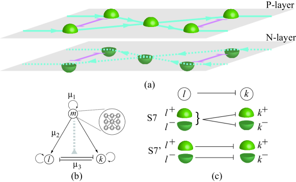
Figure 1: (a) Schematic figure of the network structure of the presented system. Each node consists of a group of oscillators. From (S2), the directional interaction in the N-layer is opposite those in the P-layer. (b) Bidirectional inhibitory links exist at the branching point from (S2). The activation of the inhibitory interaction between nodes $k^{\pm}$ and $l^{\pm}$ is regulated by the state of node $m^{\pm}$. (c) The inhibitory interaction for the current (S7) and previous (S7’) system.

II.1 Equations

The governing equations are as follows:

$$\dot{u}^{j}_{k^{\pm}}=[u^{j}_{k^{\pm}}(1-u^{j}_{k^{\pm}})(u^{j}_{k^{\pm}}-p)-v^{j}_{k^{\pm}}]/\tau_{j}$$ (1)

$$+\mu_{1}F(s_{k^{\pm}};\bar{s})+\mu_{2}\sum_{l^{\pm}\in\Lambda^{\pm}}a_{l^{\pm},k^{\pm}}F(s_{l^{\pm}};\bar{s})+w(t),$$

$$\dot{v}^{j}_{k^{\pm}}=\varepsilon(u^{j}_{k^{\pm}}-qv^{j}_{k^{\pm}}+r)/\tau_{j}$$

$$+\mu_{3}\sum_{m^{\pm}=1^{\pm}}^{K^{\pm}}\sum_{l^{\pm}\in\Lambda^{\pm}}a_{m^{\pm},l^{\pm}}a_{m^{\pm},k^{\pm}}$$

$$\hskip 56.9055pt\times F(s_{m^{\pm},k^{\pm},l^{\pm}};\bar{s})F(s_{l^{\pm}}+\sigma s_{l^{\mp}};\gamma\bar{s})$$

$$s_{k^{\pm}}=\frac{1}{J}\sum_{j=1}^{J}u^{j}_{k^{\pm}},\quad k^{\pm}=1^{\pm},2^{\pm},\dots,K^{\pm},\ j=1,2,\dots,J,$$

where $\Lambda^{\pm}:=\{k\ |\ 1^{\pm}\leq k\leq K^{\pm},k=k^{\mp}\}$, $t$ is dimensionless time, a dot above a variable indicates the derivative of that variable with respect to $t$, and $\mu_{i}$ ($i=1,2,3$) and $\gamma$ are positive constants. The dynamics of each oscillator are described by the FitzHugh-Nagumo equation. $K^{+}$ (or $K^{-}$) is the total number of vertices. From (S4), each node consists of $J$ oscillators and the variables $u_{k}^{j}$ and $v_{k}^{j}$ correspond to the activator and inhibitor, respectively, of the $j$th oscillator in node $k$. The state of each node $k^{\pm}$ is determined by $s_{k^{\pm}}$, the average of $u^{j}_{k^{\pm}}$ ($j=1,2,\dots,J$) in node $k^{\pm}$. The strength of the self-feedback $\mu_{1}$ controls the degree of phase synchronization of the node, where large and small values of $\mu_{1}$ induce synchronization or incoherent oscillation, respectively. Parameters $\mu_{2}$ and $\mu_{3}$ correspond to the strengths of excitatory and inhibitory connections, respectively [Fig.1(b)].

We assume that the interaction function $F$ has a threshold for activation; thus, the state of the connection switches dynamically between the on and off states depending on the state of the node. The regulation of the on-off switching of the connecting nodes depends on $s_{k}$ and is defined by the Heaviside function with a threshold $\bar{s}$, where $F(s_{k};\bar{s})=1$ for $s_{k}>\bar{s}$ and $F(s_{k};\bar{s})=0$ for $s_{k}\leq\bar{s}$. The interactions affect all elements uniformly; that is, they are independent of $j$. The implementation of the Heaviside function is needed to realize condition C3, given later.

Excitatory interaction directed from node $l$ to node $k$ is expressed as $a_{l,k}$, where $a_{l,k}=1$ and $a_{l,k}=0$ indicate the presence and absence of such interactions, respectively. Since the start and goal nodes have a connecting path from the N-layer to the P-layer and a path from the P-layer to the N-layer from (S5), $a_{k_{s}^{-},k_{s}^{+}}=a_{k_{g}^{+},k_{g}^{-}}=1$. It is noted that $a_{k^{\pm},k^{\mp}}=0$ except for $k^{\pm}\not=k_{s}^{\pm}$ and $k^{\pm}\not=k_{g}^{\pm}$ and that $a_{k^{\pm},k^{\pm}}=0$ for all $k^{\pm}$.

From (S2), the system has inhibitory interactions at every branching point of the network (see condition C2). The activation of the inhibitory interaction between nodes $k$ and $l$ is also regulated by $s_{m}$ [Fig.1(b)]. We use the notation $s_{m,k,l}$ to indicate that node $m$ regulates activation of inhibitory interactions between nodes $k$ and $l$.

Assumptions (S7) and (S7’) correspond to the inhibitory functions of the presented system and the previous system, respectively.

• For the presented system, we take $\sigma=1$.

Except for the links at the start and goal nodes, the dynamics of the P-layer and the N-layer are coupled through this inhibitory interaction. From (S7), the inhibitory interactions are activated when $s_{l^{\pm}}+s_{l^{\mp}}$ is larger than $\gamma\bar{s}$ and $s_{m^{\pm}_{,}k^{\pm},l^{\pm}}$ is larger than $\bar{s}$.

To compare the finding time of the presented system with that of the previous system, we use the previous system in Section III. Since the previous system is fundamentally the same as (1) with $\sigma=0$ and $\gamma=1$, we assume (S7’) when we examine numerical experiments of the previous system.

• For the previous system, we take $\sigma=0$ and $\gamma=1$.

We assume (S7) unless otherwise mentioned.

For simplicity, we assume that the parameters $p$, $q$, $r$, and $\varepsilon$ are independent of $k^{\pm}$ and we set $p=0.02$, $q=1.0$, $r=-0.04$, and $\varepsilon=0.01$; $w$ is a small amount of random noise in the interval $[0,0.05]$; the time constants $\tau_{j}$ take random values from the interval between $\tau_{\min}$ and $\tau_{\max}$, where the values of $\tau_{\min}$ and $\tau_{\max}$ are set to $(\tau_{\min},\tau_{\max})=(6.0,6.5)$. The distribution of $\tau_{j}$ is the same for all nodes; that is, it is independent of $k^{\pm}$.

II.2 Regulatory rules

The regulatory rules proposed in ueda are employed for the presented model. Each node can have three qualitatively different states: synchronized oscillation with a large amplitude, synchronized oscillation with a small amplitude, and incoherent oscillation. We refer to these states as large-amplitude synchronized oscillation (LSO), small-amplitude synchronized oscillation (SSO) and incoherent oscillation (INC), respectively. The state LSO means that $s_{k}$ exceeds $\bar{s}$ for every oscillation. The use of the FitzHugh-Nagumo equation admits the presence of SSO when inhibitory interactions are exerted. By regarding LSO as the on state and both SSO and INC as the off state, the proposed system can be regarded as a Boolean network.

The parameter values $\mu_{i}$ are set so that the regulatory rules and the conditions (C1,C2, and C3 in Fig. 2) are satisfied. The parameter values are set to $(\mu_{1},\mu_{2},\mu_{3})=(1.8\times 10^{-3},0.06,0.07)$ and $\bar{s}=0.825$. As discussed later, the state of a node shows INC when no interactions from other nodes are exerted. The value of $\gamma$ is taken from an appropriate regime satisfying the conditions. Here we discuss the regulatory rules for nodes in the P-layer. The same argument can be applied, mutatis mutandis, to the regulatory rules for the nodes in the N-layer.

Since the interactions exert uniformly on the oscillators belonging to the same node, phase resetting of oscillators is observed due to the excitatory interactions. For the given parameter values, the LSO state is propagated along the nodes connected by excitatory links. As shown in Fig.2, the state of node $k^{+}$ becomes LSO when that of node $l^{+}$ is LSO [Fig.2 (C1)]. The node $k^{+}$ becomes INC when the node $l^{+}$ is in one of the off states (SSO or INC) since no interactions are exerted on node $k^{+}$.

At the branching point of excitatory links, we can see the competition between the excitatory and inhibitory interactions. For the inhibitory interactions, the regulatory rules are determined by the states of the node in both layers. The inhibitory interactions from node $k^{\pm}$ to node $l^{\pm}$ become active when both node $k^{+}$ and node $k^{-}$ are in the on state, or $s_{k^{+}}+s_{k^{-}}>\gamma\bar{s}$. Thus, the inhibitory interactions from node $k^{\pm}$ to node $l^{\pm}$ become inactive when either the state of node $k^{+}$ or that of node $k^{-}$ is one of the off states (SSO or INC).

When the state of node $m^{+}$ is LSO, the excitatory interactions are exerted on node $k^{+}$ and node $l^{+}$ from nodes $m^{+}$. In the case that the states of node $l^{-}$ and $l^{+}$ are LSO as shown in Fig.2 (C2)(i), the states of node $k^{+}$ and $k^{-}$ become SSO due to the inhibitory interactions. The role of $k^{+}$ and $l^{+}$ is interchanged when the states of node $k^{+}$ and $k^{-}$ are LSO. In the case that node $l^{-}$ and $k^{-}$ are both in one of the off states, as shown in Fig.2 (C2)(ii) and (iii), the state of nodes $k^{+}$ and $l^{+}$ becomes LSO. When the state of node $m^{+}$ is one of the off states, since $F(s_{m^{+},k^{+},l^{+}})=0$ and the inhibitory interactions are inactive, the nodes $k^{+}$ and $l^{+}$ become INC, independent of the state of the nodes in the N-layer [Fig.2 (C2) (iv) and (v)].

Parameter $\mu_{1}$ is set so that the single node ($\mu_{2}=\mu_{3}=0$) shows transient behavior SSO $\to$ LSO $\to$ INC when SSO is taken as an initial data point (C3). Figure 3 shows the bifurcation diagram of the single node (node $1^{+}$). It is observed that such a state transition from LSO to INC occurs at a limit point, $\mu_{1}\approx 0.006$. By moving $\mu_{1}$ off the limit point of LSO, transient behavior from LSO to INC is observed, and the transition time increases as the distance between $\mu_{1}$ and the limit point becomes smaller. Note that the transient time of LSO becomes longer as the distance from the limiting point becomes smaller. The threshold $\bar{s}$ is taken to be sufficiently large to ensure that the values of $s_{k^{\pm}}$ are smaller than $\bar{s}$, and the state of the node converges to INC when no input is received (see the horizontal dotted line in Fig.3).

In Section III, we can observe that a loop chain of LSO states can be stable due to the regulatory rule (C1). The self-recovery process is established owing to the regulatory rule (C2) with the transient behavior (C3).

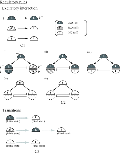
Figure 2: (C1) Regulatory rules for excitatory and inhibitory interactions. (C2) Possible patterns of nodes in the P-layer for the system with (S7) at the branching point of excitatory links. (i) The nodes $k^{+}$ and $k^{-}$ are inhibited when nodes $l^{+}$, $l^{-}$, and $m^{+}$ are in an LSO state. (ii)(iii) The state of node $k^{+}$ and $l^{+}$ becomes LSO when the state of node $m^{+}$ is the on state and nodes $k^{-}$ and $l^{-}$ are in off states (SSO or INC). (iv)(v) The states of nodes $k^{+}$ and $l^{+}$ are INC when node $m^{+}$ is in the off state, independent of the state of nodes in the N-layer. For all patterns, the roles of $k^{+}$ and $l^{+}$ can be interchanged. The possible patterns for the N-layer are given similarly. (C3) Transient behavior when a node receives no input. The solution converges to an INC for any initial condition. Node starting with an SSO approaches a quasi-stable LSO during a finite time interval and finally converges to INC.

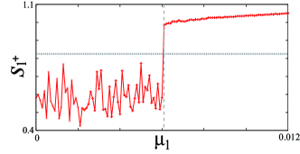
Figure 3: Bifurcation diagram of an isolated node ($\mu_{2}=\mu_{3}=0$). The vertical axis indicates the maximum value of $s_{1^{+}}$. The horizontal dotted line indicates the threshold $\bar{s}$. The limit point is $\mu_{1}\approx 0.006$ (vertical dashed line).

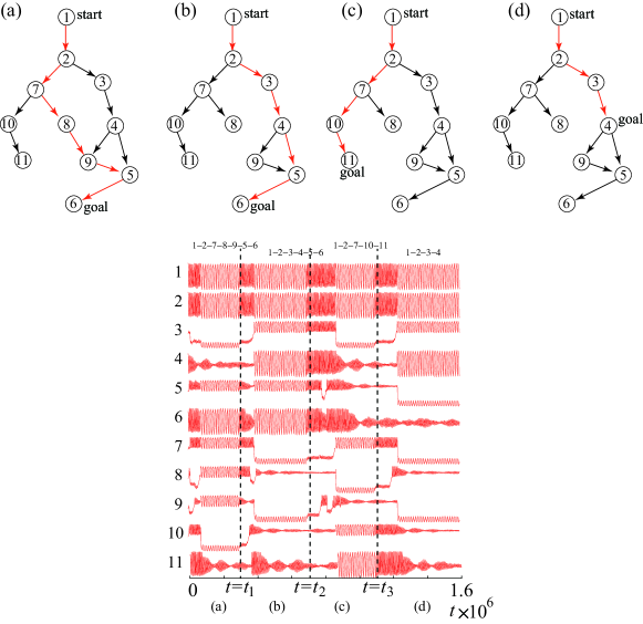
Figure 4: Upper: The graphs used in numerical experiments. Bottom: Time sequences of $s_{k}^{+}$. The sequences of numbers at the top of the figures are the selected vertices. For example, for $t<t_{1}$, vertices 1, 2, 5, 6 7, 8, and 9 are selected.

III Results

In this section, we confirm that the presented system shows the properties (i)-(iii) listed in Section I. A path is defined as a chain of LSO states belonging to the corresponding nodes in both the P-layer and the N-layer. In addition, we demonstrate that the presented system tends to choose shorter paths when multiple paths exist.

III.1 Pathfinding

We test the presented system in the network shown in Fig.4. From (S2), bidirectional inhibitory links are placed between nodes $3^{\pm}-7^{\pm}$, $8^{\pm}-10^{\pm}$, $5^{\pm}-9^{\pm}$, and $4^{\pm}-8^{\pm}$. Initially, we take the start and goal vertices as vertices 1 and 6, respectively; that is, $k_{s}^{\pm}=1^{\pm}$ and $k_{g}^{\pm}=6^{\pm}$ [Fig.4(a)]. At $t=0$, the network has three possible paths connecting the start and goal vertices: path $1\to 2\to 3\to 4\to 5\to 6$, path $1\to 2\to 3\to 4\to 9\to 5\to 6$, and path $1\to 2\to 7\to 8\to 9\to 5\to 6$. In numerical results shown in [Fig.4(a)], path $1\to 2\to 7\to 8\to 9\to 5\to 6$ is selected from the possible paths.

To confirm the self-recovery property, edge 8$\to$9 of the existing edge is removed at $t=t_{1}$ [Fig.4(b)]; the parameter values of $a_{8^{+},9^{+}}$ and $a_{9^{-},8^{-}}$ are changed from $1$ to $0$ at $t=t_{1}$. Then, it is observed that the system can find a new path $1\to 2\to 3\to 4\to 5\to 6$.

The system can find a new path when the positions of the start and goal vertices are changed. For example, in Fig.4(c)(d), it is observed that the system finds a path when the position of the goal vertex is changed from 6 to 11 at $t=t_{2}$ ($a_{6^{+},6^{-}}=0,a_{11^{+},11^{-}}=1$) and from $11$ to $4$ at $t=t_{3}$ ($a_{11^{+},11^{-}}=0,a_{4^{+},4^{-}}=1$). Due to the addition of the excitatory links at $t=t_{3}$, inhibitory links are added between $9^{\pm}-4^{\pm}$ and $5^{\pm}-4^{\pm}$ from (S2) and (S7). When the network has no connecting paths, all of the node states become INC from the regulatory rules.

III.2 Increasing the rate of finding

In order to estimate the increase in the rate of finding as the node number increases, we use a hierarchical tree network, shown in Fig.5: $a_{k+2^{d-1},2k+2^{d}}=a_{k+2^{d-1},2k+1+2^{d}}=1$ ($k=0,1,\dotsc,2^{d-1}-1$, $d=1,2,\dots,d_{\max}$), where $d_{\max}$ is the depth of the hierarchy. The start position is fixed at vertex 1, and the goal vertex is changed between the leftmost vertex (vertex $2^{d_{\max}-1}$) and the rightmost vertex (vertex $2^{d_{\max}}-1$) at the bottom of the tree when the system has succeeded in finding a desired path. For example, in the case of $d_{\max}=2$ (Fig.5), the path contains vertices 1, 2, and 4 when the goal vertex is 4 and vertices 1, 3, and 7 when the goal vertex is 7. The average finding time is calculated across 50 trials.

Now we compare the finding time for the presented system [(S7)] with $\gamma=2$ and the previous system [(S7’)] and $d_{\max}$ are taken as control parameters. In the case of the previous system, the finding time increases substantially as $d_{\max}$ increases [Fig.5 (b)]. In contrast, the finding time increases at an almost constant rate for the presented system.

Next, we investigate the dependence of $\gamma$ on the finding time. It is observed that the finding time is improved and the distributions tend to be narrow when $\gamma$ is increased for $\gamma\leq 2.4$ and $d_{\max}=1,\dotsc,4$. Figure 5 (d) shows the distributions of the finding time when $\gamma$ is taken as a control parameter with $d_{\max}=3$. We note that the distributions tend to be wide again for $\gamma\geq 2.6$. This implies that the large $\gamma$ basically decreases the finding time; however, a large $\gamma$ also decreases the reliability when the vertex number increases.

The difference of the finding time between the two systems comes from the timing of the activation of the inhibitory interaction. The inhibitory interactions play a role in path selection at the branching point of excitatory links. In the presented system, the activation of the inhibitory interaction at node $k^{\pm}$ is regulated by both $s_{k^{+}}$ and $s_{k^{-}}$. This means that the inhibitory interaction for a large $\gamma$ becomes active (i.e., path selection initiates) after an LSO wave propagates to, at least, either the start node or the goal node. In the example network in Fig.6 (a), the path selection initiates after the system succeeds in finding a desired path. This prevents the system from selecting wrong paths, and thus results in a decrease in finding time. In contrast, for the previous system, since the inhibitory interactions activate when either $s_{k^{+}}$ or $s_{k^{-}}$ is larger than $\bar{s}$, the selection of a path at branching points occurs before the system has found both the start and goal vertices, as shown in the example network in Fig.6 (b).

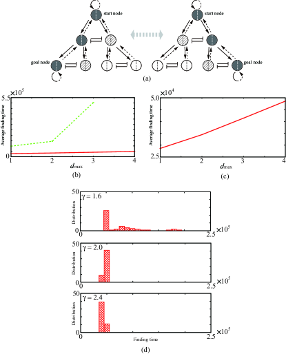
Figure 5: (a) Tree network of depth 2. The left and right halves of the circle indicate nodes in the P-layer and the N-layer, respectively. The solid and dashed lines indicate excitatory links corresponding to the P-layer and the N-layer, respectively. The position of the goal alternates between the two types of networks, changing when the system has succeeded in finding a path. (b) The average finding time of the presented system (solid lines) with $\gamma=2$ and of the previous system (dashed line). (c) Magnified figure of (b). (d) The distribution of finding time of the presented system with $d_{\max}=3$ and $\gamma=1.6,2.0,2.4$.

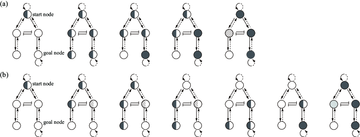
Figure 6: The finding processes of the presented [(a)] and previous [(b)] systems. (a) An LSO wave initially propagates to the wrong path, inhibitory interaction occurs in the second panel from the left, and finally the system converges to the desired solution. (b) Inhibitory interaction occurs after an LSO wave goes through an endpoint (4th panel). The left and right halves of the circle indicate the nodes in the P-layer and the N-layer, respectively.

III.3 Ability of shortest path selection

As discussed in Section III.2, for the presented system, the inhibitory interactions become active when an LSO wave, which has already passed through either the start node or the goal node, first reaches the branching point. Therefore, it is expected that the system chooses a path for which the distance between the branching point and the start or goal node is the shortest; this is, the node distance between the branching point and the start (or goal) node is smallest.

The ratio of the chosen path to the shortest path is calculated for a network shown in Fig.7, where the distance of the path is defined by the number of nodes in the path. The difference of the node number $\Delta$ is taken as a control parameter. As initial data, the state of the start node is set to LSO and the other nodes are set to INC. The number of trials is 100 with different random seeds. It is confirmed that the presented system with $\gamma=2$ and $K^{\pm}=13$ selects shorter paths more frequently as $\Delta$ increases.

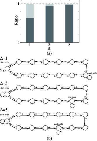
Figure 7: (a) The ratio of success in finding short paths for the network in (b). Black and gray bars indicate the finding ratio of shorter and longer paths for $\Delta=1,3,5$, respectively. (b) Network structures. We fix $K^{\pm}=13$.

IV Discussion

In this study, by building on a previous system ueda , we have presented a pathfinding system. The finding process uses only local interaction between nodes; that is, the presented system is in a class of distributed systems. The system inherits the self-recovery property from the previous system. In fact, we have demonstrated that the system can find a new path when perturbation of the existing paths occurs. We further modify the inhibitory interactions to improve the finding time of the desired path. It has been numerically confirmed that the finding time increases linearly as the depth of the hierarchy of the tree-like network increases.

The self-recovery process is explained by using a network shown in Fig.8. For example, if the goal vertex is changed from $7$ to $4$ [Fig.8(a)], the state of nodes $6^{-}$, $5^{-}$, and $4^{-}$ successively becomes INC due to (C1), and the state of node $2^{\pm}$ is changed from SSO to LSO due to (C3) [Fig.8(b)]. Due to (C1), the state of nodes $3^{+}$, $4^{+}$, $4^{-}$, and $3^{-}$ successively becomes LSO, and the desired path is found [Fig.8(c)(d)]. It should be noted that the LSO state of node $2^{-}$ needs to be maintained during the process (c) to (d). This means that the transient time from LSO to INC should be chosen to be large enough compared to the LSO wave speed and network size by taking $\mu_{1}$ near the limit point in Fig.3.

If the graph contains a cyclic loop that does not contain the start vertex or the goal vertex, the system may fail to find the connecting path between the start and goal nodes, since an LSO loop along the cyclic loop is stable, and the system may choose it. Thus, we assumed (S6).

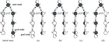
Figure 8: Recovery process when the goal vertex is changed from $7$ to $4$.

References

- (1) D. J. Watts and S. H. Strogatz, Nature 393, 440 (1998).
- (2) W. J. Freeman, R. Kozma, and P. J. Werbos, BioSystems 59, 109 (2001).
- (3) J. J. Hopfield, Proc. Nat. Acad. Sci. 79, 2554 (1982).
- (4) T. Aoyagi, Phys. Rev. Lett. 74, 4075 (1995).
- (5) K. Kunihiko, Physica D: Nonlinear Phenomena 41 137 (1990).
- (6) K. Kaneko, and I. Tsuda, Chaos 13, 926 (2003).
- (7) O. Steinbock, Á. Tóth, and K. Showalter, Science 267, 868 (1995).
- (8) M. Dorigo, G. D. Caro, and L. M. Gambardella, Artificial life 5, 137 (1999).
- (9) T. Nakagaki, H. Yamada, and Á. Tóth, Nature 407, 470 (2000).
- (10) A. Tero, R. Kobayashi, and Toshiyuki Nakagaki, J. theo. Biol. 244, 553 (2007).
- (11) T. Miyaji, and I. Ohnishi, Hokkaido Math. J. 36, 445 (2007).
- (12) K.-I. Ueda, Phys. Rev. E 87 052920 (2013).