Twist-two operators and the BFKL regime
– nonstandard solutions of the Baxter equation

Abstract

The link between BFKL physics and twist-two operators involves an analytical continuation in the spin of the operators away from the physical even integer values. Typically this is done only after obtaining an analytical result for integer spin through nested harmonic sums. In this paper we propose analyticity conditions for the solution of Baxter equation which would work directly for any value of complex spin and reproduce results from the analytical continuation of harmonic sums. We carry out explicit contructions up to 2-loop level. These nonstandard solutions of the Baxter equation have rather surprising asymptotics. We hope that these analyticity conditions may be used for incorporating them into the exact TBA/FiNLIE/QSC approaches valid at any coupling.

1 Introduction

A very important dynamical regime of gauge theory is the Regge limit of high energy scattering characterized by very high energy and fixed momentum transfer (equivalently this corresponds to the small $x$ regime of Deep Inelastic Scattering in QCD). In this regime, scattering amplitudes behave as a power of the energy. A perturbative description at leading order involves a resummation of all terms contributing as $\lambda\log s$ and yields the (LO) BFKL pomeron [1] (and its generalizations to states with more than two reggeized gluons). Currently we know also results at the NLO level both in QCD and in ${\cal N}=4$ SYM [2]. However, there does not seem to be any chance of going directly beyond NLO using only standard perturbative computations.

In the context of ${\cal N}=4$ SYM theory, further progress can be achieved using the methods of the AdS/CFT correspondence. At strong coupling the scattering amplitudes behave like $s^{2}$ (thus the strong coupling pomeron intercept is 2) with the leading contribution coming from graviton exchange [3]. Subsequently, the first correction in $1/\sqrt{\lambda}$ was determined in [4]. Recently, significant progress was made due to the link with twist-2 operators. Indeed, currently we know 3 further terms in the strong coupling expansion of the intercept [5, 6].

BFKL physics is very interesting and important for a number of reasons. Firstly, the pomeron intercept is an example of an IR safe observable relevant for high energy scattering. Secondly, LO BFKL is exactly the same in QCD and in ${\cal N}=4$ SYM. At the NLO level, differences appear, but it would be very interesting to understand completely the conformal physics of the pomeron. On a more theoretical side, the multi-reggeized gluon dynamics at the LO BFKL level in QCD was probably the first place were integrability was discovered in a four dimensional gauge theory. However even now we do not know if, and in what sense, is NLO BFKL integrable. Another fascinating issue is the question how does BFKL fit into our very complete understanding of integrability of the spectral problem in ${\cal N}=4$ SYM. This has to be a very nontrivial link as it is known that even LO BFKL involves an infinite set of wrapping corrections, so any relation between BFKL and AdS/CFT integrability will have to be on the full $AdS_{5}\times S^{5}$ $\sigma$-model level. Even all-loop Asymptotic Bethe Ansatz will not suffice.

Taking all the above into account, it is not clear, however, what is the optimal approach to the study of all-order BFKL physics from the point of view of AdS/CFT integrability. One could either attempt a direct approach dealing with observables directly linked to the pomeron, or a more indirect approach which uses the very close links between BFKL and the anomalous dimensions of twist-2 operators about which we have currently quite detailed knowledge. In this paper we will pursue this latter approach, leaving the more direct approach to a forthcoming paper [7].

The key relation which links the anomalous dimensions of twist-2 operators and the pomeron intercept involves the analytical continuation of these anomalous dimensions away from the physical values of even integer spin $M$. This procedure, which is technically quite demanding, involves finding first an analytical expression for the anomalous dimensions as a function of the spin in terms of so-called nested harmonic sums. Then, one has to find an appropriate analytical continuation of the harmonic sums to arbitrary values of the spin $M$ (and, at weak coupling, analyze the pole structure at $M=-1$).

This procedure, although very involved, has been carried out including Bethe ansatz results [8] and wrapping corrections at 4- [9] and 5-loop level [10]. However, once we would want to study the problem at finite coupling, where we have mainly numerical approaches like TBA (Thermodynamic Bethe Ansatz) [11], FiNLIE (Finite Nonlinear Integral Equations) [12, 13] (and currently the Quantum Spectral Curve (QSC) [14]), this approach is doomed to failure since we cannot perform an analytical continuation from numerical data at integer points.

The motivation for this work is to develop methods for working directly at any complex values of the spin $M$ in a way which is compatible with the known analytical continuations of the nested harmonic sums. Since the basic building block of the spectral problem is a Baxter function (in this context a solution of Baxter equations in the sl(2) sector which should be generalized to the whole T/Y-system once we include arbitrary wrapping corrections), we will propose certain analyticity conditions for the behaviour of the Baxter function for any complex $M$ which would reproduce the analytical continuations of harmonic sums at 1- and 2-loop level. This is the main result of the present paper. We expect, although we do not have a proof, that these analytical conditions should be valid in much more generality. We hope that they can be used in order to formulate a TBA/FiNLIE/QSC problem directly for any complex $M$. Solving these equations would then potentially provide information about BFKL physics valid at any coupling.

The plan of this paper is as follows. In section 2 we will give a brief introduction to the anomalous dimensions of twist-2 operators in the sl(2) sector and state more explicitly their link with BFKL. In section 3 we will review the main properties of 1-loop Baxter equation and in section 4 we will formulate our key proposal for the analytical properties of the physical solution of the Baxter equation at any (non-integer) value of the spin. In section 5 we will explicitly construct the relevant solution of the 1-loop Baxter equation and perform various checks. In section 6 we will show how to extend this solution to the 2-loop level. We close the paper with a summary and outlook and several appendices with some technical details.

2 Twist-two operators and harmonic sums

Twist-two operators in the sl(2) sector are formed out of two complex scalar fields and an arbitrary number $M$ of derivatives ($\equiv$ spin of the operator) along a fixed light-cone direction.

$$O_{M}=\mbox{\rm tr}\,ZD_{+}^{M}Z+\ldots$$ (1)

For each even integer $M$, there appears one new primary state, and its dimension defines the function $\Delta(M)$ for even integer $M$’s. It is known, currently up to 5-loop level [8, 9, 10], that $\Delta(M)$ is expressed in terms of nested harmonic sums. For example up to 2-loop level we have the expression

$$\Delta(M)=2+M+\gamma(M)\equiv 2+M+g^{2}\cdot\gamma^{(1-loop)}(M)+g^{4}\cdot\gamma^{(2-loop)}(M)+\ldots$$ (2)

where

$$\!\!\!\!\gamma^{(1-loop)}(M)\!\!\!\! = \!\!\!\!8\,S_{1}(M)$$

$$\!\!\!\!\gamma^{(2-loop)}(M)\!\!\!\! = \!\!\!\!-16(S_{3}(M)+S_{-3}(M)-2S_{-2,1}(M)+2S_{1}(M)(S_{2}(M)+S_{-2}(M)))$$

These expressions obey the maximal transcendentality principle, which up to now still remains mysterious, which states that the degree of transcendentality of all terms is maximal and equal to $2n-1$, where $n$ is the loop order of the perturbative computation. Even more mysteriously the maximal transcendentality part of the QCD answer exactly coincides with the above expressions for ${\cal N}=4$ SYM.

The harmonic sums are defined as

$$S_{k}(M)=\sum_{j=1}^{M}\frac{1}{j^{k}}\quad\quad S_{k,l}=\sum_{j=1}^{M}\frac{1}{j^{k}}S_{l}(j)$$ (3)

for positive indices, and

$$S_{-k}(M)=\sum_{j=1}^{M}\frac{(-1)^{k}}{j^{k}}\quad\quad S_{-k,l}=\sum_{j=1}^{M}\frac{(-1)^{k}}{j^{k}}S_{l}(j)$$ (4)

for negative (or mixed) indices. These functions have a well defined analytical continuation (such that the only singularities appear on the negative real axis) to complex values of $M$ [15] e.g.

$$S_{1}(M)=\Psi(1+M)-\Psi(1)$$ (5)

but which becomes rapidly more complicated for nested sums and especially for sums with some negative indices (c.f. [15]). In appendix B, we give formulas for the specific harmonic sums that we will use in this paper.

Of particular interest to this paper and its primary motivation is the relation between the anomalous dimensions of twist-2 operators analytically continued to $M=-1+\omega$ and the BFKL pomeron intercept $j(\gamma)$. Indeed the singularities of the anomalous dimension $\gamma$ as a function of $\omega$ can be extracted from the BFKL pomeron intercept through the relation

$$\omega=j(\gamma)-1$$ (6)

The relation between anomalous dimensions and BFKL was first proposed by Jaroszewicz [16], and exploited in [2]. In the ${\cal N}=4$ SYM integrability context it was used by [8] to show explicitly the neccessity of wrapping corrections through a contradiction between Bethe ansatz results at 4-loop level and the BFKL predictions from (6). The inclusion of wrapping corrections, first at 4-loop [9] and then at 5-loop level [10] resolved this contradiction. The above relation between BFKL and twist-2 operators show the neccessity of computing the analytical continuations of the anomalous dimensions of these operators for generic noninteger values of the spin $M$. The investigation of this issue is the main focus of the present paper.

3 Baxter equation in the sl(2) sector

The anomalous dimensions of twist-two operators with even integer spin $M$ can be described using Bethe ansatz with $M$ Bethe roots corresponding to the $M$ excitations, each carrying a unit of spin. As mentioned in the introduction, it is not possible to describe the analytical continuation of these states to noninteger (generally complex) $M$ within this framework. In this paper we will therefore use a standard reformulation of the Bethe ansatz in terms of the Baxter equation, which in fact holds for arbitrary complex $M$.

In the simplest case of 1-loop anomalous dimensions, the Bethe ansatz equations read

$$\left(\frac{u_{j}+\frac{i}{2}}{u_{j}-\frac{i}{2}}\right)^{2}=\prod_{\begin{subarray}{c}k=1\\ k\neq j\end{subarray}}^{M}\frac{u_{k}-u_{j}-i}{u_{k}-u_{j}+i}$$ (7)

while the corresponding Baxter equation takes the form

$$\left(u+i/2\right)^{2}Q(u+i)+\left(u-i/2\right)^{2}Q(u-i)=\underbrace{\left(2u^{2}-M(M+1)-\frac{1}{2}\right)}_{t^{1-loop}(u;M)}Q(u)$$ (8)

If $M$ is integer, then a polynomial solution of (8) is equivalent to (7) with the zeroes of the polynomial $Q(u)$ being identified with the Bethe roots appearing in (7).

Once we relax the condition of integrality of $M$, we have to determine how to pick the physical solution which would coincide with the standard analytical continuation of harmonic sums which determine the energies (anomalous dimensions) and all higher conserved charges of the twist-two states. In the following section we will formulate our proposal for the analyticity conditions which would single out the physical solution for any complex $M$.

In this section we will briefly review some standard properties of the (1-loop) Baxter equation (8). It is clear that the solutions of Baxter equation are determined up to multiplication by an overall periodic function:

$$Q(u)\to f(u)Q(u)\quad\quad\text{with}\quad\quad f(u+i)=f(u)$$ (9)

This is just a gauge symmetry without any physical consequences. A convenient way to factor it out is to introduce the ratio [17]

$$R(u)=\frac{Q(u+i/2)}{Q(u-i/2)}$$ (10)

$R(u)$ also summarizes two infinite sets of conserved charges appearing in its expansion around $u=0$ and $u=\infty$

$$\log R(u)=\sum_{n=1}^{\infty}i\frac{Q_{-n}}{u^{n}}\quad\quad\log R(u)=\sum_{n=1}^{\infty}iQ_{n}u^{n}$$ (11)

Of particular interest for us will be the family of conserved charges with positive indices $Q_{n>0}$ (which include in particular the energy). They are expressed as polynomials of $Q(u)$ and its derivatives evaluated at the special points $u=\pm i/2$. It is convenient to use the normalization $Q(i/2)=1$.

From polynomial solutions of the Baxter equation for even $M$, there are explicit expressions for these derivatives (up to a few first orders) in terms of harmonic sums [18, 19]. In particular we have

$$Q(i/2) = 1\quad\quad\text{(normalization)}$$ (12)

$$Q^{\prime}(i/2) = -2i\,S_{1}$$ (13)

$$Q^{\prime\prime}(i/2) = -4(S_{-2}+S_{1}^{2})$$ (14)

$$Q^{\prime\prime\prime}(i/2) = -24i\left(-2S_{-2,1}-S_{1}S_{-2}-S_{-3}+\frac{1}{3}S_{3}-\frac{1}{3}S_{1}^{3}\right)$$ (15)

The first derivative is just equivalent to the 1-loop energy formula $E=\gamma^{(1-loop)}(M)=8\,S_{1}(M)$. From the above expressions we see that the degree of transcendentality is equal to the order of the derivative. Once we replace the harmonic sums by their standard analytical continuation, we will want to reproduce the above expressions directly from our solution at noninteger $M$.

In addition we have also a closed form expression for all charges $Q_{n>0}$ up to linear order in $M$ [17, 21] which at 1-loop can be conveniently expressed as

$$\log R(u)=\frac{iM}{u}-\frac{iM\sinh(2\pi u)}{2\pi u^{2}}+{\mathcal{O}}\left(M^{2}\right)$$ (16)

This will be again an important cross-check of our solution.

The Baxter equation is a second order difference equation and thus one expects two linearly independent solutions. In fact, once we have a generic (neither even or odd) solution $\tilde{Q}_{1}(u)$, the second solution can be taken to be $\tilde{Q}_{1}(-u)$. However in contrast to the case of second order differential equations, the total space of nonequivalent solutions is in fact infinite dimensional

$$Q(u)=f_{1}(u,M)\tilde{Q}_{1}(u)+f_{2}(u,M)\tilde{Q}_{1}(-u)$$ (17)

with $f_{1}(u,M)$ and $f_{2}(u,M)$ being arbitrary periodic functions with period $i$.

Let us note that there is a well known solution of the Baxter equation valid for arbitrary complex $M$ [22]:

$$\tilde{Q}_{1}(u)={}_{3}F_{2}(-M,M+1,1/2-iu;1,1|1)$$ (18)

In fact this solution reduces to the correct polynomial solution for integer $M$. However it is not the correct physical analytical continuation as it has an explicit $M\to-1-M$ symmetry, which is not a symmetry of the anomalous dimensions $\gamma^{(1-loop)}=8\,S_{1}(M)$. Nevertheless $\tilde{Q}_{1}(u)$ turns out to be a convenient building block of the physical solution as in (17). We will often refer to it as the elementary solution in the following.

Finally, by expanding the Baxter equation at large $u$, one can see that there are two possible large $u$ asymptotics of its solutions:

$$Q(u)\sim u^{M}\quad\quad\text{or}\quad\quad Q(u)\sim u^{-1-M}$$ (19)

This leads to

$$\log R(u)\sim\frac{iM}{u}+{\mathcal{O}}\left(1/u^{2}\right)\quad\quad\text{or}\quad\quad\log R(u)\sim\frac{-i(1+M)}{u}+{\mathcal{O}}\left(1/u^{2}\right)$$ (20)

The first choice reduces to the well known polynomial solutions for integer $M$. Surprisingly, it turns out that it is the other choice which singles out the physical solution for complex $M$.

4 The key proposal

We will now formulate a proposal on the analytical conditions that should single out a particular ‘physical’ solution of the Baxter equation for any complex $M$, such that all physical properties, like anomalous dimensions and higher conserved charges, computed from this solution would coincide with the ones obtained from standard analytical continuation of harmonic sums appearing in the expressions for even integer $M$. We will then proceed to test the above proposal at the 1- and 2-loop level.

Claim: The solution which reproduces all known constraints (BFKL, small $M$ charges) is an even entire function (i.e. with no poles) characterized by the asymptotics

$$\log R(u)\sim\frac{-i(1+M)}{u}+{\mathcal{O}}\left(1/u^{2}\right)$$ (21)

at $u\to\pm\infty$. More precisely, the component of $Q(u)$ with asymptotics $\sim u^{M}$ (which is not modified at higher loop orders) should vanish (or be exponentially suppressed) at $u\to\pm\infty$.

Let us note that this proposal is extremely counterintuitive and unexpected. The above asymptotic condition is in direct contradiction with the physical polynomial solutions at even $M$ which behave at infinity like $u^{M}$. And it is just from these solutions that we get all our information about the energies and charges. It will turn out, however, that the relation between the polynomial solutions and our complex $M$ solution is quite subtle. We will discuss this point at the end of the following section.

5 The 1-loop solution

In this section we will construct the solution of the 1-loop Baxter equation which satisfies the analiticity requirements spelled out in section 4. First we will analyze the pole structure of the elementary solutions and then we will impose the appropriate asymptotics at infinity.

In order to study the properties of the elementary solution $\tilde{Q}_{1}(u)$ it is necessary to have a convergent representation of this function for any $u$. It turns out that the standard power series representation of hypergeometric functions applied to $\tilde{Q}_{1}(u)$ yields

$$\tilde{Q}_{1}(u)=\frac{1}{\Gamma(-M)\Gamma(M+1)\Gamma(1/2-iu)}\sum_{k=0}^{\infty}\frac{\Gamma(k-M)\Gamma(k+M+1)\Gamma(1/2-iu+k)}{k!^{3}}$$ (22)

and gives a valid representation only for $Im\,u<0$. An alternative expression which is valid for $Im\,u>0$ can be obtained using the results and methods of [23]

$$\tilde{Q}_{1}(u) = \frac{\cosh\pi u}{\pi}\frac{\sin^{2}M\pi}{\pi^{2}}\Gamma(1/2-iu)\sum_{k=0}^{\infty}\frac{\Gamma(k-M)\Gamma(k+M+1)\Gamma(1/2+iu+k)}{k!^{3}}\cdot$$ (23)

$$\cdot\left(3\psi(k+1)-\psi(k-M)-\psi(k+M+1)-\psi(1/2+iu+k)\right)$$

Using the above representations, we may derive the behaviour of the elementary solution $\tilde{Q}_{1}(u)$ at $u=\pm i/2$ as these points are crucial for the determination of the energy and higher conserved charges. We find the following behaviour of $\tilde{Q}_{1}(u)$ at $u\sim i/2$:

$$\tilde{Q}_{1}(u)\sim\frac{i\sin M\pi}{\pi(u-i/2)}+\left(\cos M\pi+\frac{2}{\pi}\sin(M\pi)S_{1}(M)\right)+{\mathcal{O}}\left(u-i/2\right)$$ (24)

and at $u\sim-i/2$:

$$\tilde{Q}_{1}(u)\sim\sim 1+{\mathcal{O}}\left(u+i/2\right)$$ (25)

We see that once we move away from integer $M$, a pole appears at $u=i/2$. In order to deal with entire functions we will cancel the poles by multiplying the elementary solutions by an overall periodic function

$$\sinh(2\pi u)\tilde{Q}_{1}(u)\quad\quad\text{and}\quad\quad\sinh(2\pi u)\tilde{Q}_{1}(-u)$$ (26)

One can convince oneself (see appendix A) that the asymptotics of $\tilde{Q}_{1}(u)$ at $u\to+\infty$ are

$$\tilde{Q}_{1}(u)\sim e^{i\pi\frac{M}{2}}\frac{\Gamma(1+2M)}{\Gamma(1+M)^{3}}u^{M}\left(1+\ldots\right)-ie^{-i\pi\frac{M}{2}}\frac{\Gamma(-1-2M)}{\Gamma(-M)^{3}}u^{-1-M}\left(1+\ldots\right)$$ (27)

Asymptotics at $u\to-\infty$ follow by complex conjugation as $\tilde{Q}_{1}(-u)=\tilde{Q}_{1}(u)^{*}$. Hence, if we would like to cancel the $u^{M}$ component in the asymptotics at $u\to\pm\infty$, our solution should reduce to the following combinations of the elementary solutions (up to an overall factor of $\sinh 2\pi u$):

$$u\to+\infty e^{-i\pi\frac{M}{2}}\tilde{Q}_{1}(u)-e^{i\pi\frac{M}{2}}\tilde{Q}_{1}(-u)$$ (28)

$$u\to-\infty e^{i\pi\frac{M}{2}}\tilde{Q}_{1}(u)-e^{-i\pi\frac{M}{2}}\tilde{Q}_{1}(-u)$$ (29)

This shows that the periodic functions appearing in (17) are indeed nontrivial. We will constrain them by the requirement that these functions should not introduce any poles into the solution. An essentially unique minimal choice can be constructed out of constants and $\coth\pi u$ ($\tanh\pi u$ would introduce poles at $u=\pm i/2$, while the poles of $\coth\pi u$ are canceled by the overall factor $\sinh 2\pi u$ which is already in place).

The final 1-loop solution $Q_{1}(u)$ is consequently given by

$$\!\!\!\!\!\frac{\frac{1}{2}i\sinh(2\pi u)}{\sin\pi M}\left[\left(1\!-\!i\,\tan\frac{\pi M}{2}\coth\pi u\right)\tilde{Q}_{1}(u)-\left(1\!+\!i\,\tan\frac{\pi M}{2}\coth\pi u\right)\tilde{Q}_{1}(-u)\right]$$ (30)

Let us comment on some features of the above solution. The overall $M$ dependent factor ensures the normalization

$$Q_{1}(i/2)=1$$ (31)

which is convenient for comparision with the formulas (12)-(15). The solution is even in $u$ for any complex $M$. We checked analytically that $Q_{1}(u)$ reproduces the correct 1-loop energy

$$\gamma^{(1-loop)}(M)=8\,S_{1}(M)$$ (32)

as well as it reproduces all charges at the linear level in $M$:

$$\log R(u)=\frac{iM}{u}-\frac{iM\sinh(2\pi u)}{2\pi u^{2}}+{\mathcal{O}}\left(M^{2}\right)$$ (33)

Furthermore we checked numerically for sample values of $M=-9/10,\,2/3$ and $33/10$ that the formulas (12)-(15) are satisfied to a very high precision. This is a very nontrivial test as e.g. $Q^{\prime\prime\prime}(i/2)$ involves nested harmonic sums of transcendentality 3, some with negative indices, whose analytical continuation is quite intricate (see appendix B for details).

Let us point out that the above mentioned tests were indeed necessary. In fact it is not enough to require only that the 1-loop energy $\gamma^{(1-loop)}(M)=8\,S_{1}(M)$ is recovered in order to single out a unique solution of the Baxter equation. Indeed one can check analytically that the two apparently much simpler solutions

$$\frac{\tilde{Q}_{1}(u)-e^{\pm iM\pi}\tilde{Q}_{1}(-u)}{\sin M\pi}$$ (34)

also give $\gamma^{(1-loop)}(M)=8\,S_{1}(M)$. However they do not agree with what we know about the higher charges in the small $M$ limit. Indeed they have nonzero odd charges and in fact correspond to the two families of charges $q_{n}^{\pm}$ defined in [17] — while the physical solution has charges $\frac{1}{2}(q_{n}^{+}+q_{n}^{-})$.

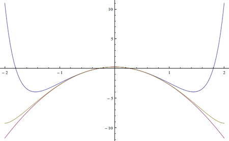
Figure 1: The polynomial solution for $M=2$ (red, bottom curve) and $Q_{1}(u)$ for $M=2.1$ (blue, top curve) and $M=2.01$ (yellow, middle curve)

Finally it remains to discuss the case of integer spin. Then the requirement for our solution, namely its $u^{-M-1}$ asymptotics is in apparent outright contradiction with what we know on the physical polynomial solutions, which in fact were used to derive formulas (12)-(15). How is this possible?

Let us note that the solution $Q_{1}(u)$ defined in (30) behaves in a very nontrivial way when $M$ approaches an integer. In figure 1 we show $Q_{1}(u)$ evaluated numerically for $M=2.1$ and $M=2.01$ and compared it with the standard polynomial solution for $M=2$. We see that the pointwise limit of $Q_{1}(u)$ when $M\to 2$ is the standard polynomial solution. However the limits $u\to\pm\infty$ and $M\to 2$ do not commute and this explains the apparent contradiction. In fact, despite appearances, the solution $Q_{1}(u)$ is not related to the second nonpolynomial solution of the Baxter equation when $M$ is an integer.

6 The 2-loop solution

In this section we will show how to extend the 1-loop solution obtained in the previous section to the 2-loop level.

Here we face a couple of technical difficulties. Although the 2-loop analog of the $\tilde{Q}_{1}(u)$ solution is known explicitly, it is much more difficult to study its analytical properties. Moreover, it will turn out that $\tilde{Q}_{2}(u)$ is more singular at the crucial points $u=\pm i/2$ and we will have to supplant the solution by appropriate choice of $g^{2}$ times a 1-loop solution in order to cancel the poles.

First we will discuss the modifications of the Baxter equation at two loops and then the construction of the solution.

Let us write the Baxter function up to 2-loops as

$$Q(u)=Q_{1}(u)+g^{2}\,Q_{2}(u)+{\mathcal{O}}\left(g^{4}\right)$$ (35)

Then the Baxter equation for $Q_{2}(u)$ is

$$\!\!\!\!\!\!\!\left(u+i/2\right)^{2}Q_{2}(u+i)+\left(u-i/2\right)^{2}Q_{2}(u-i)-t^{1-loop}(u;M)Q_{2}(u)=$$

$$\!\!\!\!\!\!\!=\left(2-i\frac{\gamma^{(1-loop)}}{2}(u+i/2)\right)Q_{1}(u+i)+\left(2+i\frac{\gamma^{(1-loop)}}{2}(u-i/2)\right)Q_{1}(u-i)+$$

$$\!\!\!+\,t^{2-loop}(u;M)\,Q_{1}(u)$$ (36)

where $\gamma^{(1-loop)}(M)=8\,S_{1}(M)$ is the 1-loop energy and

$$t^{2-loop}(u;M)=-\left(4+\frac{2M+1}{2}\gamma^{(1-loop)}\right)$$ (37)

This is the only mild nonlinearity in the dependence of the 2-loop Baxter equation on $Q_{1}(u)$. In [18], a solution of the above equation was found taking $Q_{1}(u)=\tilde{Q}_{1}(u)$. It is given explicitly as

$$\tilde{Q}_{2}(u) = \frac{1}{2}\cdot 8S_{1}(M)\,\frac{\partial}{\partial\delta}\;{}_{3}F_{2}(-M,M+1+2\delta,1/2-iu;1+\delta,1|1)_{|\delta=0}-$$ (38)

$$-\frac{\partial^{2}}{\partial\delta^{2}}\;{}_{3}F_{2}(-M,M+1,1/2-iu;1+\delta,1-\delta|1)_{|\delta=0}-$$

$$-\frac{\partial^{2}}{\partial\delta^{2}}\;{}_{3}F_{2}(-M,M+1,1/2-iu+\delta;1+\delta,1+\delta|1)_{|\delta=0}$$

Hence the nontrivial 2-loop part of $Q_{2}$ corresponding to the physical 1-loop solution (30) is

$$\!\!\!\!\!\frac{\frac{1}{2}i\sinh(2\pi u)}{\sin\pi M}\left[\left(1\!-\!i\,\tan\frac{\pi M}{2}\coth\pi u\right)\tilde{Q}_{2}(u)-\left(1\!+\!i\,\tan\frac{\pi M}{2}\coth\pi u\right)\tilde{Q}_{2}(-u)\right]$$ (39)

We will denote it in what follows by $Q_{2}^{bare}(u)$ in order to emphasize that it is still not the final physical 2-loop solution.

Using the two series representations of hypergeometric functions given in appendix C one can show that $Q_{2}^{bare}(u)$ has second order poles at $u=\pm i/2$. We find explicitly at $u\sim i/2$:

$$Q_{2}^{bare}(u)\sim\frac{2}{(u-i/2)^{2}}-\frac{2i\left(2S_{1}(M)+\pi\tan\frac{M\pi}{2}\right)}{u-i/2}+{\mathcal{O}}\left((u-i/2)^{0}\right)$$ (40)

and at $u\sim-i/2$:

$$Q_{2}^{bare}(u)\sim\frac{2}{(u+i/2)^{2}}+\frac{2i\left(2S_{1}(M)+\pi\tan\frac{M\pi}{2}\right)}{u+i/2}+{\mathcal{O}}\left((u+i/2)^{0}\right)$$ (41)

The leading $2^{nd}$ order poles can be canceled by adding

$$Q_{2}^{bare}(u)\longrightarrow Q_{2}^{bare}(u)-2\pi^{2}\,\tanh^{2}\pi u\,Q_{1}(u)$$ (42)

Of course this modification can be absorbed into a $g$-dependent gauge factor. However the remaining $1^{st}$ order poles have opposite residues at $u=i/2$ and $u=-i/2$ so they cannot be canceled by a periodic function times $Q_{1}(u)$. We can cancel them, however, by a term proportional to $\tilde{Q}_{1}(u)+\tilde{Q}_{1}(-u)$. The asymptotic behaviour of this linear combination has a nonvanishing component proportional to $u^{M}$ — this is allowed by our proposal as other terms are behaving like $\sinh(2\pi u)\cdot u^{-1-M}$, so the $u^{M}$ component is exponentially suppressed in accordance with our key proposal of section 4.

The final form of the 2-loop solution $Q_{2}(u)$ is thus

$$Q_{2}(u)=Q_{2}^{bare}(u)\underbrace{-2\pi^{2}\,\tanh^{2}\pi u\,Q_{1}(u)+\frac{\pi^{2}}{\cos^{2}\frac{M\pi}{2}}(\tilde{Q}_{1}(u)+\tilde{Q}_{1}(-u))}_{\text{necessary to cancel poles}}-c(M)Q_{1}(u)$$ (43)

The final term is added in order to have $Q_{2}(i/2)=0$ which is convenient for comparision with the formulas of [18, 19] analytically continued to arbitrary $M$. The explicit rather complicated expression for $c(M)$ is given in a Mathematica notebook included in the arXiV submission [25].

As a check of the 2-loop solution $Q_{2}(u)$ obtained above, we have numerically evaluated the following expressions [19] for the first and second derivatives at $u=i/2$:

$$Q_{2}(i/2) = 0\quad\quad\text{(normalization)}$$ (44)

$$Q^{\prime}_{2}(i/2) = 8i(S_{3}-S_{-3}+S_{1}(S_{2}+S_{-2})+2S_{2,1})$$ (45)

$$Q^{\prime\prime}_{2}(i/2) = 32S_{-3}S_{1}+32S_{1}^{2}(S_{2}+S_{-2})+32S_{1}S_{3}+$$ (47)

$$+64S_{-3,1}+64S_{-2,2}-128S_{-2,1,1}$$

We found excellent agreement (up to a relative accuracy of at least $10^{-6}$) with the above expressions analytically continued to $M=-9/10,\,2/3$ and $33/10$ using the formulas of appendix B. However, due to the derivatives w.r.t. parameters of the hypergeometric functions appearing in $\tilde{Q}_{2}(u)$ and the nontrivial cancellation of poles exactly at $u=\pm i/2$, a precise numerical evaluation is somewhat involved. We give some details on that in appendix D and attach a Mathematica notebook with that calculation to the arXiV submission [25].

We checked that for sample values of $M$, the behaviour of $Q_{2}(u)/\sinh(2\pi u)$ is decreasing with $u$ (for $u$ up to around $10\sim 12$ and $M=7/3,\,11/3$) in a way which is consistent with the behaviour $1/u^{M+1}(1+c\,\log u)$, however the numerics seem to destabilise for larger $u$ and we cannot reliably fit the exponent $M+1$. But certainly we may rule out the component proportional to $u^{M}$ in accordance with our proposal.

7 Summary and outlook

In this paper we identified asymptotic conditions for a solution of the Baxter equation for twist-2 operators which works for any complex value of the spin. This solution reproduces results such as energies and higher conserved charges which have been previously obtained in the conventional fashion of first finding an analytical expression for the anomalous dimensions for integer spin in terms of nested harmonic sums, and then performing an analytical continuation of these harmonic sums according to the procedure outlined in [15].

The main interest of working directly for complex spin is that in this way we can bypass the stage of finding an analytical expression for integer spin which becomes prohibitively complicated at higher loop level (c.f. the results at 5 loops in [10]) and virtually impossible in the current exact formulations of the spectral problem at any coupling through TBA/FiNLIE/QSC.

The identification of the asymptotic conditions for the Baxter function for any complex spin may aid in constructing a formulation of TBA/FiNLIE/QSC which could be used to study BFKL properties at any coupling. However, one has to note that implementing these conditions in a numerical formulation for $M<-1/2$ may be quite challenging as then, the $u^{M}$ branch becomes subleading at infinity.

There are numerous open problems for further research. Firstly, it would be good to understand the physical justification of the present proposal. The conventional justifications in terms of a construction of a Baxter operator for integrable spin chains [26, 27] would not neccessarily be applicable here, as we even lack a direct hamiltonian construction of the relevant system for complex $M$.

Secondly, it would be very interesting to understand the links with the interrelations between the LO BFKL and anomalous dimensions explored in [28, 29]. These approaches seem to be very different from the present one, especially as some of their formulas become singular in the present setup.

Last but not least, the outstanding open problem would be to implement these conditions as an ingredient of an exact TBA/FiNLIE/QSC formulation valid at any coupling.

Acknowledgments. I would like to thank Zoltan Bajnok for many discussions and Benjamin Basso for various comments. This work was supported by NCN grant 2012/06/A/ST2/00396.

Appendix A Asymptotics of $\tilde{Q}_{1}(u)$

Let us sketch how the asymptotic formula (27) can be motivated. We start from the standard series representation of the hypergeometric function

$$\tilde{Q}_{1}(u)=\frac{1}{\Gamma(-M)\Gamma(M+1)\Gamma(1/2-iu)}\sum_{k=0}^{\infty}\frac{\Gamma(k-M)\Gamma(k+M+1)\Gamma(1/2-iu+k)}{k!^{3}}$$ (48)

We will now use the approximation valid at large $u$:

$$\frac{\Gamma(1/2-iu+k)}{\Gamma(1/2-iu)}\longrightarrow(-iu)^{k}$$ (49)

and substitute it back into the series expression. The series can be summed up to get

$${}_{2}F_{2}(-M,M+1;1,1|-iu)$$ (50)

Now performing a series expansion at $u=\infty$ we get finally the formula

$$\tilde{Q}_{1}(u)\sim e^{i\pi\frac{M}{2}}\frac{\Gamma(1+2M)}{\Gamma(1+M)^{3}}u^{M}\left(1+\ldots\right)-ie^{-i\pi\frac{M}{2}}\frac{\Gamma(-1-2M)}{\Gamma(-M)^{3}}u^{-1-M}\left(1+\ldots\right)$$ (51)

Here we ignored a term proportional to $e^{-iu}$ which is not seen either in a numerical check of (51) which we performed, nor in a related computation using a quite different approach in [23]. This may be an artefact of the approximation (49) which is not entirely reliable as subleading terms at higher orders in $k$ which are discarded are of the same order as lower terms which are kept. We consider it more as heuristics to obtain a formula which we subsequently verify numerically.

Appendix B Harmonic sums — some identities and analytical continuation

In order to reduce the complexity of finding the analytical continuation of nested harmonic sums entering the formulas in [18, 19] we used several identities following from [20]:

$$S_{1,1} = \frac{1}{2}S_{1}^{2}+\frac{1}{2}S_{2}$$

$$S_{1,1,1} = \frac{1}{6}S_{1}^{3}+\frac{1}{2}S_{1}S_{2}+\frac{1}{3}S_{3}$$

$$S_{1,-2} = S_{1}S_{-2}+S_{-3}-S_{-2,1}$$

$$S_{1,-2,1} = -2S_{-2,1,1}+S_{1}S_{-2,1}+S_{-3,1}+S_{-2,2}$$

$$S_{1,2,1} = -2S_{2,1,1}+S_{1}S_{2,1}+S_{3,1}+S_{2,2}$$

$$S_{1,1,-2} = S_{-2,1,1}-S_{1}S_{-2,1}-S_{-3,1}-S_{-2,2}+S_{1}S_{-3}+S_{-4}+\frac{1}{2}S_{-2}(S_{1}^{2}+S_{2})$$

$$S_{1,1,2} = S_{2,1,1}-S_{1}S_{2,1}-S_{3,1}-S_{2,2}+S_{1}S_{3}+S_{4}+\frac{1}{2}S_{2}(S_{1}^{2}+S_{2})$$

$$S_{1,1,1,1} = \frac{1}{4}S_{4}+\frac{1}{8}S_{2}^{2}+\frac{1}{3}S_{1}S_{3}+\frac{1}{4}S_{1}^{2}S_{2}+\frac{1}{24}S_{1}^{4}$$

$$S_{1,-3} = -S_{-3,1}+S_{-3}S_{1}+S_{-4}$$

$$S_{1,3} = -S_{3,1}+S_{1}S_{3}+S_{4}$$

$$S_{2,-2} = -S_{-2,2}+S_{2}S_{-2}+S_{-4}$$

$$S_{2,2} = \frac{1}{2}(S_{2}^{2}+S_{4})$$

$$S_{-2,-2} = \frac{1}{2}(S_{-2}^{2}+S_{4})$$

Below we quote formulas for the analytical continuation of the harmonic sums which appear when evaluating conserved charges for the 1- and 2-loop case. The parameter $a$ in the first two formulas is assumed to be positive.

$$S_{a}(M) = \zeta(a)-\frac{(-1)^{a}}{(a-1)!}\psi_{a-1}(M+1)$$

$$S_{-a}(M) = \zeta(a)(2^{1-a}-1)-\frac{(-1)^{a}}{(a-1)!}\frac{1}{2^{a}}\left(\psi_{a-1}(1+M/2)-\psi_{a-1}((1+M)/2)\right)$$

$$S_{21}(M) = -\frac{5}{8}\zeta(3)+\sum_{m=0}^{\infty}\frac{(-1)^{m}}{(m+M+1)^{2}}\left(\psi(m+M+2)-\psi(1)\right)$$

$$S_{-2,2}(M) = S_{-2,2}(\infty)-\sum_{l=0}^{\infty}\frac{(-1)^{l+1}}{(l+m+1)^{2}}S_{2}(l+M+1)$$

$$S_{-3,1}(M) = S_{-3,1}(\infty)-\sum_{l=0}^{\infty}\frac{(-1)^{l+1}}{(l+m+1)^{3}}S_{1}(l+M+1)$$

$$S_{1,1}(M) = \frac{1}{2}\left(S_{1}(M)^{2}+S_{2}(M)\right)$$

$$S_{-2,1,1}(M) = S_{-2,1,1}(\infty)-\sum_{l=0}^{\infty}\frac{(-1)^{l+1}}{(l+m+1)^{2}}S_{1,1}(l+M+1)$$

Appendix C Properties of $\tilde{Q}_{2}(u)$

In order to analyze the singularity structure of $\tilde{Q}_{2}(u)$ near $u=\pm i/2$ it is neccessary to perform expansions of a more general type of hypergeometric function than the one appearing at 1-loop level, namely

$${}_{3}F_{2}(-M,M+1+2\delta_{1},1/2-iu+\delta_{2};1+\delta_{1}+\delta_{2}+\delta_{3},1+\delta_{2}-\delta_{3}|1)$$ (52)

An expansion in the lower half plane can be obtained directly from the standard definition of the ${}_{3}F_{2}$ similarly as (22). The key difficulty lies in generalizing the representation in the upper half plane (23). The formulas of [23] using representations of Legendre functions are not directly applicable in this case.

The idea of deriving such an expression is to start with the expression

$${}_{3}F_{2}(a,b,\frac{1}{2}-iu+\beta;c,1+\alpha+\beta|1) = \frac{\Gamma(1+\alpha+\beta)}{\Gamma(1/2+iu-\alpha)\Gamma(1/2-iu+\beta)}\cdot$$ (53)

$$\cdot\int_{0}^{1}(1-z)^{iu-\frac{1}{2}+\alpha}z^{-iu-\frac{1}{2}+\beta}{}_{2}F_{1}(a,b;c|z)\,dz$$

which follows directly from power series definitions of the respective functions. Then one expresses ${}_{2}F_{1}(a,b;c|z)$ in terms of ${}_{2}F_{1}(a,b;a+b-c+1|1-z)$ and $(1-z)^{c-a-b}\cdot{}_{2}F_{1}(c-a,c-b;c-a-b+1|1-z)$, and integrates the power series representations term by term. The final expression for ${}_{3}F_{2}(a,b,\frac{1}{2}-iu+\beta;c,1+\alpha+\beta|1)$ is as follows:

$${}_{3}F_{2}(a,b,\frac{1}{2}-iu+\beta;c,1+\alpha+\beta|1)=\frac{\pi\Gamma(c)\Gamma(1+\alpha+\beta)}{\sin\pi(c-a-b)\Gamma(c-a)\Gamma(c-b)\Gamma(a)\Gamma(b)}\bigg{[}$$

$$\sum_{k=0}^{\infty}\frac{\Gamma(a+k)\Gamma(b+k)\Gamma(1/2+\alpha+k+iu)}{\Gamma(a+b-c+1+k)\Gamma(1+\alpha+\beta+k)\Gamma(1/2+\alpha+iu)k!}-$$

$$-\sum_{k=0}^{\infty}\frac{\Gamma(c-a+k)\Gamma(c-b+k)\Gamma(1/2-a+\alpha-b+c+k+iu)}{\Gamma(c-a-b+1+k)\Gamma(1-a+\alpha-b+\beta+c+k)\Gamma(1/2+\alpha+iu)k!}\bigg{]}$$

The above expressions were also neccessary to derive the constant $c(M)$ appearing in our final expression for $Q_{2}(u)$. Since the expression for $c(M)$ is rather complicated, it is given in a Mathematica notebook attached to the arXiV submission [25].

Appendix D Some details on the numerical evaluation of the 2-loop solution

In order to perform numerical checks of the charges of the 2-loop solution we face two main difficulties. Firstly, the elementary 2-loop solution $\tilde{Q}_{2}(u)$ is difficult to evaluate numerically in Mathematica as it involves derivatives of ${}_{3}F_{2}$ w.r.t. parameters of the hypergeometric function. Secondly, we need to evaluate derivatives of $Q_{2}(u)$ at $u=i/2$, where the elementary 2-loop solution has $3^{rd}$ order poles. Of course, these poles will get canceled by the overall factor of $\sinh 2\pi u$ and subtractions of appropriate 1-loop solutions, but a precise numerical evaluation is therefore difficult.

We perform the numerical evaluation in two steps. First we adjust the $c(M)$ coefficient in $Q_{2}(u)$ so that $Q_{2}(\pm i/2)=0$. This is done analytically using series representations of $Q_{2}(u)$ derived in appendix C. Then we construct a Chebyshev grid of 20 points between $u=\pm i/2$. Once we will evalute the values of $Q_{2}$ at the interior points of this grid, we will be able to evaluate very precisely derivatives at $u=i/2$ using Chebyshev differentiation matrix.

It remains thus to evaluate the values of $\tilde{Q}_{2}(u)$ at a number of points in the interior of the interval $(-i/2,i/2)$.

Now each term of $\tilde{Q}_{2}(u)$ is a derivative w.r.t. $\delta$ at $\delta=0$ of a hypergeometric function e.g.

$$\frac{\partial}{\partial\delta}\;{}_{3}F_{2}(-M,M+1+2\delta,1/2-iu;1+\delta,1|1)_{|\delta=0}$$ (54)

For each of these points $u\in(-i/2,i/2)$ we will use a second Chebyshev grid in $\delta$ of 21 points in the interval $(-1/2000,1/2000)$. We will use Mathematica to evaluate the hypergeometric functions for these $\delta$ and use Chebyshev differentiation to extract the derivative w.r.t $\delta$ at $\delta=0$. We attach a Mathematica notebook with this computation to the arXiV submission [25].

References

-
[1]
L. N. Lipatov,
“Reggeization of the vector meson and the
vacuum singularity in nonabelian gauge theories,”
Sov. J. Nucl. Phys. 23 (1976) 338
[Yad. Fiz. 23 (1976) 642];
E. A. Kuraev, L. N. Lipatov and V. S. Fadin, “The Pomeranchuk singularity in nonabelian gauge theories,” Sov. Phys. JETP 45 (1977) 199 [Zh. Eksp. Teor. Fiz. 72 (1977) 377];
I. I. Balitsky and L. N. Lipatov, “The Pomeranchuk singularity in Quantum Chromodynamics,” Sov. J. Nucl. Phys. 28 (1978) 822 [Yad. Fiz. 28 (1978) 1597]. - [2] A. V. Kotikov and L. N. Lipatov, “DGLAP and BFKL equations in the N=4 supersymmetric gauge theory,” Nucl. Phys. B 661 (2003) 19 [Erratum-ibid. B 685 (2004) 405] [hep-ph/0208220].
- [3] R. A. Janik and R. B. Peschanski, “High-energy scattering and the AdS / CFT correspondence,” Nucl. Phys. B 565 (2000) 193 [hep-th/9907177].
- [4] R. C. Brower, J. Polchinski, M. J. Strassler and C. -ITan, “The Pomeron and gauge/string duality,” JHEP 0712 (2007) 005 [hep-th/0603115].
- [5] M. S. Costa, V. Goncalves and J. Penedones, “Conformal Regge theory,” JHEP 1212 (2012) 091 [arXiv:1209.4355 [hep-th]].
- [6] A. V. Kotikov and L. N. Lipatov, “Pomeron in the N=4 supersymmetric gauge model at strong couplings,” Nucl. Phys. B 874 (2013) 889 [arXiv:1301.0882 [hep-th]].
- [7] R. Janik, P. Laskoś-Grabowski, to appear
- [8] A. V. Kotikov, L. N. Lipatov, A. Rej, M. Staudacher and V. N. Velizhanin, “Dressing and wrapping,” J. Stat. Mech. 0710 (2007) P10003 [arXiv:0704.3586 [hep-th]].
- [9] Z. Bajnok, R. A. Janik and T. Lukowski, “Four loop twist two, BFKL, wrapping and strings,” Nucl. Phys. B 816 (2009) 376 [arXiv:0811.4448 [hep-th]].
- [10] T. Lukowski, A. Rej and V. N. Velizhanin, “Five-Loop Anomalous Dimension of Twist-Two Operators,” Nucl. Phys. B 831 (2010) 105 [arXiv:0912.1624 [hep-th]].
-
[11]
N. Gromov, V. Kazakov, A. Kozak, P. Vieira,
“Exact Spectrum of Anomalous Dimensions of Planar Supersymmetric Yang-Mills Theory: TBA and excited states,”
Lett. Math. Phys. 91 (2010) 265,
[arxiv:0902.4458 [hep-th]];
D. Bombardelli, D. Fioravanti, R. Tateo, “Thermodynamic Bethe Ansatz for planar AdS/CFT: A Proposal,” J. Phys. A: Math. Theor. 42 (2009) 375401, [arxiv:0902.3930 [hep-th]];
G. Arutyunov, S. Frolov, “Thermodynamic Bethe Ansatz for the Mirror Model,” JHEP 0905 (2009) 068, [arxiv:0903.0141 [hep-th]]. - [12] N. Gromov, V. Kazakov, S. Leurent and D. Volin, “Solving the AdS/CFT Y-system,” JHEP 1207 (2012) 023 [arXiv:1110.0562 [hep-th]]
- [13] J. Balog and A. Hegedus, “Hybrid-NLIE for the AdS/CFT spectral problem,” JHEP 1208 (2012) 022 [arXiv:1202.3244 [hep-th]].
- [14] N. Gromov, V. Kazakov, S. Leurent and D. Volin, “Quantum spectral curve for ,” arXiv:1305.1939 [hep-th].
- [15] A. V. Kotikov and V. N. Velizhanin, “Analytic continuation of the Mellin moments of deep inelastic structure functions,” hep-ph/0501274.
- [16] T. Jaroszewicz, “Gluonic Regge Singularities And Anomalous Dimensions In QCD,” Phys. Lett. B 116 (1982) 291.
- [17] B. Basso, “Scaling dimensions at small spin in N=4 SYM theory,” arXiv:1205.0054 [hep-th].
- [18] A. V. Kotikov, A. Rej and S. Zieme, “Analytic three-loop Solutions for N=4 SYM Twist Operators,” Nucl. Phys. B 813 (2009) 460 [arXiv:0810.0691 [hep-th]].
- [19] M. Beccaria, A. V. Belitsky, A. V. Kotikov and S. Zieme, “Analytic solution of the multiloop Baxter equation,” Nucl. Phys. B 827 (2010) 565 [arXiv:0908.0520 [hep-th]].
- [20] J. Blumlein and S. Kurth, “Harmonic sums and Mellin transforms up to two loop order,” Phys. Rev. D 60 (1999) 014018 [hep-ph/9810241].
- [21] N. Gromov, “On the Derivation of the Exact Slope Function,” JHEP 1302 (2013) 055 [arXiv:1205.0018 [hep-th]].
- [22] S. E. Derkachov, G. P. Korchemsky and A. N. Manashov, “Evolution equations for quark gluon distributions in multicolor QCD and open spin chains,” Nucl. Phys. B 566 (2000) 203 [hep-ph/9909539].
- [23] H. J. De Vega and L. N. Lipatov, “Interaction of reggeized gluons in the Baxter-Sklyanin representation,” Phys. Rev. D 64 (2001) 114019 [hep-ph/0107225].
- [24] N. Gromov, V. Kazakov, private communication. See also talk by N. Gromov at IGST 2013.
- [25] Mathematica notebook in the source file of the arXiv submission.
- [26] S. E. Derkachov, G. P. Korchemsky and A. N. Manashov, “Separation of variables for the quantum SL(2,R) spin chain,” JHEP 0307 (2003) 047 [hep-th/0210216].
- [27] R. Frassek, T. Lukowski, C. Meneghelli and M. Staudacher, “Baxter Operators and Hamiltonians for ’nearly all’ Integrable Closed gl(n) Spin Chains,” arXiv:1112.3600 [math-ph].
- [28] G. P. Korchemsky, J. Kotanski and A. N. Manashov, “Multi-reggeon compound states and resummed anomalous dimensions in QCD,” Phys. Lett. B 583 (2004) 121 [hep-ph/0306250].
- [29] S. E. Derkachov, G. P. Korchemsky, J. Kotanski and A. N. Manashov, “Noncompact Heisenberg spin magnets from high-energy QCD. 2. Quantization conditions and energy spectrum,” Nucl. Phys. B 645 (2002) 237 [hep-th/0204124].