Geometrical aspects of quantum walks on random two-dimensional structures

Abstract

We study the transport properties of continuous-time quantum walks (CTQW) over finite two-dimensional structures with a given number of randomly placed bonds and with different aspect ratios (AR). Here, we focus on the transport from, say, the left side to the right side of the structure where absorbing sites are placed. We do so by analyzing the long-time average of the survival probability of CTQW. We compare the results to the classical continuous-time random walk case (CTRW). For small AR (landscape configurations) we observe only small differences between the quantum and the classical transport properties, i.e., roughly the same number of bonds is needed to facilitate the transport. However, with increasing AR (portrait configurations) a much larger number of bonds is needed in the CTQW case than in the CTRW case. While for CTRW the number of bonds needed decreases when going from small AR to large AR, for CTRW this number is large for small AR, has a minimum for the square configuration, and increases again for increasing AR. We corroborate our findings for large AR by showing that the corresponding quantum eigenstates are strongly localized in situations in which the transport is facilitated in the CTRW case.

I Introduction

Coherent dynamical processes in complex systems have become popular in different fields of science, ranging from chemistry and statistical physics Mülken and Blumen (2011); van Kampen (1992) to quantum computation Nielsen and Chuang (2010). The systems can be vastly different, say, optical waveguides Lahini et al. (2011); Heinrich et al. (2012), ultracold Rydberg gases Deiglmayr et al. (2006); Westermann et al. (2006); Mülken et al. (2007a); Côté et al. (2006) or carbon nanotube networks Kumar et al. (2005); Snow et al. (2003); Hu et al. (2004). Quantum mechanically as well as classically, transport in these systems takes place over different topologies which can vary from very ordered (regular) lattices to randomly build networks of interacting nodes. Then, an excitation is created at one or more of the nodes: the dynamics of the excitation is then described in the classical (diffusive) case by continuous-time random walks (CTRW) and in the quantum case by continuous-time quantum walks (CTQW) Mülken and Blumen (2011).

In many cases one is interested in the transport through a network, i.e., an excitation is created somewhere in the network and can leave the network at a given set of nodes. The topological influence on the dynamics is then captured in the survival probability of the excitation to remain within the network. Here, we consider the example of a set of $N$ disconnected nodes arranged on two-dimensional lattices of different aspect ratios (AR) to which we randomly add a fixed number of bonds, $B$, between axially nearest-neighboring nodes. This resembles the random two-dimensional lattices of nanotubes whose conductivity properties have been studied experimentally Kumar et al. (2005); Snow et al. (2003); Hu et al. (2004). There, the interest was in the conductivity from, say, the left side of the lattice to the right side.

In order to elucidate the transport properties of such networks, we calculate for each $B$ the long-time behavior (LTB) of the survival probabilities for CTQW and compare them to the ones for CTQW. We define $p_{0.5}^{QW}=B_{0.5}^{QW}/B_{\rm max}$, where $B_{0.5}^{QW}$ is that number of bonds, out of the total number $B_{\rm max}$, which is needed in order for the LTB of the CTQW survival probability to have reached (roughly) the value $0.5$. The corresponding CTRW probability is $p_{0.5}^{RW}$. Clearly, for the same AR, $p_{0.5}^{QW}$ and $p_{0.5}^{RW}$ can be vastly different, as the quantum-mechanical localization of eigenstates may lead to higher $p$-values for CTQW than for CTRW, see also Ref. Leung et al. (2010) for a study of discrete-time quantum walks.

Before continuing with our analysis we mention the obvious connection to percolation theory Stauffer and Aharony (1994); Sahimi (1994). While we focus on the survival probabilities and their decay due to existing connections from left to right, classical bond percolation focusses on the (first) appearance of such a connection. In our case, typically several of these connections are needed in order to reach the values $0.5$ for the LTB of both, CTQW and CTRW. We further focus on the time-independent case where bonds are permanent, i.e., they cannot be removed from the lattice once they are placed. In dynamical percolation, bonds might also be removed, see Ref. Darázs and Kiss (2013); Kollár et al. (2012).

The paper is organized as follows: Section II introduces the general concepts of CTRW and of CTQW. Furthermore, it discusses the trapping model and the different two-dimensional systems considered here. Section III displays our numerical results obtained for lattices with different AR for classical and for quantum mechanical transport. The paper ends in Section IV with our conclusions.

II Transport over random structures

II.1 General considerations

We start by considering both classical and quantum transport over two-dimensional structures consisting of $N_{x}\times N_{y}=N$ nodes. We denote the position of a site by $j=(j_{x},j_{y})$, with $j_{x}=1,\dots,N_{x}$ and $j_{y}=1,\dots,N_{y}$, i.e. $j_{x}$ and $j_{y}$ are integers which label the lattice in the $x$- and the $y$-directions. Several of these nodes get connected by the $B$-bonds distributed over the structure. This procedure leads to a group of clusters of sites. The information about these bonds is encoded in the $N\times N$ connectivity matrix $\bf A$ (see, for instance, Mülken and Blumen (2011)). The non-diagonal elements of $\mathbf{A}$: pertaining to two sites are $-1$ if the sites are connected by one of the $B$-bonds and zero otherwise. The diagonal element of $\mathbf{A}$ corresponding to a particular site is $f$, where $f$ equals the number of $B$-bonds to which the particular site belongs. Now, it is non-negative definite, i.e. all its eigenvalues are positive or zero. When the structure contains no disconnected parts, $\bf A$ has a single vanishing eigenvalue Biswas et al. (2000). In the following we describe the dynamics of purely coherent and of purely incoherent transport by using the CTQW and the CTRW models, respectively Farhi and Gutmann (1998). In both cases, the dynamics depends very much on the topology of the structure, i.e., on $\mathbf{A}$. In a bra-ket notation, an excitation localized at node $j$ will be viewed as being in the state $|j\rangle\equiv|j_{x}\rangle\ \otimes|j_{y}\rangle\equiv|j_{x},j_{y}\rangle$. The states $\{|j\rangle\}$ form an orthonormal basis set. Classically, the transport over unweighted and undirected graphs can be described by CTRW with the transfer matrix $\mathbf{T}=-\gamma\mathbf{A}$ van Kampen (1992); Farhi and Gutmann (1998); Mülken and Blumen (2011); here, for simplicity, we assume equal transition rates $\gamma=1$ for all the nodes.

II.2 CTQW and CTRW

Quantum mechanically, the set of states $\{|j\rangle\}$ spans the whole accessible Hilbert space. The time evolution of an excitation starting at node $|j\rangle$ can be described by the discrete Hamiltonian $\bf H$; Fahri and Guttmann assumed in Farhi and Gutmann (1998) that $\bf H=-\bf T$ which defines the CTQW corresponding to a CTRW with a given transfer matrix $\bf T$.

The CTRW and the CTQW transition probabilities from the state $|j\rangle$ at time $t=0$ to the state $|k\rangle$ at time $t$ read Mülken and Blumen (2011):

$$p_{k,j}(t)=\langle k|\exp{(-\mathbf{T}t)}|j\rangle$$ (1)

and $$\pi_{k,j}(t)=\arrowvert\langle\ k|\exp{(-i\mathbf{H}t)}|\ j\rangle\arrowvert^{2},$$ (2)

respectively, where we assume $\hbar=1$ in Eq.(2).

II.3 The role of absorption

An excitation does not necessarily stay forever in a particular system: it can either decay or get absorbed at certain sites. Since we assume the lifetime of the excitation to be much longer than all the other relevant time scales, we neglect the global radiative decay. However, there are specific nodes where the excitation can get absorbed (trapped). We call these nodes traps and denote their set by $\mathcal{M}$. We also denote by $M$ the number of elements in $\mathcal{M}$ Mülken et al. (2007b). The presence of traps leads to the decay of the probability to find the excitation in the system as a function of time Mülken and Blumen (2011). For a trap-free structure we denote the transfer matrix and the Hamiltonian by $\mathbf{T}_{0}$ and by $\mathbf{H}_{0}$, respectively. We assume the trapping operator $\hat{\mathbf{\Gamma}}$ to be given by a sum over all trap-nodes $|m\rangle=|m_{x},m_{y}\rangle$ Mülken and Blumen (2011, 2010):

$$\hat{\mathbf{\Gamma}}=\sum_{m\in\mathcal{M}}\Gamma_{m}|m\rangle\langle m|.$$ (3)

Then $\bf T$ and $\bf H$ can be written as $\mathbf{T}=\mathbf{T}_{0}-\mathbf{\Gamma}$ and $\mathbf{H}=\mathbf{H}_{0}-i\mathbf{\Gamma}$. In the CTRW case the transfer matrix stays real; then the transition probabilities can be calculated as:

$$p_{k,j}(t)=\sum_{n=1}^{N}e^{-\lambda_{n}t}\langle k|\phi_{n}\rangle\langle\phi_{n}|j\rangle.$$ (4)

In Eq.(4) $\lambda_{n}$ are the (real) eigenvalues $\lambda_{n}$ and the $|\phi_{n}\rangle$ are the eigenstates of $\mathbf{T}$ .

In the quantum mechanical case, $\mathbf{H}$ is non-hermitian and can have up to $N$ complex eigenvalues $E_{n}=\epsilon_{n}-i\gamma_{n}$, ($n=1,\dots,N$). Then the transition probabilities read:

$$\pi_{k,j}(t)=\left|\sum_{n=1}^{N}e^{-i\epsilon_{n}t}e^{-\gamma_{n}t}\langle k|\psi_{n}\rangle\langle\widetilde{\psi}_{n}|j\rangle\right|^{2},$$ (5)

where $|\psi_{n}\rangle$ and $\langle\widetilde{\psi}_{n}|$ are the right and the left eigenstates of $\mathbf{H}$, respectively. Obviously, the imaginary parts $\gamma_{l}$ of $E_{l}$ determine the temporal decay of $\pi_{k,j}(t)$.

II.4 Structures with different aspect ratios

We now turn to specific examples two-dimensional structures with different AR, see Fig. 1. We distinguish the structures by their aspect ratio $N_{y}/N_{x}$; in particular we denote the configurations of lattices with $N_{y}/N_{x}<1$ as “landscapes” and with $N_{y}/N_{x}>1$ as “portraits”; the case $N_{y}/N_{x}=1$ is the square.

As stated above, we start from a set of $N=N_{x}\times N_{y}$ disconnected nodes, to which we randomly add $B$ bonds between nearest neighbor sites. This can be viewed as having bonds occupied with probability $p=B/B_{\rm max}$, with $B_{\rm max}$ being $B_{\rm max}=2N_{x}N_{y}-(N_{x}+N_{y})$. A simply connected component of this graph is called a cluster; every two nodes of such a cluster are connected to each other by at least one unbroken chain of nearest-neighbors bonds.

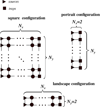
Figure 1: Sketches of structures with square, portrait, and landscape configurations. Here, the triangles denote possible sources and the squares denote the traps (sinks). The $B$-bonds are places on the horizontal and vertical connectivity segments.

We now focus on the transport in the $x$-direction. For this we depict the sites in the first column of the lattice by triangles and call them sources; their coordinates are $|1,l_{y}\rangle$, where $l_{y}=1,\dots,N_{y}$, see Fig. 1. In a similar way, we depict the nodes of the last column by squares and call them traps (sinks). Their coordinates are $|N_{x},m_{y}\rangle$, see Fig.1. Thus, $\hat{\mathbf{\Gamma}}=\sum_{m_{y}=1}^{N_{y}}\Gamma{(|N_{x},m_{y}\rangle\langle m_{y},N_{x}|)}$. Now, a typical process starts by exciting one of the sources. The process gets repeated by exciting another of the sources, and so forth. The classical and the quantum mechanical survival probabilities $P(t)$ and $\Pi(t)$ are now:

$$P(t)=\frac{1}{NN_{y}}\sum_{l_{y},k_{y}=1}^{N_{y}}\sum_{k_{x}=1}^{N_{x}}\langle\ k_{y},k_{x}|e^{-\mathbf{T}t}|1,l_{y}\rangle,$$ (6)

and

$$\Pi(t)=\frac{1}{NN_{y}}\sum_{l_{y},k_{y}=1}^{N_{y}}\sum_{k_{x}=1}^{N_{x}}\arrowvert\langle\ k_{y},k_{x}|e^{-i\mathbf{H}t}|1,l_{y}\rangle\arrowvert^{2}.$$ (7)

Note that in this way $p_{k,j}(t)$ and $\pi_{k,j}(t)$ are averaged over all possible initial states $|1,l_{y}\rangle$ and over all possible final states $|k_{x},k_{y}\rangle$. Furthermore, the time evolution of $p_{k,j}(t)$ and $\pi_{k,j}(t)$ depends on the particular realization of the structure, since for a given, fixed $B$ the distribution of bonds and hence the structure is, in general, random. We evaluate interesting quantities through ensemble averaging over $R=1000$ random structure realisations and set:

$$\langle...\rangle_{R}\equiv\frac{1}{R}\sum_{r=1}^{R}[...]_{r}.$$ (8)

In such a way, we obtain ensemble-averaged survival probabilities $\langle P(t)\rangle_{R}$ and $\langle\Pi(t)\rangle_{R}$ along with their long-time behavior (LTB) $\langle P_{\infty}\rangle_{R}=\lim_{t\to\infty}\langle P(t)\rangle_{R}$ and $\langle\Pi_{\infty}\rangle_{R}=\lim_{t\to\infty}\langle\Pi(t)\rangle_{R}$.

As stressed above, our interest is to determine for which values of $B$ $\langle P_{\infty}\rangle_{R}$ and $\langle\Pi_{\infty}\rangle_{R}$ reach the value $0.5$. We denote these values by $B_{0.5}^{(RW)}$ and $B_{0.5}^{QW)}$, respectively, and obtain thus $p_{0.5}^{(RW)}=B_{0.5}^{(RW)}/B_{\rm max}$ and $p_{0.5}^{(QW)}=B_{0.5}^{(QW)}/B_{\rm max}$.

III Numerical results

III.1 $p_{0.5}^{(RW)}$ for CTRW and $p_{0.5}^{(QW)}$ for CTQW

Figure 2 summarises our findings for the classical $p_{0.5}^{(RW)}$ and for the quantum $p_{0.5}^{(QW)}$ as a function of the AR, namely of $N_{y}/N_{x}$. In general, we find $p_{0.5}^{(QW)}>p_{0.5}^{(RW)}$. For structures with $N_{y}/N_{x}<1$, i.e. in landscape configurations, $p_{0.5}^{(RW)}$ and $p_{0.5}^{(QW)}$ behave quite similarly as a function of $N_{y}/N_{x}$. Now, increasing $N_{y}/N_{x}$ we find that $p_{0.5}^{(RW)}$ has a minimum at $N_{y}/N_{x}\approx 1$, which is not the case for $p_{0.5}^{(QW)}$. For structures with $N_{y}/N_{x}>1$, i.e. in portrait configurations, the behavior of $p_{0.5}^{(RW)}$ and of $p_{0.5}^{(QW)}$ differs with increasing AR: In the CTRW case $p_{0.5}^{(RW)}$ decreases with increasing AR, reflecting the fact that the opposite ends get then closer, so that lower $p$-values are sufficient to ensure on efficient transport. In the CTQW case we find that for $N_{y}/N_{x}>1$ $p_{0.5}^{(QW)}$ increases with increasing AR, a quite counter-intuitive effect which we will discuss in detail in the following.

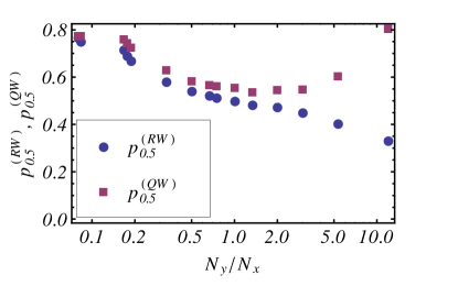
Figure 2: Values of $p_{0.5}^{(RW)}$ and of $p_{0.5}^{(QW)}$ for different AR, $N_{y}/N_{x}$. Note the logarithmic-linear scales.

In Fig. 3 we show particular examples of the $p$-dependence of $\langle P_{\infty}\rangle_{R}$ and $\langle\Pi_{\infty}\rangle_{R}$ for structures with different AR but with roughly the same total number $N$ of nodes. Displayed are:(a) a landscape configuration with $24\times 2$ nodes, (b) a square configuration with $7\times 7$ nodes, and (c) a portrait configuration with $2\times 24$ nodes. One observes as a function of $p$ the transition from states with very inhibited transport, for which $\langle P_{\infty}\rangle_{R}$ and $\langle\Pi_{\infty}\rangle_{R}$ are very close to unity, to states in which the transport is very effective, so that $\langle P_{\infty}\rangle_{R}$ and $\langle\Pi_{\infty}\rangle_{R}$ get very close to zero. From Fig. 3 the values of $p_{0.5}^{(RW)}$ and of $p_{0.5}^{(QW)}$ may be read off. Due to the finite size of the lattices the transition region is rather broad; it gets sharper while increasing $N$. The difference in behavior between $\langle P_{\infty}\rangle_{R}$ and $\langle\Pi_{\infty}\rangle_{R}$ is most evident for the portrait configuration, see Fig. 3(c). Furthermore, in the portrait case the CTRW $\langle P_{\infty}\rangle_{R}$ is smaller than in the square and in the landscape configurations. This is different than for the CTQW case, where $p_{0.5}^{(QW)}$ is larger than in the square and in the landscape configurations.

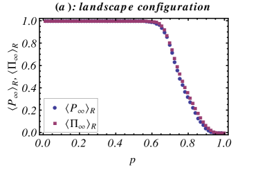
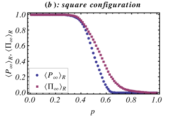
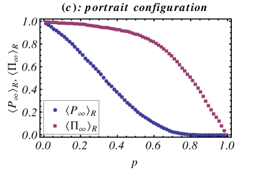
Figure 3: Values of $\langle P_{\infty}\rangle_{R}$ (circles) and of $\langle\Pi_{\infty}\rangle_{R}$ (squares) as a function of $p$ for structures with different aspect ratios but with the same $B$ and roughly the same $N$: (a) a landscape configuration with $24\times 2$ nodes, (b) a square configuration with $7\times 7$ nodes, and (c) a portrait configuration with $2\times 24$ nodes.

In the landscape configuration, the limit $N_{y}/N_{x}\to 0$ leads to the situation of a very long (infinite) chain. In this case already one broken bond is enough to inhibit transport, this is in line with our findings, both in the classical and in the quantum mechanical cases, where we have $p_{0.5}^{(RW)}=p_{0.5}^{(QW)}=1$.

On the other hand, in the limit $N_{y}/N_{x}\to\infty$ one finds that for CTRW only a small number of bonds $B$, i.e., a small probability $p$ is sufficient to cause a drop in $\langle P_{\infty}\rangle_{R}$. This is readily seen in the limit $N_{x}=2$, when a horizontal bond is guaranteed in average when $B$ is around $3$ (one has for $N_{x}=2$ roughly twice as many vertical as horizontal bonds), i.e. for $p\simeq 3/3N_{y}=1/N_{y}$. Such a bond connects a source to a trap and this $p$ value, $p\simeq 1/N_{y}$ tends to zero as $N_{y}/N_{x}\to\infty$.

The picture is not so simple in the CTQW case. Here, the survival probability depends on specific features of the eigenstates $|\psi_{n}\rangle$. If these are localized, transport from one node to the other will be inhibited as in the Anderson localization Anderson (1958). In the next section we will analyze the eigenstates of $\mathbf{H}$ in order to understand the relatively large values of $p_{0.5}^{(QW)}$ compared to $p_{0.5}^{(RW)}$ for lattices with portrait configurations.

III.2 Participation ratio and eigenstates

We recall that the participation ratio $|\langle j|\psi_{n,r}^{(0)}\rangle|^{4}$, where $|\psi_{n,r}^{(0)}\rangle$ is the $n$th eigenstate of the $r$th realization of the $\mathbf{H}_{0}$, is a measure of the localization of the different eigenstates. In order to take the ensemble averaging into account, we introduce

$$\langle\Xi_{j,n}\rangle_{R}=\frac{1}{R}\sum_{r}|\langle j|\psi_{n,r}^{(0)}\rangle|^{4}$$ (9)

as the ensemble averaged participation ratio Mülken et al. (2007).

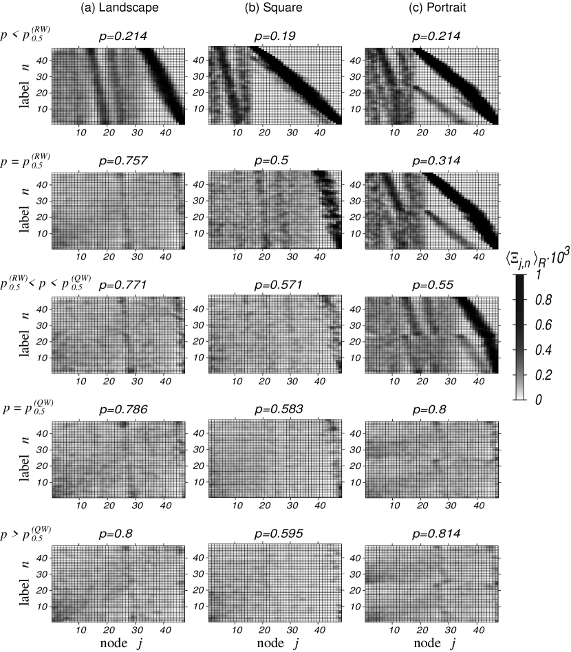
Figure 4: Ensemble averaged participation ratios $\langle\Xi_{j,n}\rangle_{R}$ for different values of $p$, namely $p<p_{0.5}^{(RW)}$, $p=p_{0.5}^{(RW)}$, $p_{0.5}^{(RW)}<p<p_{0.5}^{(QW)}$, $p=p_{0.5}^{(QW)}$, and $p>p_{0.5}^{(QW)}$, for : (a) Landscape configuration for a lattice of $24\times 2$ nodes. (b) Square configuration for a lattice of $7\times 7$ nodes. (c) Portrait configuration for a lattice of $2\times 24$ nodes.

Figure 4 shows in contour plots $\langle\Xi_{j,n}\rangle_{R}$ for lattices whose configuration is (a) landscape, (b) square, and (c) portrait. Here, in each separate panel each row reflects the average contribution of every node $|j\rangle$ of the lattice to a given eigenstate $|\psi_{n,r}\rangle$. In order to see the transition from the situation for $p<p_{0.5}^{(RW)}$ to the one for $p>p_{0.5}^{(QW)}$, we present $\langle\Xi_{j,n}\rangle_{R}$ for distinct $p$ values, namely for $p<p_{0.5}^{(RW)}$, for $p=p_{0.5}^{(RW)}$, for $p_{0.5}^{(RW)}<p<p_{0.5}^{(QW)}$, for $p=p_{0.5}^{(QW)}$, and for $p>p_{0.5}^{(QW)}$. Bright shadings correspond to low while dark shadings correspond to high values of $\langle\Xi_{j,n}\rangle_{R}$. Therefore, localized dark regions indicate localized eigenstates. These, in turn, will inhibit the transport.

This is well in line with the information obtained from Fig. 3, presented in Fig. 3(a) for the landscape configuration. We ramark that, as already noticeable from Fig. 3(a), for the landscape configuration the quantum and the classical $p_{0.5}(t)$-probabilities lie very close together, being $p_{0.5}^{(RW)}=0.757$ and $p_{0.5}^{(QW)}<0.786$. In the depicted case $p_{0.5}^{(RW)}$ and $p_{0.5}^{(QW)}$ differ only by $4\%$, i.e., for $N=48$ only by $2$ bonds in $B_{0.5}$. The eigenstates stray localized up to $p=p_{0.5}^{(QW)}$, see the first panel in Fig. 4(a). For $p>p_{0.5}^{(QW)}$ the eigenstates get more delocalized, which is visible as the grey gets more evenly-distributed over the different nodes $n$.

For the square configuration, Fig. 4(b), the relative difference between $p_{0.5}^{(RW)}$ and $p_{0.5}^{(QW)}$ is about twice as large as for the landscape configuration. Here, one notices a strong localization of the eigenstates for $p$-values up to $p_{0.5}^{(RW)}$, see the first two panels, while this effect is getting less pronounced for larger values of $p$, this already indicates that quantum transport is strongly inhibited for $p$-values below and close to $p_{0.5}^{(RW)}$.

This effect is even more enhanced for the portrait configuration, as may be seen from Fig. 4(c): Up to $p_{0.5}^{(RW)}$ one ramarks very strong localization. This persists even up to $p_{0.5}^{(QW)}=0.8$ which value is more than twice as large as $p_{0.5}^{(RW)}=0.314$. In this particular example one has $N=48$, $B_{0.5}^{(RW)}=22$ and $B_{0.5}^{(RW)}=56$. This means that one needs more than twice more bonds in order to render the quantum transport as efficient as the classical one, in this particular portrait configuration. For smaller $B$ values, the eigenstates are too localized for the quantum transport to be efficient.

IV Conclusions

We have studied the coherent, continuous-time quantum transport on two-dimensional structures of different aspect ratios $N_{y}/N_{x}$ with a given, fixed number $B$ of randomly placed bonds. Having focused on three types of configurations – landscape, square, and portrait – we investigated the long-time probability for an excitation not to get trapped. Our analysis shows that in the average the quantum excitation transport in the $x$-direction becomes very inefficient for structures with portrait configurations, i.e., for those where $N_{y}\gg N_{x}$. This is particularly remarkable, since the opposite holds for (incoherent) continuous-time random walks, where the transport becomes more efficient when the $AR$ increases. This is rendered clear by our evaluations of the classical and quantum mechanical probabilities $p_{0.5}^{(RW)}$ and $p_{0.5}^{(QW)}$ which we have introduced in this article. The behavior in the quantum case can be understood based on an analysis of the corresponding eigenstates. Their participation ratios show that in portrait configurations the eigenstates are still localized for probabilities $p$ such that $p_{0.5}^{(RW)}<p<p_{0.5}^{(RW)}$. Only for $p>p_{0.5}^{(RW)}$ the eigenstates do become delocalized and thus can readily support the transport.

References

- Mülken and Blumen (2011) O. Mülken and A. Blumen, Phys. Rep. 37, 502 (2011).
- van Kampen (1992) N. van Kampen, Stochastic processes in physics and chemistry (Amsterdam: North Holland, 1992).
- Nielsen and Chuang (2010) M. A. Nielsen and I. L. Chuang, Quantum computation and quantum information (Cambridge University Press, 2010).
- Lahini et al. (2011) Y. Lahini, Y. Bromberg, Y. Shechtman, A. Szameit, D. Christodoulides, R. Morandotti, and Y. Silberberg, Phys. Rev. A 84, 041806 (2011).
- Heinrich et al. (2012) M. Heinrich, R. Keil, Y. Lahini, U. Naether, F. Dreisow, A. Tünnermann, S. Nolte, and A. Szameit, New J. Phys. 14, 073026 (2012).
- Deiglmayr et al. (2006) J. Deiglmayr, M. Reetz-Lamour, T. Amthor, S. Westermann, A. De Oliveira, and M. Weidemüller, Opt. Commun. 264, 293 (2006).
- Westermann et al. (2006) S. Westermann, T. Amthor, A. De Oliveira, J. Deiglmayr, M. Reetz-Lamour, and M. Weidemüller, Eur. Phys. J. D 40, 37 (2006).
- Mülken et al. (2007a) O. Mülken, A. Blumen, T. Amthor, C. Giese, M. Reetz-Lamour, and M. Weidemüller, Phys. Rev. Lett. 99, 090601 (2007a).
- Côté et al. (2006) R. Côté, A. Russell, E. E. Eyler, and P. L. Gould, New J. Phys. 8, 156 (2006).
- Kumar et al. (2005) S. Kumar, J. Murthy, and M. Alam, Phys. Rev. Lett. 95, 66802 (2005).
- Snow et al. (2003) E. Snow, J. Novak, P. Campbell, and D. Park, Appl. Phys. Lett. 82, 2145 (2003).
- Hu et al. (2004) L. Hu, D. Hecht, and G. Grüner, Nano Lett. 4, 2513 (2004).
- Leung et al. (2010) G. Leung, P. Knott, J. Bailey, and V. Kendon, New J. Phys. 12, 123018 (2010).
- Stauffer and Aharony (1994) D. Stauffer and A. Aharony, Introduction to percolation theory (CRC, 1994).
- Sahimi (1994) M. Sahimi, Applications of percolation theory (CRC, 1994).
- Darázs and Kiss (2013) Z. Darázs and T. Kiss, J. Phys. A 46, 375305 (2013).
- Kollár et al. (2012) B. Kollár, T. Kiss, J. Novotnỳ, and I. Jex, Phys. Rev. Lett. 108, 230505 (2012).
- Biswas et al. (2000) P. Biswas, R. Kant, and A. Blumen, Macromol. Theor. Simul. 9, 56 (2000).
- Farhi and Gutmann (1998) E. Farhi and S. Gutmann, Phys. Rev. A 58, 915 (1998).
- Mülken et al. (2007b) O. Mülken, V. Bierbaum, and A. Blumen, Phys. Rev. E 75, 031121 (2007b).
- Mülken and Blumen (2010) O. Mülken and A. Blumen, Physica E 42, 576 (2010).
- Anderson (1958) P. W. Anderson, Phys. Rev. 109, 1492 (1958).
- Mülken et al. (2007) O. Mülken, V. Pernice, and A. Blumen, Phys. Rev. E 76, 051125 (2007).