Edge scattering of electrons in graphene

Abstract

We discuss the contribution of edge scattering to the conductance of graphene nanoribbons and nanoflakes. Using different possible types of the boundary conditions for the electron wave function at the edge, we found dependences of the momentum relaxation time and conductance on the geometric sizes and on the carrier density. We also consider the case of ballistic nanoribbon and nanodisc, for which the edge scaterring is the main mechanism of momentum relaxation.

I Introduction

Very unusual transport properties of graphene are mostly related to the electronic energy structure of low-energy states in this material, that can be described by the ultrarelativistic Dirac Hamiltonian. castro09 ; katsnelson The main parameter of this model, electron velocity, does not depend on the electron energy, and is rather high (about $10^{6}$ m/s). Besides, the electron backscattering from impurities is effectively suppressed in graphene (“Klein tunneling” katsnelson ). It results in a rather high mobility of electrons in the graphene bulk despite possible inhomogeneities. Typically, the bulk electron mean-free-path $\ell$ is just several times smaller than the size of graphene flakes $L$ or even comparable with it. This may lead to important contribution of electron scattering from the edges. The main parameter, which determines the condition for essential contribution of the edge scattering, is $\ell/L$. For $\ell/L\ll 1$ the edge scattering leads to a small correction to the transport coefficient but in the opposite (ballistic) case, the edge scattering is the main mechanism of momentum relaxation. Ballistic regime can be experimentally reached for graphene samples. bal1 ; bal2 ; bal3

The effect of electron scattering from the surface has been thoroughly studied in the past for ordinary metals and semiconductors. In the framework of kinetic equation approach, the main problem of the theory is the boundary condition for the electron distribution function at the surface. It was proposed by Fuchs to use a constant specular factor to formulate the boundary condition. fuchs38 It turned out, however, that this approach is too rough to explain numerous experiments. Besides, such boundary condition is not related to any specific mechanism of the surface scattering, and quite obviously does not take into account different character of scattering of electrons incoming under small and large angles to the surface. The problem has been examined in many papers (see, e.g., Refs. [falkovskii70, ; ustinov80, ; peschanskii81, ; katsnelson81, ]) and review articles [okulov79, ; falkovsky83, ] accounting for different scattering mechanisms from different kind of defects, including nonmagnetic and magnetic impurities, surface roughness, etc.

Here we discuss the role of edge scattering in graphene. The essential property of graphene, which makes the results different from the above mentioned results for conventional metallic systems is the behavior of the wave function of electron near the edge. Since the low-energy electrons in graphene are described by relativistic Dirac model, one cannot assume zero wavefunction at the edge, which is the standard way to introduce the metal surface. As a result, the surface scattering vanishes for the sliding electrons with the momentum parallel to the surface, which is especially essential for the ballistic regime $\ell/L\gg 1$. okulov79 ; falkovsky83 The boundary conditions for the wave function in graphene turn out to depend on orientation of the edge with respect to the crystal lattice, on possible edge reconstruction and on the chemical passivation of the edges. katsnelson We will show in this work that it leads, indeed, to an essential difference in the results from those for conventional metals.

Several types of the boundary conditions have been proposed. The so-called Berry-Mondragon berry87 (or infinite-mass) boundary conditions are quite universal to describe the confinement of Dirac electrons in a restricted region as they are not related to the orientation of the boundary. They correspond to the single Dirac cone approximation and therefore are applicable for the case of smooth enough disorder near the edges. It seems to be a good approximation for chemically functionalized edges since the first-principle calculations show that electronic structure is affected at distances much larger than the lattice constant. boukhvalov08

The microscopic model for the boundary conditions and the edge states in graphene, which is based on the real crystallic structure and uses tight-binding approximation, has been considered in several papers. mccann04 ; brey06 ; akhmerov08 ; wimmer10 It was found that for the zigzag boundary, one of the wavefunction components should be necessarily zero at the edge (the other one is zero at the opposite edge). For the armchair boundary it is important to consider two nonequivalent Dirac points (i.e., electrons from different valleys), and the boundary conditions input some phase-dependent relations between the wave functions components of different valleys. It was shown also that for terminated honeycomb lattice zigzag boundary conditions are robust whereas the armchair ones are exceptional. akhmerov08 ; wimmer10 We will focus therefore on two cases, Berry-Mondragon and zigzag edges. In both these cases one can neglect intervalley scattering.

However, the situation with graphene nanoribbons and nanoflakes can be more complicated because of the crystallic reconstruction of the edge, which makes some types of the edges like, e.g., “reczag” reconstruction, energetically more favorable. koskinen08 The boundary conditions for this case has been derived in Ref. [ostaay11, ]. In general, they include the intervalley scattering, which is also relevant for the case of atomically sharp disorder at the edges.

The plan of the paper is the following. In Section II we consider the general solution of the kinetic equation for the graphene nanoribbon, in Section III we derive boundary conditions for the kinetic equation for the nanoribbon with Berry-Mondragon and zigzag boundary conditions, the edge is supposed to be straight line with some defects on it. We will show that the surface scattering vanishes for the sliding electrons in the case of zigzag boundaries but not for the Berry-Mondragon case. In Section IV we calculate the contribution of the edge scattering to the conductance of graphene nanoribbon for $\ell/L\ll 1$. In section V the opposite limit $\ell/L\gg 1$ is considered. In Section VI we consider the scattering by curved edges and in Sections VII and VIII discuss the role of intervalley edge scattering. In Section IX we consider the case of graphene circular flake (nanodisc) with Berry-Mondragon boundary conditions. We finalize with the discussion of the results (Section X) and conclusions (Section XI).

II Formulation of the model for graphene nanoribbon

Let us consider first a narrow graphene ribbon of width $L$ along axis $y$, so that the graphene edges are located at $x=0$ and $x=L$. We assume first that the ribbon edges are ideally flat (straight lines).

The energy spectrum of electrons with momentum ${\bf k}$ and energy $\varepsilon>0$ in the vicinity of $\mathcal{K}$ or $\mathcal{K^{\prime}}$ Dirac points is $\varepsilon(k)=vk$, where $v$ is a constant, and energy $\varepsilon$ is measured from the Dirac point. We assume that graphene is moderately doped, so that the Fermi energy lies at some $\varepsilon_{F}>0$ not far from the Dirac point $\varepsilon=0$.

One can justify the use of the standard semiclassical kinetic equation not too close to the neutrality point, namely, for $k_{F}\ell\gg 1$, where $k_{F}$ is the Fermi wave vector (or, equivalently, when the static conductivity $\sigma\gg e^{2}/h$). katsnelson ; auslender07 Further we will assume this condition to be fulfilled.

The kinetic equation for the stationary distribution function of electrons $f({\bf k},x)=f_{0}+\delta f$ in an electric field $E$ along axis $y$, with $\delta f$ depending on $x$, reads

$$eE\,\frac{\partial f}{\partial k_{y}}+v_{x}\,\frac{\partial f}{\partial x}=-\frac{\delta f}{\tau}\,,$$ (1)

where $f_{0}(\varepsilon)$ is the equilibrium distribution function, $v_{i}=vk_{i}/\hbar k$ is the electron velocity, and $\tau$ is the momentum relaxation time related to the scattering from impurities or other defects in the graphene bulk.

If the external field $E$ is weak, then we use the linear response approximation and obtain from Eq. (1)

$$eEv_{y}\,\frac{\partial f_{0}}{\partial\varepsilon}+v_{x}\,\frac{\partial\delta f}{\partial x}=-\frac{\delta f}{\tau}\,,$$ (2)

where $\varepsilon=v\,(k_{x}^{2}+k_{y}^{2})^{1/2}$. The general solution of Eq. (2) for $v_{x}>0$ and for $v_{x}<0$ can be presented as

$$\delta f^{>}(k_{y},x)=-eEv_{y}\tau\;\frac{\partial f_{0}}{\partial\varepsilon}+\mathcal{C}^{>}(k_{y})\,e^{-x/l_{x}},$$ (3)

$$\delta f^{<}(k_{y},x)=-eEv_{y}\tau\;\frac{\partial f_{0}}{\partial\varepsilon}+\mathcal{C}^{<}(k_{y})\,e^{(x-L)/l_{x}},$$ (4)

respectively, where $l_{x}=|v_{x}|\tau$, and $\mathcal{C}^{>}(k_{y}),\,\mathcal{C}^{<}(k_{y})$ are some arbitrary functions, which have to be found from the boundary conditions at the edges.

It should be noted that the solution (3),(4) is not valid in the limit of $\tau\to\infty$. In such a ballistic limit the functions $\delta f^{>}$ and $\delta f^{<}$ do not depend on $x$, and the electron scattering from the edges should be directly included into the right hand part of the kinetic equation (1) (see below).

III Boundary condition for the distribution function

At the left edge of the ribbon, $x=0$, one can use the following boundary condition for the distribution function

$$|v_{x}|f^{>}(k_{y},0)=|v_{x}|f^{<}(k_{y},0)+\int\frac{d^{2}{\bf k^{\prime}}}{(2\pi)^{2}}\;W_{L}({\bf k},\bf{k^{\prime}})$$

$$\times\left[f^{<}(k^{\prime}_{y},0)-f^{>}(k_{y},0)\right],\hskip 8.5359pt$$ (5)

where $W_{L}({\bf k},{\bf k^{\prime}})$ is the probability of backscattering at the left edge from the state ${\bf k}$ to ${\bf k^{\prime}}$

$$W_{L}({\bf k},{\bf k^{\prime}})=\frac{2\pi N_{i}}{\hbar}\,|\left<{\bf k}|V(x,y)|{\bf k^{\prime}}\right>|^{2}\,\delta(\varepsilon_{{\bf k}}-\varepsilon_{{\bf k^{\prime}}}),$$ (6)

$N_{i}$ is the linear density of scatterers (defects) along the graphene edge, and $V(x,y)$ is the potential of a single scatterer at the edge $x=0$. If there are several different types of scatterers, the probability $W_{L}({\bf k,k^{\prime}})$ is a corresponding sum of several terms (6). The boundary condition (5) accounts for the mirror reflection at the edge and also for reflection from scatterers, which are assumed to be homogenously distributed along the edge.

Analogously, we can write the boundary condition for the distribution function at the right edge of the ribbon, $x=L$

$$|v_{x}|f^{<}(k_{y},L)=|v_{x}|f^{>}(k_{y},L)+\int\frac{d^{2}{\bf k^{\prime}}}{(2\pi)^{2}}\;W_{R}({\bf k},{\bf k^{\prime}})$$

$$\times\left[f^{>}(k^{\prime}_{y},L)-f^{<}(k_{y},L)\right].\hskip 8.5359pt$$ (7)

For simplicity we assume in the following that the type and distribution of impurities and defects is the same at both edges, so that $W_{L}({\bf k},{\bf k^{\prime}})=W_{R}({\bf k},\bf{k^{\prime}})$. It means that in average there is the mirror symmetry $k_{x}\to-k_{x}$.

III.1 Berry-Mondragon boundary condition for the wave function

To calculate the matrix elements of impurity potential $V(x,y)$ in Eq. (6) we should use the wave functions $\left|{\bf k}\right>$ describing the electron states near graphene edge. For this purpose we can write the following Schrödinger equation

$$\left(\begin{array}[]{cc}\varepsilon-\Delta(x)&v(i\partial_{x}+ik_{y})\\ v(i\partial_{x}-ik_{y})&\varepsilon+\Delta(x)\end{array}\right)\left(\begin{array}[]{c}\varphi\\ \chi\end{array}\right)=0,$$ (12)

where $\varphi(x,y)$ and $\chi(x,y)$ are the spinor components of the wave function $\psi(x,y)$, the gap function $\Delta(x)=\Delta_{0}\theta(-x)$, and $\Delta_{0}>>|\varepsilon|$. This corresponds to the vacuum at $x<0$ (with a constant large gap $\Delta_{0}$), and to the graphene at $x>0$, so that the graphene edge is the line $x=0$. The boundary condition of this type has been introduced by Berry and Mondragon.berry87

Using Eq. (8) we find that at $x<0$, $\varphi=Ae^{\kappa_{x}x+ik_{y}y}$ and $\chi=Be^{\kappa_{x}x+ik_{y}y}$, whereas at $x>0$, $\varphi=De^{ik_{x}x+ik_{y}y}$ and $\chi=Fe^{ik_{x}x+ik_{y}y}$. Substituting this to Eq. (8) we find for $x<0$ (vacuum)

$$(\varepsilon-\Delta_{0})A+iv(\kappa_{x}+k_{y})B=0,$$ (13)

$$iv(\kappa_{x}-k_{y})A+(\varepsilon+\Delta_{0})B=0,$$ (14)

and from the condition of zero determinant of the set of linear equations (9),(10) we obtain $\kappa_{x}=\frac{1}{v}(\Delta_{0}^{2}-\varepsilon^{2}+v^{2}k_{y}^{2})^{1/2}\simeq\Delta_{0}/v$. Correspondingly, from (9) and (10) follows $B\simeq-iA$. Due to the continuity of wavefunction at $x=0$ we also obtain $F=-iD=-iA$.

Thus, the wavefunction obeying Berry-Mondragon boundary conditions, near the graphene edge, $x>0$, is

$$\psi_{\bf k}(x,y)=Ae^{i{\bf k}\cdot{\bf r}}\left(\begin{array}[]{c}1\\ -i\end{array}\right),$$ (17)

and the components of wavevector ${\bf k}$ are related by $v(k_{x}^{2}+k_{y}^{2})^{1/2}=\varepsilon$.

We assume that the potential $V(x,y)$, corresponding to a single impurity or defect at the graphene edge, is short ranged in $x$-direction and has a characteristic range $a$ in $y$-direction (i.e., along the edge), so that electron scattering with rather strong $k_{y}$-momentum transfer, $|k_{y}-k^{\prime}_{y}|>1/a$, is effectively suppressed. It corresponds to assumption that the Fourier transform of $y$-dependent random potential does not have wavevector components with $|k_{y}-k^{\prime}_{y}|>1/a$. Such a model can be used to describe different character of the edge scattering of electrons incoming under different angles (diffusive for large angles and nearly specular for small angles).falkovsky83 Hence, one can take $\left<{\bf k}|V(x,y)|{\bf k^{\prime}}\right>\simeq V_{0}e^{-(k_{y}-k^{\prime}_{y})^{2}a^{2}}$, where $V_{0}$ is a constant. Note that it does not matter, in which sublattice A or B of graphene is located the impurity with potential $V(x,y)$.

Then the boundary condition (5) can be written as

$$|v_{x}|f^{>}(k_{y},0)=|v_{x}|f^{<}(k_{y},0)+\frac{2\pi N_{i}V_{0}^{2}}{\hbar}\int\frac{d^{2}{\bf k^{\prime}}}{(2\pi)^{2}}\hskip 14.22636pt$$

$$\times e^{-2(k_{y}-k^{\prime}_{y})^{2}a^{2}}\delta(\varepsilon_{{\bf k}}-\varepsilon_{{\bf k^{\prime}}})\left[f^{<}(k^{\prime}_{y},0)-f^{>}(k_{y},0)\right].\hskip 5.69046pt$$ (18)

We can use

$$\delta(\varepsilon_{{\bf k}}-\varepsilon_{{\bf k^{\prime}}})=\frac{k\,\delta(k^{\prime}_{x}-k^{\prime}_{x0})}{vk^{\prime}_{x}}\,,$$ (19)

where $k^{\prime}_{x0}=(k^{2}-{k^{\prime}_{y}}^{2})^{1/2}$. Then we get from Eq. (12)

$$|v_{x}|f^{>}(k_{y},0)=|v_{x}|\,f^{<}(k_{y},0)+\frac{N_{i}V_{0}^{2}k}{2\pi\hbar v}\hskip 42.67912pt$$

$$\times\int_{-k}^{k}dk^{\prime}_{y}\;e^{-2(k_{y}-k^{\prime}_{y})^{2}a^{2}}\frac{\left[f^{<}(k^{\prime}_{y},0)-f^{>}(k_{y},0)\right]}{(k^{2}-{k^{\prime}_{y}}^{2})^{1/2}}\;,$$ (20)

Assuming that the scattering from impurities at the edge $x=0$ is weak we can substitute $f^{>}(k_{y},0)$ by $f^{<}(k_{y},0)$ in the right-hand part of (14), and we finally present the boundary condition for the distrubution function at $x=0$ as

$$|v_{x}|f^{>}(k_{y},0)=|v_{x}|\,f^{<}(k_{y},0)+\frac{N_{i}V_{0}^{2}k}{2\pi\hbar v}\hskip 42.67912pt$$

$$\times\int_{-k}^{k}dk^{\prime}_{y}\;e^{-2(k_{y}-k^{\prime}_{y})^{2}a^{2}}\frac{\left[f^{<}(k^{\prime}_{y},0)-f^{<}(k_{y},0)\right]}{(k^{2}-{k^{\prime}_{y}}^{2})^{1/2}}\;.$$ (21)

Correspondingly, the second boundary condition for the distribution function at $x=L$ acquires the following form

$$|v_{x}|f^{<}(k_{y},L)=|v_{x}|f^{>}(k_{y},L)+\frac{N_{i}V_{0}^{2}k}{2\pi\hbar v}\hskip 42.67912pt$$

$$\times\int_{-k}^{k}dk^{\prime}_{y}\;e^{-2(k_{y}-k^{\prime}_{y})^{2}a^{2}}\frac{\left[f^{>}(k^{\prime}_{y},L)-f^{>}(k_{y},L)\right]}{(k^{2}-{k^{\prime}_{y}}^{2})^{1/2}}\;.$$ (22)

Substituting Eqs. (3),(4) into Eqs. (15) and (16) we find the solution for the functions $\mathcal{C}_{BM}^{>}(k_{y})$ and $\mathcal{C}_{BM}^{<}(k_{y})$ for the Berry-Mondragon boundary

$$\mathcal{C}^{>}_{BM}(k_{y})=\mathcal{C}^{<}_{BM}(k_{y})=\frac{eE\tau N_{i}V_{0}^{2}}{2\pi\hbar^{2}|v_{x}|\,(1-e^{-L/l_{x}})}\left(-\frac{\partial f_{0}}{\partial\varepsilon}\right)$$

$$\times\int_{-k_{F}-k_{y}}^{k_{F}-k_{y}}\frac{e^{-2q^{2}a^{2}}qdq}{[k_{F}^{2}-(k_{y}+q)^{2}]^{1/2}}\;.\hskip 14.22636pt$$ (23)

This solution is valid for weak disorder at the edge.

III.2 Zigzag boundary condition for the wave function

One can also consider “zigzag” boundary condition for the wavefunction at the left edge, $x=0$, as $\varphi(0)=0$. Its status has been discussed above in the Introduction. Then the wave function at $x>0$ (i.e., in graphene near the edge) has the form

$$\psi_{\bf k}(x,y)\simeq Ae^{ik_{y}y}\left(\begin{array}[]{c}\sin k_{x}x\\ -\frac{ik_{x}}{k}\cos k_{x}x+\frac{ik_{y}}{k}\sin k_{x}x\end{array}\right)$$ (26)

Now the matrix element of impurity potential $V(x,y)$ strongly localized in sublattice A reads

$$\left<{\bf k}|\hat{V}^{(A)}|{\bf k^{\prime}}\right>=|A|^{2}\int d^{2}{\bf r}\,\sin(k_{x}x)\,\sin(k^{\prime}_{x}x)\hskip 14.22636pt$$

$$\times e^{-i(k_{y}-k^{\prime}_{y})y}\,V(x,y)\simeq V_{A}k_{x}k^{\prime}_{x}e^{-(k_{y}-k^{\prime}_{y})^{2}a^{2}},$$ (27)

where $V_{A}$ is a constant.

Analogously, we find for impurity potential localized in sublattice B

$$\left<{\bf k}|\hat{V}^{(B)}|{\bf k^{\prime}}\right>\simeq\frac{|A|^{2}k_{x}k^{\prime}_{x}}{k^{2}}\int d^{2}{\bf r}\,\cos(k_{x}x)\,\cos(k^{\prime}_{x}x)\hskip 14.22636pt$$

$$\times e^{-i(k_{y}-k^{\prime}_{y})y}\,V(x,y)\simeq V_{B}k_{x}k^{\prime}_{x}e^{-(k_{y}-k^{\prime}_{y})^{2}a^{2}},$$ (28)

For the probability of scattering from all such defects located in sublattices A and B at the zigzag boundary we obtain

$$W_{z}({\bf k,k^{\prime}})=\frac{2\pi}{\hbar}\,N_{i}V_{1}^{2}k_{x}^{2}k^{\prime 2}_{x}\,e^{-2(k_{y}-k^{\prime}_{y})^{2}a^{2}}\,\delta(\varepsilon_{\bf k}-\varepsilon_{\bf k^{\prime}}),\hskip 8.5359pt$$ (29)

where we introduced the notation $N_{i}V_{1}^{2}\equiv N_{iA}V_{A}^{2}+N_{iB}V_{B}^{2}$, $N_{iA}$ and $N_{iB}$ are the densities of impurities in sublattices $A$ and $B$, respectively, and $N_{i}$ is the total density of scatterers, $N_{i}=N_{iA}+N_{iB}$. One can assume $N_{iA}\simeq N_{iB}$. We see that in this case (but not for the Berry-Mondragon boundary conditions!) the scattering probability vanishes for the sliding electrons, $k_{x}\rightarrow 0$, similar to the conventional metals.okulov79 ; falkovsky83

Using the same method as before we find for the zigzag boundary

$$\mathcal{C}^{>}_{z}({\bf k})=\mathcal{C}^{<}_{z}({\bf k})=\frac{eE\tau N_{i}V_{1}^{2}k_{x}^{2}}{2\pi\hbar^{2}|v_{x}|\,(1-e^{-L/l_{x}})}\left(-\frac{\partial f_{0}}{\partial\varepsilon}\right)$$

$$\times\int_{-k_{F}-k_{y}}^{k_{F}-k_{y}}e^{-2q^{2}a^{2}}qdq\,[k_{F}^{2}-(k_{y}+q)^{2}]^{1/2},\hskip 5.69046pt$$ (30)

IV Conductance of the graphene nanoribbon

The mean current density in the ribbon can be presented as $j=j_{0}+\delta j$, where the average value is

$$j=\frac{e}{2\pi^{2}vL}\int_{0}^{L}dx\int\varepsilon d\varepsilon\int\frac{k_{y}dk_{y}}{\hbar kk_{x}}\left[\delta f^{>}(k_{y})+\delta f^{<}(k_{y})\right].\hskip 8.5359pt$$ (31)

It includes averaging over the ribbon width. The term $j_{0}$, which does not depend on the edge scattering is

$$j_{0}=\frac{e^{2}E}{\pi^{2}v\hbar}\int\varepsilon d\varepsilon\int\frac{k_{y}dk_{y}}{kk_{x}}\;v_{y}\tau\left(-\frac{\partial f_{0}}{\partial\varepsilon}\right)=\frac{e^{2}E\varepsilon_{F}\tau}{2\pi\hbar^{2}},\hskip 5.69046pt$$ (32)

and $\delta j$ term is due to the edge ($\delta j<0$)

$$\delta j=\frac{e}{\pi^{2}v\hbar L}\int\varepsilon d\varepsilon\int\frac{k_{y}dk_{y}}{kk_{x}}\;l_{x}(1-e^{-L/l_{x}})\,\mathcal{C}^{>}(k_{y}).\hskip 8.5359pt$$ (33)

As follows from (24), $\sigma_{0}=e^{2}\varepsilon_{F}\tau/2\pi\hbar^{2}$ is the conductance of infinite sample, $L\to\infty$.

In the case of Berry-Mondragon boundary conditions, substituting (17) in (25) we obtain

$$\delta j^{(BM)}=j_{0}\,\frac{\tau N_{i}V_{0}^{2}k_{F}}{\pi^{2}v\hbar L}\int_{-1}^{1}\frac{\tilde{k}_{y}d\tilde{k}_{y}}{\sqrt{1-\tilde{k}_{y}^{2}}}$$

$$\times\int_{-1-\tilde{k}_{y}}^{1-\tilde{k}_{y}}\frac{e^{-2\xi\tilde{q}^{2}}\tilde{q}d\tilde{q}}{\sqrt{1-(\tilde{k}_{y}+\tilde{q})^{2}}},$$ (34)

where we denote

$$\xi=a^{2}k_{F}^{2},$$ (35)

$\tilde{k}_{y}=k_{y}/k_{F}$, $\tilde{q}=q/k_{F}$.

In the case of zigzag boundary conditions we get

$$\delta j^{(z)}=j_{0}\,\frac{\tau N_{i}V_{1}^{2}k_{F}^{5}}{\pi^{2}v\hbar L}\int_{-1}^{1}\sqrt{1-\tilde{k}_{y}^{2}}\;\tilde{k}_{y}d\tilde{k}_{y}$$

$$\times\int_{-1-\tilde{k}_{y}}^{1-\tilde{k}_{y}}e^{-2\xi\tilde{q}^{2}}\sqrt{1-(\tilde{k}_{y}+\tilde{q})^{2}}\;\tilde{q}d\tilde{q}.$$ (36)

The dependence of conductivity on  the ribbon width $L$ is shown in Figs. 1 and 2. Here we used

$$\sigma_{BM}=\sigma_{0}\left(1+\frac{\gamma_{BM}\,\ell}{L}\int_{-1}^{1}\frac{\tilde{k}_{y}d\tilde{k}_{y}}{\sqrt{1-\tilde{k}_{y}^{2}}}\right.$$

$$\times\left.\int_{-1-\tilde{k}_{y}}^{1-\tilde{k}_{y}}\frac{e^{-2\xi\tilde{k}_{y}^{2}}\,\tilde{q}d\tilde{q}}{\sqrt{1-(\tilde{k}_{y}+\tilde{q})^{2}}}\right),$$ (37)

$$\sigma_{z}=\sigma_{0}\left(1+\,\frac{\gamma_{z}\,\ell}{L}\int_{-1}^{1}\frac{\tilde{k}_{y}d\tilde{k}_{y}}{\sqrt{1-\tilde{k}_{y}^{2}}}\right.$$

$$\times\left.\int_{-1-\tilde{k}_{y}}^{1-\tilde{k}_{y}}\frac{e^{-2\xi y^{2}}\,\tilde{q}d\tilde{q}}{\sqrt{1-(\tilde{k}_{y}+\tilde{q})^{2}}}\right),$$ (38)

with notations

$$\gamma_{BM}=\frac{N_{i}V_{0}^{2}k_{F}}{\pi^{2}v^{2}},\hskip 8.5359pt\gamma_{z}=\frac{N_{i}V_{1}^{2}k_{F}^{5}}{\pi^{2}v^{2}},\hskip 8.5359pt\ell=\frac{v\tau}{\hbar},$$ (39)

and in Eqs. (29) and (30) $\ell$ is the “bulk” mean path in graphene. Note that Eqs. (29) and (30) are valid only when the second term related to the edge scattering is a small correction to the bulk conductivity, $|\Delta\sigma|\ll\sigma_{0}$.

In numerical calculations of Figs. 1 and 2 we choose the length unit $a_{0}=10^{-8}$ cm. We also take $N_{i}V_{0}^{2}/\pi^{2}v^{2}a_{0}^{2}=10^{2}$ and $N_{i}V_{1}^{2}/\pi^{2}v^{2}a_{0}^{6}=10^{8}$. It corresponds, e.g., to the following choice of parameters: $N_{i}=10^{-4}/a_{0}=10^{4}$ cm^-1, $V_{0}=0.1ta_{0}^{2}\simeq 3\times 10^{-17}$ eV$\cdot$cm², $V_{1}=10^{2}ta_{0}^{4}\simeq 3\times 10^{-30}$ eV$\cdot$cm⁴, $v=10^{-8}$ eV$\cdot$cm. This choice provides fullfillment of the perturbation approximation condition $|\Delta\sigma|\ll\sigma_{0}$. For the $\xi$ parameter we take $\xi=1$ (like for defects in form of ”steps” of the order of electron wave length).

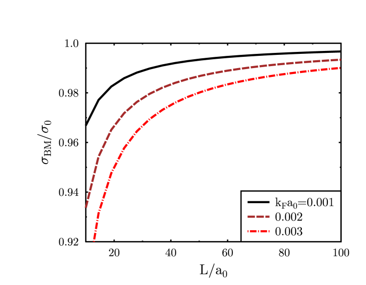
Figure 1: (color online) Conductivity as a function of $L$ for different values of $k_{F}$ (Berry-Mondragon boundary conditions at the edges). For numerical calculations we take $\gamma_{BM}=10^{2}(a_{0}/\ell)(k_{F}a_{0})$.

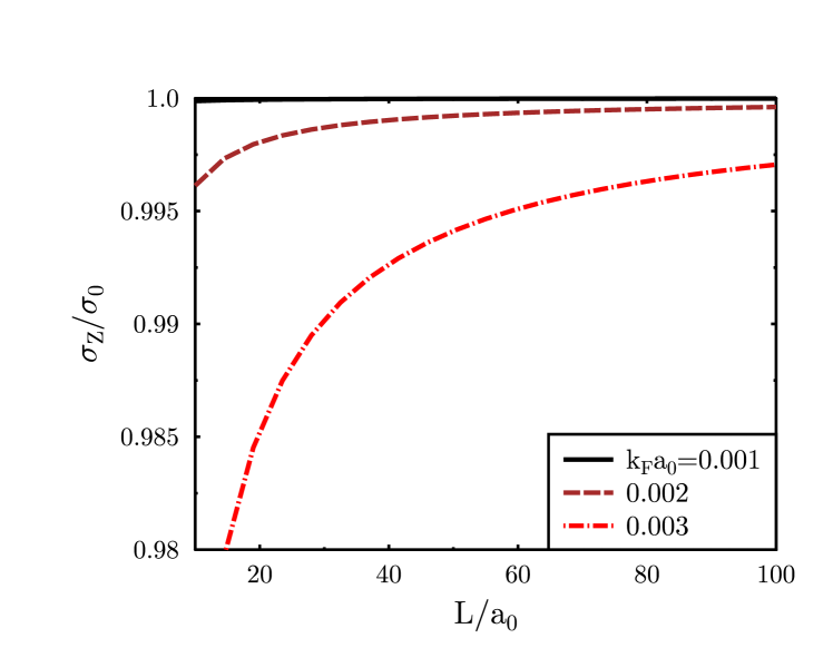
Figure 2: (color online) Conductivity as a function of $L$ for different values of $k_{F}$ (zigzag boundary conditions at the edges). Here we take $\gamma_{z}=10^{8}(a_{0}/\ell)(k_{F}a_{0})^{5}$.

V Graphene nanoribbon in the ballistic regime

Now we assume that there is no scatterers in the bulk. It corresponds to the ballistic limit when the bulk mean free path $\ell$ is large comparing to the ribbon width, $\ell\gg L$. Then the kinetic equation for the distribution function in the bulk includes only the scattering from the edges

$$eEv_{y}\,\frac{\partial f_{0}}{\partial\varepsilon}=\sum_{\bf k^{\prime}}W_{\bf kk^{\prime}}(f^{<,>}_{\bf k^{\prime}}-f^{>,<}_{\bf k})$$ (40)

where $W({\bf k,k^{\prime}})$ is the probability of edge scattering.

Using Eqs. (32) we can decouple them as an equation for $f^{>}_{\bf k}$ and another equation for $f^{<}_{\bf k}$, from which follows that in the ballistic regime $f^{>}_{\bf k}=f^{<}_{\bf k}$. Thus, in this regime we drop out the ”forward” and ”backward” indices. As before, we can find the solutions of these equations by using the boundary condition for the wave function of different type.

V.1 Solution for the Berry-Mondragon boundary

In the case of Berry-Mondragon boundary conditions, Eq. (32) with $f^{>}_{\bf k}=f^{<}_{\bf k}=f_{\bf k}$ can be written as

$$eEv_{y}\,\frac{\partial f_{0}}{\partial\varepsilon}=\frac{2\pi N_{i}V_{0}^{2}}{\hbar L}\int\frac{d^{2}{\bf k^{\prime}}}{(2\pi)^{2}}\;e^{-2(k_{y}-k^{\prime}_{y})^{2}a^{2}}\delta(\varepsilon_{\bf k}-\varepsilon_{\bf k^{\prime}})$$

$$\times\,(f_{\bf k^{\prime}}-f_{\bf k}).\hskip 14.22636pt$$ (41)

The solution of Eq. (33) has the following form

$$f_{\bf k}=eEv_{y}\left(-\frac{\partial f_{0}}{\partial\varepsilon}\right)\tau_{BM}(k_{y}),$$ (42)

where $\tau_{BM}(k_{y})$ is the relaxation time depending on the angle, under which electrons are incoming to the edge, and $\tau_{BM}(k_{y})=\tau_{BM}(-k_{y})$. Substituting Eq. (34) into Eq. (33) we obtain an equation for the function $\tau_{BM}(k_{y})$.

If the parameter $\xi\equiv a^{2}k_{F}^{2}\ll 1$ (which is a realistic case, if $a$ is of the order of several interatomic distances), this equation can be solved analytically. In this case the dependence of $\tau_{BM}$ on $k_{y}$ turns out to be weak. Therefore, the equation for $\tau_{BM}$ reduces to

$$\frac{1}{\tau_{BM}}=-\frac{N_{i}V_{0}^{2}k_{F}}{2\pi\hbar Lv}\,\frac{1}{\tilde{k}_{y}}\int_{-1-\tilde{k}_{y}}^{1-\tilde{k}_{y}}\frac{e^{-2\xi\tilde{q}^{2}}\tilde{q}d\tilde{q}}{\sqrt{1-(\tilde{k}_{y}+\tilde{q})^{2}}}.\hskip 8.5359pt$$ (43)

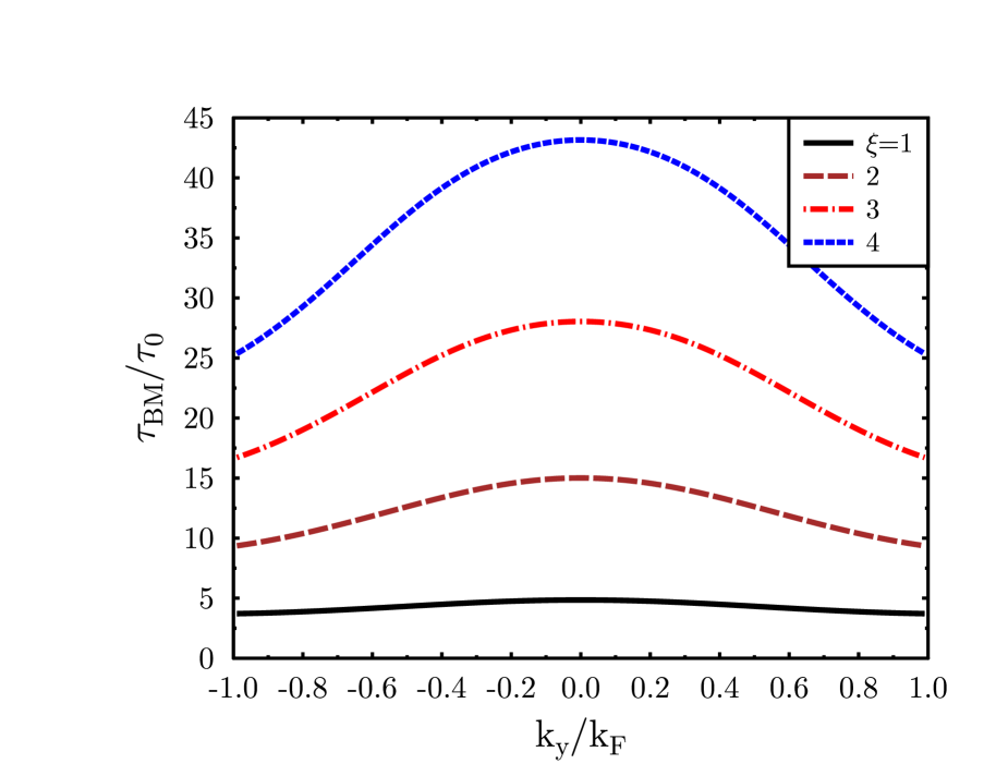
Figure 3: (color online) Relaxation time as a function of $k_{y}/k_{F}$ for different values of the parameter $\xi=a^{2}k_{F}^{2}$ (Berry-Mondragon boundary conditions at the edges).

For arbitrary (not necessarily small) value of the parameter $\xi$ we can present the equation for $\tau_{BM}(k_{y})$ in the following form

$$\int_{-1}^{1}d\tilde{k}^{\prime}_{y}\,e^{-2\xi(\tilde{k}_{y}-\tilde{k}^{\prime}_{y})^{2}}\,\frac{\tilde{k}_{y}\tilde{\tau}_{BM}(\tilde{k}_{y})-\tilde{k}^{\prime}_{y}\tilde{\tau}_{BM}(\tilde{k}^{\prime}_{y})}{\tilde{k}_{y}\tilde{k}^{\prime}_{x}}=1,$$ (44)

where $\tilde{\tau}_{BM}=\tau_{BM}/\tau_{0}$, and $\tau_{0}^{-1}=N_{i}V_{0}^{2}k_{F}/2\pi\hbar Lv$. Thus, we find

$$\tilde{\tau}_{BM}(\tilde{k}_{y})=\frac{1+\int_{-1}^{1}d\tilde{k}^{\prime}_{y}\,e^{-2\xi(\tilde{k}_{y}-\tilde{k}^{\prime}_{y})^{2}}\frac{\tilde{k}_{y}\tilde{\tau}_{BM}(\tilde{k}_{y})}{\tilde{k}_{y}\tilde{k}^{\prime}_{x}}}{\int_{-1}^{1}d\tilde{k}^{\prime}_{y}\,e^{-2\xi(\tilde{k}_{y}-\tilde{k}^{\prime}_{y})^{2}}\frac{1}{\tilde{k}^{\prime}_{x}}}.$$ (45)

Solving Eq. (37) self-consistently by iterations, we find the dependence $\tilde{\tau}_{BM}(\tilde{k}_{y})$. This solution is presented in Fig. 3. It shows that the transport relaxation time of electrons incoming under small angles ($|k_{y}|/k_{F}\sim 1$) is smaller that those incoming under large angles, and this effect is more significant for large $\xi$ (i.e., when the electron wavelength $\lambda$ is small with respect to the characteristic dimension of imperfections, $\lambda\ll a$). In other words, in the case of Berry-Mondragon boundary, sliding electrons are scattered from edges more effectively. This is because the electron wave function is not zero at the edge.

V.2 Solution for the zigzag edge

In the case of zigzag edge, using Eq. (22) and calculating the electron relaxation time like before, for $\xi\ll 1$ we find the solution in the following analytical form

$$\frac{1}{\tau_{z}}=-\frac{N_{i}V_{1}^{2}k_{F}^{5}}{2\pi\hbar Lv}\,\frac{\tilde{k}_{x}^{2}}{\tilde{k}_{y}}\int_{-1-\tilde{k}_{y}}^{1-\tilde{k}_{y}}e^{-2\xi\tilde{q}^{2}}\sqrt{1-(\tilde{k}_{y}+\tilde{q})^{2}}\;\tilde{q}d\tilde{q}.\hskip 5.69046pt$$ (46)

For arbitrary $\xi$ we find the following equation for $\tau_{z}(k_{y})$

$$\tilde{\tau}_{z}(\tilde{k}_{y})=\frac{1+\frac{\tilde{k}_{x}^{2}}{\tilde{k}_{y}}\int_{-1}^{1}d\tilde{k}^{\prime}_{y}\,e^{-2\xi(\tilde{k}_{y}-\tilde{k}^{\prime}_{y})^{2}}\tilde{k}^{\prime}_{y}\tilde{k}^{\prime}_{x}\,\tilde{\tau_{z}}(\tilde{k}^{\prime}_{y})}{\tilde{k}_{x}^{2}\int_{-1}^{1}d\tilde{k}^{\prime}_{y}\,e^{-2\xi(\tilde{k}_{y}-\tilde{k}^{\prime}_{y})^{2}}\tilde{k}^{\prime}_{x}},$$ (47)

where we denote $\tilde{\tau}_{z}=\tau_{z}/\tau_{1}$, and $\tau_{1}^{-1}=N_{i}V_{1}^{2}k_{F}^{5}/2\pi\hbar Lv$.

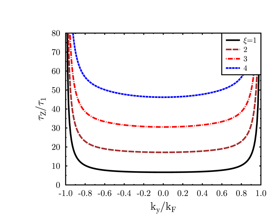
Figure 4: (color online) Relaxation time as a function of $k_{y}/k_{F}$ for different values of the parameter $\xi$ (zigzag boundary conditions at the edges).

Solving Eq. (39) by iteration we find the dependence presented in Fig. 4. As we see, in the case of zigzag boundary, sliding electrons with $|k_{y}|/k_{F}\sim 1$ do not scatter from the edge at any value of the parameter $\xi$. It means that the approximation of constant $\tau_{z}$ and solution (38) are not valid in close vicinity to $|\tilde{k}_{y}|=1$ even for small $\xi$.

V.3 Conductance in ballistic regime

The conductance of carbon nanoribbon can be found now in the case of Berry-Mondragon boundary and for the zigzag edges. We can find, respectively,

$$\sigma_{BM}=\frac{4e^{2}v^{2}L}{N_{i}V_{0}^{2}}\int_{0}^{1}\frac{\tilde{k}_{y}^{2}\,\tilde{\tau}_{BM}(\tilde{k}_{y})\,d\tilde{k}_{y}}{\sqrt{1-\tilde{k}_{y}^{2}}}$$ (48)

where $\tilde{\tau}_{BM}=\tau_{BM}/\tau_{0}$ and

$$\frac{1}{\tilde{\tau}_{BM}(\tilde{k}_{y})}=-\frac{1}{\tilde{k}_{y}}\int_{-1-\tilde{k}_{y}}^{1-\tilde{k}_{y}}\frac{e^{-2\xi\tilde{q}^{2}}\tilde{q}d\tilde{q}}{\sqrt{1-(\tilde{k}_{y}+\tilde{q})^{2}}},$$ (49)

and

$$\sigma_{z}=\frac{4e^{2}v^{2}L}{N_{i}V_{1}^{2}k_{F}^{4}}\int_{0}^{1}\frac{\tilde{k}_{y}^{2}\,\tilde{\tau}_{z}(\tilde{k}_{y})\,d\tilde{k}_{y}}{\sqrt{1-\tilde{k}_{y}^{2}}},$$ (50)

where $\tilde{\tau}_{z}=\tau_{z}/\tau_{1}$ and

$$\frac{1}{\tilde{\tau}_{z}(\tilde{k}_{y})}=-\frac{\tilde{k}_{x}}{\tilde{k}_{y}}\int_{-1-\tilde{k}_{y}}^{1-\tilde{k}_{y}}e^{-2\xi\tilde{q}^{2}}\sqrt{1-(\tilde{k}_{y}+\tilde{q})^{2}}\;\tilde{q}d\tilde{q}.\hskip 8.5359pt$$ (51)

VI Graphene nanoribbon with curved edges

Now we consider the case of curved edges of the ribbon. Let the left edge is now at $x=-L/2+s_{1}(y)$ and the right edge $x=L/2+s_{2}(y)$, where $s_{1}(y)$ and $s_{2}(y)$ are some arbitrary functions characterizing disorder of the ribbon edge. We assume $|s_{1,2}(y)|\ll L$, and disorder properties of $s_{1}(y)$ and $s_{2}(y)$ completely uncorrelated.

It is convenient to introduce new coordinates ($x^{\prime},y^{\prime}$) using conformal transformation

$$x=x^{\prime}+s(y)+\alpha(y)\,x^{\prime},\hskip 14.22636pty=y^{\prime},$$ (52)

where $s(y)=(s_{1}+s_{2})/2$ and $\alpha(y)=(s_{2}-s_{1})/L$. As follows from this definition, each point at the left edge with $x=-L/2+s_{1}(y)$ corresponds to $x^{\prime}=-L/2$, and each point at the right edge with $x=L/2+s_{2}(y)$ corresponds to $x^{\prime}=L/2$. In other words, in new ($x^{\prime},y^{\prime}$) coordinates the edges of ribbon are strait lines.

In correspondance with (44) we find ($|\alpha|\ll 1$)

$$x^{\prime}=\frac{x-s}{1+\alpha}\simeq(x-s)(1-\alpha),\hskip 14.22636pty^{\prime}=y.$$ (53)

The transformation of derivatives is

$$\partial_{x}\simeq(1-\alpha)\,\partial_{x^{\prime}}\,\hskip 8.5359pt\partial_{y}\simeq-s^{\prime}\,\partial_{x^{\prime}}+\partial_{y^{\prime}}\,,$$ (54)

where $s^{\prime}\equiv ds/dy$ and $\alpha^{\prime}\equiv d\alpha/dy$.

The Dirac Hamiltonian in new coordinates is $H=H_{0}+H^{(C)}_{int}$, where $H_{0}=-iv\sigma_{i}\partial_{i}$ and

$$H^{(C)}_{int}=iv\alpha\sigma_{x}\,\partial_{x}+ivs^{\prime}\sigma_{y}\,\partial_{x}$$ (55)

is the perturbation related to the curved edges. As follows from (47) the above-mentioned coordinate transformation generates the following gauge field

$${\bf A}=i\left(\alpha\partial_{x},\;s^{\prime}\partial_{x}\right).$$ (56)

Perturbation (47) leads to nonzero matrix elements of transitions between eigenstates ($k_{x},k_{y}$) and ($k_{x},k^{\prime}_{y}$) of the Hamiltonian $H_{0}$. Due to elasticity of scattering we should take into account only backscattering transitions with $k_{y}\to-k_{y}$, which contribute to the transport properties of graphene nanoribbon.

Matrix elements of transition ${\bf k}\to{\bf k+q}$ with ${\bf q}=(0,\,q)$, are (here we use Berry-Mondragon condition for the wavefunction)

$$\left<{\bf k}|H^{(C)}_{int}|{\bf k+q}\right>=-\frac{\alpha_{q}vk_{x}k_{-}}{k\mathcal{L}}\,,$$ (57)

where $\alpha_{q}=\int\alpha(y)\,e^{-iqy}dy$ and $\mathcal{L}$ is the ribbon length.

Now the right-hand part of kinetic equation is

$${\rm St}\,f_{\bf k}=-\frac{2\pi}{\hbar}\sum_{\bf k^{\prime}}\left|\left<{\bf k}|H^{(C)}_{int}|{\bf k^{\prime}}\right>\right|^{2}\delta(\varepsilon_{\bf k}-\varepsilon_{\bf k^{\prime}})(f_{\bf k}-f_{\bf k^{\prime}})$$

$$=-\frac{|\alpha_{2k_{y}}|^{2}vk_{x}^{2}k}{\hbar k_{y}\mathcal{L}}\,(f_{\bf k}-f_{\bf k+q_{0}}).\hskip 8.5359pt$$ (58)

Here $f_{\bf k}=f(k_{x},k_{y})$ and $f_{\bf k+q_{0}}=f(k_{x},-k_{y})$.

Averaging over realizations of $\alpha(y)$ gives us

$$\overline{|\alpha_{q}|^{2}}=\int dy\,dy^{\prime}\,e^{iq(y-y^{\prime})}\,\overline{\alpha(y)\,\alpha(y^{\prime})}=\mathcal{L}\,C_{q}\,,$$ (59)

where we denote $C_{q}=\int dy\,e^{iqy}\,\overline{\alpha(y)\,\alpha(0)}$. In the following we can assume $C_{q}=\left<\alpha^{2}\right>a_{\alpha}\exp{(-a_{\alpha}^{2}q^{2})}$, where $a_{\alpha}$ is the characteristic length of fluctuations.

Then after averaging we obtain

$${\rm St}\,f_{\bf k}=-\frac{C_{2k_{y}}vk_{x}^{2}k}{\hbar k_{y}}\,(f_{\bf k}-f_{\bf k+q_{0}}),\hskip 8.5359pt$$ (60)

and the kinetic equation acquires the form

$$eEv_{y}\,\frac{\partial f_{0}}{\partial\varepsilon}=-\frac{C_{2k_{y}}vk_{x}^{2}k}{\hbar k_{y}}\,(f_{\bf k}-f_{\bf k+q_{0}}).\hskip 8.5359pt$$ (61)

Hence, one can identify the relaxation time as $\tau_{\bf k}^{-1}=C_{2k_{y}}vk_{x}^{2}k/\hbar k_{y}$.

Electric current along the ribbon is

$$j=\frac{2ev}{\hbar}\int\frac{d^{2}{\bf k}}{(2\pi)^{2}}\frac{k_{y}}{k}\,f_{\bf k}\simeq\frac{e}{2\pi^{2}\hbar v}\int_{0}^{\infty}\frac{k_{y}dk_{y}}{kk_{x}}$$

$$\times\int\varepsilon d\varepsilon\,(f_{\bf k}-f_{\bf k+q_{0}}).$$ (62)

Using (53) and (54) we find the conductance determined by the curved edges

$$\sigma_{C}=\frac{e\varepsilon_{F}}{2\pi^{2}v\hbar}\int_{0}^{k_{F}}\frac{k_{y}dk_{y}}{kk_{x}}\,\frac{ev_{y}\hbar k_{y}}{C_{2k_{y}}vk_{x}^{2}k}=\frac{e^{2}\varepsilon_{F}L}{4\pi^{2}v\hbar k_{F}C_{2k_{F}}}\,,\hskip 5.69046pt$$ (63)

where we have to cut integral at small $k_{x}$ by $k_{min}\simeq 1/L$.

Combining $\sigma_{C}$ with the conductivity of graphene without curved edges $\sigma_{0}$ and assuming $\sigma_{C}\gg\sigma_{0}$ we obtain

$$\sigma\simeq\sigma_{0}\,(1-\sigma_{0}/\sigma_{C}).$$ (64)

Then using Eq. (55) we get

$$\sigma\simeq\sigma_{0}\left(1-\frac{\pi\tau vk_{F}}{\hbar L}\left<\alpha^{2}\right>a_{\alpha}e^{-4a_{\alpha}^{2}k_{F}^{2}}\right).$$ (65)

Formula (57) presents the correction to conductance related to the curved edges if $\sigma_{C}/\sigma_{0}\ll 1$. In the opposite case of ballistic ribbon, the conductance is presented by Eq. (55).

VII Intervalley transitions due to the scattering from the random gauge potential

Our approach can be generalized to take into account possible intervalley transitions. For this purpose we can use full Hamiltonian of graphene in tight-binding approximation, which describes the states in the whole Brillouin zone katsnelson

$$H_{0}=\left(\begin{array}[]{cc}0&t\,\xi({\bf k})\\ t\,\xi^{*}({\bf k})&0\end{array}\right),$$ (68)

where

$$\xi({\bf k})=2\cos\left(\frac{k_{y}a\sqrt{3}}{2}\right)e^{ik_{x}a/2}+e^{-ik_{x}a},$$ (69)

$t$ is the hopping energy and $a$ is the lattice constant. The Dirac points $\mathcal{K}$ and $\mathcal{K^{\prime}}$ correspond to two nonequivalent points of the Brillouin zone, at which $\xi({\bf k})=0$

$${\bf K}=\left(\frac{2\pi}{3a},\;-\frac{2\pi}{3\sqrt{3}a}\right),\hskip 14.22636pt{\bf K^{\prime}}=\left(\frac{2\pi}{3a},\;\frac{2\pi}{3\sqrt{3}a}\right).$$ (70)

By using the coordinate transformation (44) we obtain the perturbation

$$H_{int}=\left(\begin{array}[]{cc}0&tA_{i}\xi_{i}\\ tA_{i}^{*}\xi^{*}_{i}&0\end{array}\right),$$ (73)

where we denoted

$$\xi_{x}\equiv\frac{\partial\xi}{\partial k_{x}}=ia\left[\cos\left(\frac{k_{y}a\sqrt{3}}{2}\right)e^{ik_{x}a/2}-e^{-ik_{x}a}\right],$$

$$\xi_{y}\equiv\frac{\partial\xi}{\partial k_{y}}=-a\sqrt{3}\,\sin\left(\frac{k_{y}a\sqrt{3}}{2}\right)e^{ik_{x}a/2},$$ (74)

the vector ${\bf k}$ should be understood as the momentum operator, and ${\bf A}$ is defined by Eq. (48).

We need to calculate interband matrix elements of the perturbation (61) with the wave functions of electrons in valleys $\mathcal{K}$ and $\mathcal{K^{\prime}}$

$$\left|\tilde{\bf k},\mathcal{K}\right>=\frac{e^{i({\bf K}+\tilde{\bf k})\cdot{\bf r}}}{\sqrt{2\Omega}}\left(\begin{array}[]{c}1\\ \tilde{k}_{+}/\tilde{k}\end{array}\right),$$ (77)

$$\left|\tilde{\bf k^{\prime}},\mathcal{K^{\prime}}\right>=\frac{e^{i({\bf K^{\prime}}+\tilde{\bf k^{\prime}})\cdot{\bf r}}}{\sqrt{2\Omega}}\left(\begin{array}[]{c}1\\ \tilde{k}^{\prime}_{-}/\tilde{k}^{\prime}\end{array}\right),$$ (80)

where $\tilde{\bf k}$ and $\tilde{\bf k^{\prime}}$ are the electron momenta measured from the Dirac points $\mathcal{K}$ and $\mathcal{K^{\prime}}$, respectively.

The interband transition is nonzero if it conserves the $x$-component of moment, $K_{x}=K^{\prime}_{x}$, $\tilde{k}_{x}=\tilde{k}^{\prime}_{x}$, and corresponds to the transfer with $K_{y}=K^{\prime}_{y}\pm Q$, where $Q=4\pi/3\sqrt{3}a$. As before, due to the elasticity of scattering, we can consider only the matrix elements of intervalley transitions between $\tilde{\bf k}$ and $\tilde{\bf k}^{\prime}=\tilde{\bf k}+{\bf q}$ with ${\bf q}=(0,q)$ (intervalley backscattering), so that both $\tilde{\bf k}$ and $\tilde{\bf k}+{\bf q}$ are at the same energy surface.

Using Eqs. (61)-(64) with gauge filedl (48) and assuming $\tilde{k},q\ll Q$ we obtain

$$\left<\tilde{\bf k},\mathcal{K}\right|H_{int}\left|\tilde{\bf k}+{\bf q},\mathcal{K^{\prime}}\right>\hskip 142.26378pt$$

$$\simeq\frac{t}{2}\left(\left\{-i\alpha_{Q}K_{x}a\left[\cos\left(\frac{K^{\prime}_{y}a\sqrt{3}}{2}\right)e^{iK_{x}a/2}-e^{-iK_{x}a}\right]\right.\right.$$

$$\left.\left.-s^{\prime}_{Q}K_{x}a\sqrt{3}\sin\left(\frac{K^{\prime}_{y}a\sqrt{3}}{2}\right)e^{iK_{x}a/2}\right\}\frac{k^{\prime}_{-}}{k^{\prime}}\right.$$

$$\left.+\left\{i\alpha_{Q}K_{x}a\left[\cos\left(\frac{K^{\prime}_{y}a\sqrt{3}}{2}\right)e^{-iK_{x}a/2}-e^{iK_{x}a}\right]\right.\right.$$

$$\left.\left.-s^{\prime}_{Q}K_{x}a\sqrt{3}\sin\left(\frac{K^{\prime}_{y}a\sqrt{3}}{2}\right)e^{-iK_{x}a/2}\right\}\frac{k_{-}}{k}\right)\hskip 8.5359pt$$

$$=\frac{\pi t}{k}\left[\frac{\alpha_{Q}}{2}\left(\frac{5k_{x}}{\sqrt{3}}-k_{y}\right)-s^{\prime}_{Q}(k_{x}-k_{y})\right],\hskip 8.5359pt$$ (81)

where $\alpha_{Q}=\int\alpha(y)\,e^{-iQy}dy$, $s^{\prime}_{Q}=\int s^{\prime}(y)\,e^{-iQy}dy$, and $Q=K_{y}-K^{\prime}_{y}=-4\pi/3\sqrt{3}a$.

Then using the same method as in Sec. VI, we find the conductance limited by intervalley scattering from the fluctuating gauge potential

$$\sigma_{iv}=\frac{e^{2}\varepsilon_{F}v}{4\pi^{4}t^{2}\hbar}\int_{0}^{1}\frac{\tilde{k}_{y}^{3}d\tilde{k}_{y}}{\tilde{k}_{x}\left[\frac{C_{Q}}{4}\left(\frac{5\tilde{k}_{x}}{\sqrt{3}}-\tilde{k}_{y}\right)^{2}+R_{Q}\,(\tilde{k}_{x}-\tilde{k}_{y})^{2}\right]},\hskip 8.5359pt$$ (82)

where $C_{Q}=\overline{|\alpha_{Q}|^{2}}/\mathcal{L}$ and $R_{Q}=\overline{|s^{\prime}_{Q}|^{2}}/\mathcal{L}$ are the correlators of randomly fluctuating fields $\alpha(y)$ and $s^{\prime}(y)$.

Correspondingly, the intervalley relaxation time related to this mechanism is

$$\tau_{iv}=\frac{v\hbar}{\pi^{2}t^{2}}\int_{0}^{1}\frac{\tilde{k}_{y}^{3}d\tilde{k}_{y}}{\tilde{k}_{x}\left[\frac{C_{Q}}{4}\left(\frac{5\tilde{k}_{x}}{\sqrt{3}}-\tilde{k}_{y}\right)^{2}+R_{Q}\,(\tilde{k}_{x}-\tilde{k}_{y})^{2}\right]}.\hskip 8.5359pt$$ (83)

Note that this type of interband transition mechanism can be realized for sufficiently sharp-curved edges because it is associated with the large transfered momentum $Q$.

VIII Intervalley transitions due to the wavefunction boundary condition at the edge

In the case of a reconstructed zigzag edge, the most energetically stable is zz(57) or “reczag” reconstruction.koskinen08 In this case, corresponding boundary conditions at the edge are equivalent to additional intervalley-inducing term in the Dirac Hamiltonian katsnelson ; ostaay11

$$H_{iv}=vM^{\prime}\,\delta[x-s(y)],$$ (84)

where we assume the edge at $x=s(y)$. Matrix $M^{\prime}$ in (68) is Hermitian and acts in spaces of valleys and sublattices. It leads to the boundary condition for the wave function at the edge

$$\psi=M\psi.$$ (85)

Matrices $M$ and $M^{\prime}$ are connected through

$$M=i\tau_{0}\sigma_{x}M^{\prime}.$$ (86)

For the reczag reconstruction the matrix $M$ is

$$M=(\mbox{\boldmath$\nu$}\cdot\mbox{\boldmath$\tau$})\,({\bf n}\cdot\mbox{\boldmath$\sigma$}),$$ (87)

where $\nu$, $\bf n$ are some unit vectors, ${\bf n}\bot{\bf n}_{B}$, and ${\bf n}_{B}$ is the unit vector normal to the boundary. Pauli matrices $\tau$ and $\sigma$ refer to the valley and sublattice spaces, respectively.

If the edge is flat, $s(y)=0$, then due to the chiral symmetry we should take for the reczag reconstruction $\mbox{\boldmath$\nu$}||\hat{z}$ and ${\bf n}$ in the $y$-$z$ plane. We obtain

$$M=-\tau_{z}\,(\sigma_{z}\cos\theta+\sigma_{y}\sin\theta),$$ (88)

and the angle $\theta=0.150$.ostaay11 Corresponding Hamiltonian does not couple different valleys.

In the absence of chiral symmetry one can use general form (71) of $M$. Assuming deviation from the flat edge small, we can consider curvature-unduced ”interaction” term in the matrix $M$

$$M_{int}=s^{\prime}(y)\,(\beta_{1}\tau_{x}+\beta_{2}\tau_{y})\,(\sigma_{z}\cos\theta+\sigma_{y}\sin\theta),$$ (89)

where $\beta_{1}$, $\beta_{2}$ are come coefficients determined by the specific reconstruction type at the edge, and we assume $s^{\prime}(y)\,\beta_{1,2}\ll 1$. These terms induce intervalley transitions. Correspondingly, we obtain from (68),(70) and (73)

$$H_{int}=vs^{\prime}(y)\,(\beta_{1}\tau_{x}+\beta_{2}\tau_{y})\,(-\sigma_{y}\cos\theta+\sigma_{z}\sin\theta)\,$$

$$\times\delta[x-s(y)].$$ (90)

As we see, this perturbation couples different valleys leading to intervalley transitions. In other words, it means edge-induced valley relaxation.

The conductance limited by intervalley transitions resulting from the scattering of the reconstructed edge can be calculated as in Sec. VI. We find

$$\sigma_{rec}=\frac{e^{2}\varepsilon_{F}}{4\pi^{2}v\hbar k_{F}^{2}R_{2k_{F}}(\beta_{1}^{2}+\beta_{2}^{2})\sin^{2}\theta}.$$ (91)

Correspondingly, we can find the intervalley relaxation time

$$\tau_{rec}=\frac{\hbar}{vk_{F}^{2}R_{2k_{F}}(\beta_{1}^{2}+\beta_{2}^{2})\sin^{2}\theta}.$$ (92)

It should be noted that both Eqs. (67) and (76) describe the ’intervalley transport’ relaxation time as they are associated with the backscattering, $k_{y}\to-k_{y}$ of electrons.

IX Ballistic disc

Now we consider edge-induced relaxation of the electron momentum in a ballistic disc. In the case of a disc of radius $R$, instead of cartesian $x,y$ it is more convenient to use polar coordinates $r,\phi$. Then the Schrödinger equation for $r<R$ acquires the form

$$\varepsilon\varphi+ive^{-i\phi}\left(\frac{\partial}{\partial r}-\frac{i}{r}\frac{\partial}{\partial\phi}\right)\chi=0,$$ (93)

$$ive^{i\phi}\left(\frac{\partial}{\partial r}+\frac{i}{r}\frac{\partial}{\partial\phi}\right)\varphi+\varepsilon\chi=0.$$ (94)

We make the substitutions $\varphi(r,\phi)=e^{im\phi}\varphi_{m}(r)$ and $\chi_{m+1}(r,\phi)=e^{i(m+1)\phi}\chi_{m+1}(r)$. The solutions for $\varphi_{m}$ and $\chi_{m}$ are the Bessel functions $J_{m}(z)$ and $Y_{m}(z)$ with argument $z=r\varepsilon/v$. They have asymptotics for large $z\gg 1$

$$J_{m}(z)\simeq\sqrt{\frac{2}{\pi z}}\;\cos\left(z-\frac{m\pi}{2}-\frac{\pi}{4}\right),$$ (95)

$$Y_{m}(z)\simeq\sqrt{\frac{2}{\pi z}}\;\cos\left(z-\frac{m\pi}{2}+\frac{\pi}{4}\right).$$ (96)

We can use these asymptotics as we are interested in behavior of the wave functions near the disc edge, i.e., for $r\sim R\gg k_{F}^{-1}=v/\varepsilon_{F}$.

Thus we find for the spinor components of the eigenfunctions

$$\varphi_{m}^{\pm}(r.\phi)\simeq e^{im\phi}\sqrt{\frac{2v}{\pi r\varepsilon}}\;\cos\left(\frac{r\varepsilon}{v}-\frac{m\pi}{2}\pm\frac{\pi}{4}\right),$$ (97)

$$\chi_{m+1}^{\pm}(r.\phi)\simeq ie^{i(m+1)\phi}\sqrt{\frac{2v}{\pi r\varepsilon}}\;\sin\left(\frac{r\varepsilon}{v}-\frac{m\pi}{2}\pm\frac{\pi}{4}\right).\hskip 17.07182pt$$ (98)

Correspondingly, the eigenfunctions at $r\leq R$ ($r\approx R$) are

$$\psi_{m}^{\pm}(r,\phi)\simeq e^{im\phi}\sqrt{\frac{2v}{\pi r\varepsilon}}\;\left(\begin{array}[]{c}\cos\left(\frac{r\varepsilon}{v}-\frac{m\pi}{2}\pm\frac{\pi}{4}\right)\\ ie^{i\phi}\sin\left(\frac{r\varepsilon}{v}-\frac{m\pi}{2}\pm\frac{\pi}{4}\right)\end{array}\right).\hskip 5.69046pt$$ (101)

Now we use the Berry-Mondragon boundary conditions for the wave functions at the disc edge.

In the case of Berry-Mondragon boundary conditions, the equations for $r>R$ (in vacuum), assuming $\varepsilon\ll\Delta_{0}$

$$-\Delta_{0}\varphi_{m}+iv\left(\frac{d}{dr}+\frac{m+1}{r}\right)\chi_{m+1}=0,$$ (102)

$$iv\left(\frac{d}{dr}-\frac{m}{r}\right)\varphi_{m}.+\Delta_{0}\chi_{m+1}=0.$$ (103)

It gives us as the solution, decreasing with $z=r\Delta_{0}/v$, the modified Bessel functions $K_{m}(z)$ with asymptotics for $z\gg 1$

$$K_{m}(z)\simeq\sqrt{\frac{2}{\pi z}}\;e^{-z}.$$ (104)

Correspondingly we take the wavefunction at $r>R$

$$\psi_{m}(r,\phi)=B\sqrt{\frac{2v}{\pi r\Delta_{0}}}\;e^{-(r-R)\Delta_{0}/v+im\phi}\left(\begin{array}[]{c}1\\ ie^{i\phi}\end{array}\right),$$ (107)

where $B$ is a constant. Using (83) and (87) and matching these spinor components at $r=R$ we obtain

$$\frac{A_{+}}{\sqrt{\varepsilon}}\,\cos\left(\frac{R\varepsilon}{v}-\frac{m\pi}{2}+\frac{\pi}{4}\right)\hskip 71.13188pt$$

$$+\frac{A_{-}}{\sqrt{\varepsilon}}\,\cos\left(\frac{R\varepsilon}{v}-\frac{m\pi}{2}-\frac{\pi}{4}\right)=\frac{B}{\sqrt{\Delta_{0}}}\,,$$ (108)

$$\frac{A_{+}}{\sqrt{\varepsilon}}\,\sin\left(\frac{R\varepsilon}{v}-\frac{m\pi}{2}+\frac{\pi}{4}\right)\hskip 71.13188pt$$

$$+\frac{A_{-}}{\sqrt{\varepsilon}}\,\sin\left(\frac{R\varepsilon}{v}-\frac{m\pi}{2}-\frac{\pi}{4}\right)=\frac{B}{\sqrt{\Delta_{0}}}\,.$$ (109)

This leads to simple equation relating $A_{+}$ and $A_{-}$ coefficients: $A_{+}=-A_{-}$.

Finally, the wavefunction at $r<R$ obeying the Berry-Mondragon boundary condition is

$$\psi_{km}(r,\phi)=\frac{A_{k}e^{im\phi}}{\sqrt{k}}\;\left(\begin{array}[]{c}-\sin\left(kr-m\pi/2\right)\\ ie^{i\phi}\cos\left(kr-m\pi/2\right)\end{array}\right),$$ (112)

where $k=\varepsilon/v$ and $A_{k}$ is the normalization constant, $A_{k}\simeq k^{1/2}/R$.

Matrix elements of impurity potential, located at the edge of disc in the sublattice A

$$\left<km|V^{(A)}(r,\phi)|k^{\prime}m^{\prime}\right>\simeq\frac{V_{0}}{R}e^{-(m-m^{\prime})^{2}a^{2}/R^{2}}$$

$$\times\sin\left(kR-\frac{m\pi}{2}\right)\sin\left(k^{\prime}R-\frac{m^{\prime}\pi}{2}\right),$$ (113)

Analogously, for the impurity localized in the sublattice B at the edge we get

$$\left<km|V^{(B)}(r,\phi)|k^{\prime}m^{\prime}\right>\simeq\frac{V_{0}}{R}e^{-(m-m^{\prime})^{2}a^{2}/R^{2}}$$

$$\times\cos\left(kR-\frac{m\pi}{2}\right)\cos\left(k^{\prime}R-\frac{m^{\prime}\pi}{2}\right),$$ (114)

The relaxation time can be evaluated from

$$\frac{\hbar}{\tau_{k}}\simeq N_{i}\sum_{m^{\prime}s}\int dk^{\prime}\,\left|\left<km|V^{(s)}(r,\phi)|k^{\prime}m^{\prime}\right>\right|^{2}$$

$$\times\delta(\varepsilon_{k}-\varepsilon_{k^{\prime}}),$$ (115)

where $N_{i}$ is the linear density of impurities at the edge of disc and $s=A,B$. Using (91),(92) and assuming $k,k^{\prime}\gg 1/R$ and one can finaly obtain

$$\frac{1}{\tau_{k}}\simeq\frac{N_{i}V_{0}^{2}}{2\hbar R^{2}v}\sum_{m^{\prime}}e^{-2(m-m^{\prime})^{2}a^{2}/R^{2}}\simeq\frac{\sqrt{\pi}N_{i}V_{0}^{2}}{\sqrt{2}\,\hbar Rav}.$$ (116)

X Discussion of results

The effect of surface scattering on the conductivity of thin films and wires has been considered first lovell36 ; fuchs38 ; dingle50 by using a constant specular factor $p$, which characterizes scattering properties of the surface, so that the value of $p=0$ corresponds to specular scattering and $p=1$ to the diffusive limit (i.e., when the probabilities of scattering to any angles are equal).

As it was shown later (see, e.g., review articles [okulov79, ; falkovsky83, ]), in reality the probability of scattering to a certain angle strongly depends on the direction of momentum of incoming electron, so that the scattering at small angle can be almost specular, whereas it is rather diffusive for electrons incoming perpendicular to the surface. Hence, the results of the calculation based on kinetic equation approach okulov79 ; falkovsky83 has been compared to the results of approximation of constant parameter $p$ to show that the specular parameter is not a constant, and the main contribution to conductivity is related to most sliding electrons.

In this work we use essentially the same kinetic equation approach for the case of two-dimensional graphene. Since graphene is the two-dimensional crystal, there is no scattering from 2D surface as in thin films, and only the edge scattering is essential. Thus, the direct comparison of the surface scattering in thin films and in graphene does not make much sense. Nevertheless, we found for not too narrow graphene ribbon that its conductivity can be presented as $\sigma=\sigma_{0}(1-Q\ell/L)$, with $Q$ depending on the edge type and on the incoming angle (described by the parameter $\xi$ (see Eqs. (29) and (30)). Note that both solutions (29),(30) are valid only for $Q\ell/L\ll 1$. This is quite similar to the results for thin films and wires with $\ell/L\ll 1$, falkovsky83 where $L$ is the thickness or diameter of the sample. Here $Q$ substitutes the specular parameter $p$ and includes integration over all incoming angles.

It should be stressed that the key point in the kinetic equation method relating the distribution functions of incoming and outgoing electrons is the probability of electron scattering at the surface. As we found, in the case of graphene this probability is quite different for different types of the edges due to different boundary conditions for the wave functions. In the case of zigzag boundary, one component of the wave function goes to zero at the surface. As a result, the matrix element for the surface scattering at zigzag boundary has effectively the same form as in conventional metal – it is proportional to $k_{x}$, i.e., it is small for sliding electrons (see Eqs. (19) and (20)). In contrary, there is no such smallness for the Berry-Mondragon boundary.

Our calculations in the ballistic regime, $\ell/L\gg 1$ show that in the case of zigzag boundary, the relaxation time is formally divergent for $k_{x}=0$. Namely, if $\xi\ll 1$, we get $\tau_{z}\sim k_{x}^{-2}$ (see Eq. (37)). Correspondingly, by using (41) we obtain $\sigma_{z}\sim L/k_{x,min}\sim L^{2}$. Note that the corresponding result is $\sigma\sim(L/\ell)^{1/2}$ for thin films and $\sigma\sim(L/\ell)\log(\ell/L)$ for thin wires.

When the correction to relaxation time is mostly due to the scattering from curved edges we found $\Delta\sigma\sim\ell/L$ with the coefficient depending on the variation of ribbon width. For thin (ballistic) curved ribbon, $L/\ell\to 0$, we found $\sigma\sim L/k_{F}a_{\alpha}^{2}$ (where $a_{\alpha}$ is the characteristic length of fluctuations), see. Eq. (55).

Note that there is no problem with sliding electrons for the case of ballistic disc because the Berry-Mondragon boundary conditions for graphene disc lead to a constant electron relaxation time, with $\tau\sim R$ (see Eq. (94)).

XI Conclusions

We have considered different models of the boundary cnditions at the graphene edge to calculate the electron relaxation time and conductance in graphene nanoribbons. We have found that in the case of zigzag boundary the effect of edge scattering is very strong. Similar to the surface scattering of electrons in conventional metals, sliding electrons do not scatter from the zigzag edge. Thus, the edge scattering is not effective for the nanoribbon with zigzag edges. In the case of Berry-Mondragon boundary, the edge scattering can be the leading mechanism of electron scattering determining the conductance of ballistic ribbons.

References

• (1) A. H. Castro Neto, F. Guinea, N. M. R. Peres, K. S. Novoselov, and A. K. Geim, Rev. Mod. Phys. 81, 109 (2009).
• (2) M. I. Katsnelson, Graphene: Carbon in Two Dimensions (Cambridge Univ. Press, 2012).
• (3) F. Miao, S. Wijeratne, Y. Zhang, U. C. Coskun, W. Bao, and C. N. Lau, Science 317, 1530 (2007).
• (4) A. S. Mayorov, D. C. Elias, M. Mucha-Kruczynski, R. V. Gorbachev, T. Tudorovskiy, A. Zhukov, S. V. Morozov, M. I. Katsnelson, V. I. Falko, A. K. Geim, and K. S. Novoselov, Science 333, 860 (2011).
• (5) A. S. Mayorov, R. V. Gorbachev, S. V. Morozov, L. Britnell, R. Jalil, L. A. Ponomarenko, P. Blake, K. S. Novoselov, K. Watanabe, T. Taniguchi, and A. K. Geim, Nano Lett. 11, 2396 (2011).
• (6) K. Fuchs, Proc. Camb. Phil. Soc. Mat. Phys. Sci. 34, 100 (1938).
• (7) L. A. Falkovskii, Zh. Eksp. Teor. Fiz. 58, 1830 (1970) [Engl. transl.: Sov. Phys. JETP 31, 981 (1970)].
• (8) V. V. Ustinov, Teor. Mat. Fiz. 44, 387 (1980) [Engl. transl.: Theor. Math. Phys. 44, 814 (1980)].
• (9) V. G. Peschanskii, V. Kardenas, M. A. Lur’e, and K. Yiasemides, Zh. Eksp. Teor. Fiz. 80, 1645 (1981) [Engl. transl.: Sov. Phys. JETP 53, 849 (1981)].
• (10) M. I. Katsnelson, Fiz. Metallov Metalloved. 52, 436 (1981).
• (11) V. I. Okulov and V. V. Ustinov, Fiz. Nizkich Temp. 5, 213 (1979) [Engl. transl.: Sov. J. Low Temp. Phys. 5, 101 (1979)].
• (12) L. A. Falkovsky, Adv. Phys. 32, 753 (1983).
• (13) M. V. Berry and R. J. Mondragon, Proc. R. Soc. (London) A 412, 53 (1987).
• (14) D. W. Boukhvalov and M. I. Katsnelson, Nano Lett. 8, 4373 (2008).
• (15) E. McCann and V. I. Fal’ko, J. Phys.: Condens. Matter. 16, 2371 (2004).
• (16) L. Brey and H. A. Fertig, Phys. Rev. B73, 235411 (2006).
• (17) A. R. Akhmerov and C. W. Beenakker, Phys. Rev. B77, 085423 (2008).
• (18) M. Wimmer, A. R. Akhmerov, and F. Guinea, Phys. Rev. B82, 045409 (2010).
• (19) P. Koskinen, S. Malola, and H. Häkkinen, Phys. Rev. Lett. 101, 115502 (2008).
• (20) J. A. M. van Ostaay, A. R. Akhmerov, C. W. J. Beenakker, and M. Wimmer, Phys. Rev. B84, 195434 (2011).
• (21) M. Auslender and M. I. Katsnelson, Phys. Rev. B76, 235425 (2007).
• (22) A. C. Lovell, Proc. R. Soc. (London) A 157, 311 (1936).
• (23) R. B. Dingle, Proc. R. Soc. (London) A 201, 545 (1950).