Abstract

The recently released Planck data have constrained 4-dimensional inflationary parameters even more accurately than ever. We consider an extension of the braneworld model with induced gravity and a non-minimally coupled scalar field on the brane. We constraint the inflation parameters in this setup, by adopting six types of potential, in confrontation with the joint Planck+WMAP9+BAO data. We show that a potential of the type $V(\varphi)=V_{0}\exp(-\beta\varphi)$ has the best fit with newly released observational data.
Key Words: Braneworld Inflation, non-minimal coupling, observational constraint

1 Introduction

The early time inflationary stage of the universe evolution can address successfully some problems of the standard big bang cosmology such as the flatness, horizon and relics problems. Several theoretical approaches have been proposed to model an inflationary universe. One of the simple inflationary models is the one in which the universe is filled with a canonical scalar field (Inflaton) [1-8]. In order to run inflation successfully, the potential energy of the inflaton should dominate the kinetic energy of the field. But, this simple inflation paradigm, suffers by itself from several problems with no concrete solutions [6,9]. So, other inflationary models such as the braneworld models [10-14], models with non-minimally coupled inflaton field [15-22], modified gravity [23-25] and so on, with a wide range of potentials and with successes and shortcomings, have attracted much attention these years. In this regard, a large number of models have been proposed but this does not mean that all of these models are observationally viable. For a model to be viable, its consistency with observational data is inevitable. Also a successful inflationary model is the one that can provide a mechanism for generating the initial fluctuations and perturbations in the early universe and therefore seed the formation of the structures in the universe. In this regard, fluctuation in the scalar field leads to the scalar power spectra and fluctuation in the transverse and traceless parts of the metric leads to the tensor power spectra [1-8]. The scalar power spectrum of the perturbation is nearly scale-invariant, that is, the spectral index is about unity. The exact value of the spectral index can be obtained by using the observational data. The running of the spectral index and also, the ratio between the amplitudes of tensor and scalar perturbations (tensor-to-scalar ratio) are others inflationary parameters which can be constrained observationally. The values of these parameters calculated in a specific inflation model and compared with observational data, are powerful probes to save or rule out the inflation model under consideration. The recently released Planck observational data, have constrained the inflationary parameters even more accurately than previous probes [26]. Those models which their inflationary parameters lie within the $68\%$ or $95\%$ CL with Planck data can be considered as observationally viable proposals for inflation. In Ref. [26], the authors have considered some types of the potential and have found some constraints on the models parameters. For example, they have shown that a 4-dimension model with a linear potential lies well inside the Planck data while a 4-dimension model with an exponential potential is well outside the Planck data. Also $R^{2}$ inflation based on modified gravity has a very good agreement with Planck data.

In the present paper, following our recent work [14], we consider a branworld model with a non-minimal coupling between the induced Ricci scalar and the inflaton field on the brane. By adopting six types of potential, we perform a numerical analysis on the inflationary parameters of this model. In the background of the Planck+WMAP9+BAO data, the parameters of the model can be constrained tightly. We find that some potentials that are suitable in 4-dimensional case in comparison with observational data, cannot lead to a successful inflationary model in 5-dimension in the minimal case. However, by considering a non-minimal coupling between the scalar field and induced gravity term on the brane, we achieve good results in some ranges of the non-minimal coupling parameter. On the other hand, some potentials which are not compatible with Planck data in a 4-dimensional model, lead to good results in a branworld setup.

2 The setup

In this section we present preliminaries and the mathematical framework of our setup based on our recent work [14]. We consider a warped DGP model in which an inflaton field is non-minimally coupled with the induced Ricci scalar on the brane and its action is given by the following expression

$$S=\frac{1}{2\kappa_{5}^{2}}\int d^{5}x\sqrt{-g^{(5)}}\bigg{[}R^{(5)}-2\Lambda_{5}\bigg{]}+\int_{brane}d^{4}x\sqrt{-q}\bigg{[}\frac{1}{2\kappa_{4}^{2}}R+\frac{f(\varphi)}{2}\,R-\lambda-\frac{1}{2}q^{\mu\nu}\partial_{\mu}\varphi\partial_{\nu}\varphi-V(\varphi)\bigg{]}$$ (1)

where $\kappa_{5}^{2}$ ,$R$ ,$R^{(5)}$ ,$\lambda$ and $\Lambda_{5}$ are the five dimensional gravitational constant, the induced Ricci scalar on the brane, 5-dimensional Ricci scalar, the brane tension and the bulk cosmological constant respectively. $q$ is the trace of the brane metric, $q_{\mu\nu}$. Also, $f(\varphi)$ shows the non-minimal coupling of the scalar field with induced gravity on the brane. The action (1) in a FRW background gives the generalized cosmological dynamics in this setup by the following Friedmann equation

$$H^{2}=\frac{\kappa_{4}^{2}}{3}\rho_{\varphi}+\frac{\kappa_{4}^{2}}{3}\lambda+\frac{2\kappa_{4}^{4}}{\kappa_{5}^{4}}\pm\frac{2\kappa_{4}^{2}}{\kappa_{5}^{2}}\,\sqrt{\frac{\kappa_{4}^{4}}{\kappa_{5}^{4}}+\frac{\kappa_{4}^{2}}{3}\rho_{\varphi}+\frac{\kappa_{4}^{2}}{3}\lambda-\frac{\Lambda_{5}}{6}-\frac{\mathcal{C}}{a^{4}}}.\hskip 14.22636pt$$ (2)

where $\rho_{\varphi}$ is the energy-density corresponding to the non-minimally coupled scalar field given by

$$\rho_{\varphi}=\frac{1}{2}\dot{\varphi}^{2}+V(\varphi)-6f^{\prime}(\varphi)H\dot{\varphi}\,.$$ (3)

Also, the corresponding pressure is defined as follows

$$p_{\varphi}=\frac{1}{2}\dot{\varphi}^{2}-V(\varphi)+2f^{\prime}(\varphi)\ddot{\varphi}+4f^{\prime}(\varphi)H\dot{\varphi}+2f^{\prime\prime}(\varphi)\dot{\varphi}^{2}\,,$$ (4)

where a prime represents the derivative with respect to the scalar field and a dot marks derivative with respect to the cosmic time.

Here we are interested in the case where inflationary dynamics is driven by a scalar field with a self-interacting potential. So, the effective cosmological constant on the brane which is defined as

$$\Lambda_{eff}=\kappa_{4}^{2}\lambda+\frac{6\kappa_{4}^{4}}{\kappa_{5}^{4}}\pm\frac{\sqrt{6}\kappa_{4}^{4}}{\kappa_{5}^{4}}\sqrt{\Big{(}2\kappa_{4}^{2}\lambda-\Lambda_{5}\Big{)}\frac{\kappa_{5}^{4}}{\kappa_{4}^{4}}+6}\,$$ (5)

should be equal to zero, so that

$$\Lambda_{5}=-\frac{\kappa_{5}^{4}}{6}\lambda^{2}\,.$$ (6)

Now, the Friedmann equation (2) can be rewritten as follows

$$H^{2}=\frac{\kappa_{4}^{2}}{3}\rho_{\varphi}+\frac{\kappa_{4}^{2}}{3}\lambda+\frac{2\kappa_{4}^{4}}{\kappa_{5}^{4}}\pm\frac{2\kappa_{4}^{2}}{\kappa_{5}^{2}}\,\sqrt{\frac{\kappa_{4}^{4}}{\kappa_{5}^{4}}+\frac{\kappa_{4}^{2}}{3}\rho_{\varphi}+\frac{\kappa_{4}^{2}}{3}\lambda-\frac{\kappa_{5}^{4}}{36}\lambda^{2}-\frac{\mathcal{C}}{a^{4}}}\,.$$ (7)

In our setup, the slow-roll parameters ($\epsilon\equiv-\frac{\dot{H}}{H^{2}}$ and $\eta\equiv-\frac{1}{H}\frac{\ddot{H}}{\dot{H}}$), in the slow-roll approximation ($\dot{\varphi}^{2}\ll V(\varphi)$ and $\ddot{\varphi}\ll 3H\dot{\varphi}$ ), take the following form respectively

$$\epsilon\simeq\frac{1}{2\kappa_{4}^{2}}\frac{V^{\prime 2}}{V^{2}}\times{\cal{A}}(\varphi)\,,$$ (8)

and

$$\eta\simeq\frac{1}{\kappa_{4}^{2}}\frac{V^{\prime\prime}}{V}\times{\cal{B}}(\varphi)\,,$$ (9)

where by definition

$${\cal{A}}(\varphi)=\Bigg{(}\frac{1}{V^{\prime}}-\frac{f^{\prime}R}{2V^{\prime 2}}\Bigg{)}\Bigg{(}V^{\prime}-2f^{\prime}f^{\prime\prime}R+2f^{\prime\prime}V^{\prime}+2f^{\prime}V^{\prime\prime}\Bigg{)}\hskip 156.49014pt$$

$$\times\frac{1\pm\frac{\kappa_{4}^{2}}{\kappa_{5}^{2}}\frac{1-\frac{\mathcal{C}}{a^{4}}\frac{36H^{2}}{\kappa_{4}^{2}\Big{(}V^{\prime}-\frac{f^{\prime}R}{2}\Big{)}\Big{(}V^{\prime}-2f^{\prime}f^{\prime\prime}R+2f^{\prime\prime}V^{\prime}+2f^{\prime}V^{\prime\prime}\Big{)}}}{\sqrt{\frac{\kappa_{4}^{4}}{\kappa_{5}^{4}}+\frac{\kappa_{4}^{2}}{3}V-\frac{\kappa_{4}^{2}}{3}f^{\prime 2}R+\frac{2\kappa_{4}^{2}}{3}f^{\prime}V^{\prime}+\frac{\kappa_{4}^{2}}{3}\lambda-\frac{\kappa_{5}^{4}}{36}\lambda^{2}-\frac{\mathcal{C}}{\hat{a}^{4}}}}}{\Bigg{[}1+\frac{\lambda}{V}-\frac{f^{\prime 2}R}{V}+\frac{2f^{\prime}V^{\prime}}{V}+\frac{6\kappa_{4}^{2}}{\kappa_{5}^{4}V}\pm\frac{6}{\kappa_{5}^{2}V}\,\sqrt{\frac{\kappa_{4}^{4}}{\kappa_{5}^{4}}+\frac{\kappa_{4}^{2}}{3}V-\frac{\kappa_{4}^{2}}{3}f^{\prime 2}R+\frac{2\kappa_{4}^{2}}{3}f^{\prime}V^{\prime}+\frac{\kappa_{4}^{2}}{3}\lambda-\frac{\kappa_{5}^{4}}{36}\lambda^{2}-\frac{\mathcal{C}}{a^{4}}}\,\,\Bigg{]}^{2}},$$ (10)

and

$${\cal{B}}(\varphi)=\Bigg{(}1-\frac{f^{\prime\prime}R}{2V^{\prime\prime}}\Bigg{)}\hskip 341.43306pt$$

$$\times\Bigg{\{}\frac{1}{1+\frac{\lambda}{V}-\frac{f^{\prime 2}R}{V}+\frac{2f^{\prime}V^{\prime}}{V}+\frac{6\kappa_{4}^{2}}{\kappa_{5}^{4}V}\pm\frac{6}{\kappa_{5}^{2}V}\,\sqrt{\frac{\kappa_{4}^{4}}{\kappa_{5}^{4}}+\frac{\kappa_{4}^{2}}{3}V-\frac{\kappa_{4}^{2}}{3}f^{\prime 2}R+\frac{2\kappa_{4}^{2}}{3}f^{\prime}V^{\prime}+\frac{\kappa_{4}^{2}}{3}\lambda-\frac{\kappa_{5}^{4}}{36}\lambda^{2}-\frac{\mathcal{C}}{a^{4}}}}\Bigg{\}}\,.$$ (11)

Equations (10) and (11) reflect the non-minimal coupling of the scalar field and induced gravity on the brane and also, braneworld nature of the setup.

The number of e-folds form initial of inflation ($t_{i}$) until the time where the inflation ends ($t_{f}$), is given by $N=\int_{t_{i}}^{t_{f}}Hdt$. For a warped DGP model with a non-minimally coupled scalar field on the brane, the number of e-folds takes the following expression

$$N=\int_{\varphi_{hc}}^{\varphi_{f}}\Bigg{(}\frac{3V}{V^{\prime}}\Bigg{)}\Bigg{(}\frac{V^{\prime}}{\frac{1}{2}f^{\prime}R-V^{\prime}}\Bigg{)}\Bigg{[}\frac{\kappa_{4}^{2}}{3}+\frac{1}{V}\bigg{(}\frac{\kappa_{4}^{2}}{3}\lambda-\frac{\kappa_{4}^{2}f^{\prime 2}R}{3}+\frac{2\kappa_{4}^{2}f^{\prime}V^{\prime}}{3}+\frac{2\kappa_{4}^{4}}{\kappa_{5}^{4}}\hskip 85.35826pt$$

$$\pm\frac{2\kappa_{4}^{2}}{\kappa_{5}^{2}}\,\sqrt{\frac{\kappa_{4}^{4}}{\kappa_{5}^{4}}+\frac{\kappa_{4}^{2}}{3}V(\varphi)-\frac{\kappa_{4}^{2}}{3}f^{\prime 2}R+\frac{2\kappa_{4}^{2}}{3}f^{\prime}V^{\prime}+\frac{\kappa_{4}^{2}}{3}\lambda-\frac{\kappa_{5}^{4}}{36}\lambda^{2}-\frac{\mathcal{C}}{a^{4}}}\,\bigg{)}\Bigg{]}d\varphi\,\,.$$ (12)

Note that, in equation (12), $\varphi_{hc}$ marks the value of $\varphi$ when the universe scale crosses the Hubble horizon during inflation and $\varphi_{f}$ denotes the value of $\varphi$ when the universe exits the inflationary phase.

The spectrum of perturbations produced due to quantum fluctuations of the fields about their homogeneous background values is the important way to test the viability of inflationary models. With the following perturbed FRW metric

$$ds^{2}=-\big{(}1+2\Phi\big{)}dt^{2}+a^{2}(t)\big{(}1-2\Psi\big{)}\delta_{i\,j}\,dx^{i}dx^{j},$$ (13)

which is defined in a longitudinal gauge [27-29], the scalar spectral index, which describes the scale-dependence of the perturbations, is given by the following expression

$$n_{s}-1=\frac{d\ln A_{S}^{2}}{d\ln k}\,,$$ (14)

where $d\ln k(\varphi)=dN(\varphi)$. When $n_{s}$ is unity, the power spectrum of the perturbation is scale invariant. In our warped DGP setup, we obtain the scalar spectral index within the slow-roll approximations as follows

$$n_{s}=1-3\epsilon+\frac{2}{3}\eta\hskip 341.43306pt$$

$$+\Bigg{[}\frac{-2\Big{(}V^{\prime}-\frac{1}{2}f^{\prime}R\Big{)}\Big{(}\frac{\kappa_{5}^{2}}{6}\rho_{\varphi}\Big{)}}{6\Big{(}1+\frac{\kappa_{5}^{2}}{18}\rho_{\varphi}f\Big{)}\Big{(}\rho_{\varphi}+\lambda+\frac{6\kappa_{4}^{2}}{\kappa_{5}^{4}}\pm\frac{6}{\kappa_{5}^{2}}\,\sqrt{\frac{\kappa_{4}^{4}}{\kappa_{5}^{4}}+\frac{\kappa_{4}^{2}}{3}\rho_{\varphi}+\frac{\kappa_{4}^{2}}{3}\lambda-\frac{\kappa_{5}^{4}}{36}\lambda^{2}-\frac{\mathcal{C}}{a^{4}}}\Big{)}}\frac{9H^{2}}{\frac{1}{2}f^{\prime}R-V^{\prime}}+\frac{2V^{\prime\prime}}{V^{\prime}}\Bigg{]}$$

$$\times\Bigg{[}\frac{\kappa_{4}^{2}}{3}+\frac{1}{V}\bigg{(}\frac{\kappa_{4}^{2}}{3}\lambda-\frac{\kappa_{4}^{2}f^{\prime 2}R}{3}+\frac{2\kappa_{4}^{2}f^{\prime}V^{\prime}}{3}+\frac{2\kappa_{4}^{4}}{\kappa_{5}^{4}}\hskip 113.81102pt$$

$$\pm\frac{2\kappa_{4}^{2}}{\kappa_{5}^{2}}\,\sqrt{\frac{\kappa_{4}^{4}}{\kappa_{5}^{4}}+\frac{\kappa_{4}^{2}}{3}V(\varphi)-\frac{\kappa_{4}^{2}}{3}f^{\prime 2}R+\frac{2\kappa_{4}^{2}}{3}f^{\prime}V^{\prime}+\frac{\kappa_{4}^{2}}{3}\lambda-\frac{\kappa_{5}^{4}}{36}\lambda^{2}-\frac{\mathcal{C}}{a^{4}}}\,\bigg{)}\Bigg{]}^{-1}\Bigg{(}\frac{V^{\prime}-\frac{1}{2}f^{\prime}R}{3V}\Bigg{)}.$$ (15)

The running of the spectral index in our setup is given by

$$\alpha=\frac{dn_{s}}{d\ln k}=6\epsilon^{2}+2\epsilon\eta-\left[\frac{\frac{1}{2}f^{\prime\prime}R-V^{\prime\prime}}{H^{4}}\right]\left[V^{\prime\prime\prime}-\frac{1}{2}f^{\prime\prime\prime}R\right]+\frac{\frac{1}{2}\big{(}f^{\prime\prime}R-2V^{\prime\prime}\big{)}^{2}}{\big{(}\frac{1}{2}f^{\prime}R-V^{\prime}\big{)}^{2}}\hskip 85.35826pt$$

$$+\frac{f^{\prime\prime\prime}R-2V^{\prime\prime\prime}}{\frac{1}{2}f^{\prime}R-V^{\prime}}-\frac{3\ddot{H}}{H^{2}}+\Bigg{[}\dot{H}+\frac{V^{\prime\prime}}{V^{\prime}}\bigg{(}\Big{(}V^{\prime\prime}-\frac{1}{2}f^{\prime\prime}R\Big{)}\Big{(}1+\frac{3H^{4}V^{\prime}}{2V^{\prime\prime}}\Big{)}+\dot{H}\bigg{)}\Bigg{]}\hskip 85.35826pt$$

$$\times\Bigg{[}\frac{-4\Big{(}V^{\prime}-\frac{1}{2}f^{\prime}R\Big{)}\Big{(}\frac{\kappa_{5}^{2}}{6}\rho_{\varphi}\Big{)}}{6\Big{(}1+\frac{\kappa_{5}^{2}}{18}\rho_{\varphi}f\Big{)}\Big{(}\rho_{\varphi}+\lambda+\frac{6\kappa_{4}^{2}}{\kappa_{5}^{4}}\pm\frac{6}{\kappa_{5}^{2}}\,\sqrt{\frac{\kappa_{4}^{4}}{\kappa_{5}^{4}}+\frac{\kappa_{4}^{2}}{3}\rho_{\varphi}+\frac{\kappa_{4}^{2}}{3}\lambda-\frac{\kappa_{5}^{4}}{36}\lambda^{2}-\frac{\mathcal{C}}{a^{4}}}\Big{)}}\Bigg{]}\left[\frac{V^{\prime}-\frac{1}{2}f^{\prime}R}{3H^{4}}\right]+{\cal{G}}^{\prime}$$ (16)

The tensor perturbations amplitude of a given mode, in the time of Hubble crossing, are given by

$$A_{T}^{2}=\frac{4\kappa_{4}^{2}}{25\pi}H^{2}\Bigg{|}_{k=aH}\,.$$ (17)

In our setup and within the slow-roll approximation, we find

$$A_{T}^{2}=\frac{4\kappa_{4}^{2}}{25\pi}V\Bigg{[}\frac{\kappa_{4}^{2}}{3}+\frac{1}{V}\bigg{(}\frac{\kappa_{4}^{2}}{3}\lambda-\frac{\kappa_{4}^{2}f^{\prime 2}R}{3}+\frac{2\kappa_{4}^{2}f^{\prime}V^{\prime}}{3}+\frac{2\kappa_{4}^{4}}{\kappa_{5}^{4}}\hskip 170.71652pt$$

$$\hskip 113.81102pt\pm\frac{2\kappa_{4}^{2}}{\kappa_{5}^{2}}\,\sqrt{\frac{\kappa_{4}^{4}}{\kappa_{5}^{4}}+\frac{\kappa_{4}^{2}}{3}V(\varphi)-\frac{\kappa_{4}^{2}}{3}f^{\prime 2}R+\frac{2\kappa_{4}^{2}}{3}f^{\prime}V^{\prime}+\frac{\kappa_{4}^{2}}{3}\lambda-\frac{\kappa_{5}^{4}}{36}\lambda^{2}}\,\bigg{)}\Bigg{]}\,.\hskip 28.45274pt$$ (18)

The tensor(gravitational wave) spectral index which is given by

$$n_{T}=\frac{d\ln A_{T}^{2}}{d\ln k}\,,$$ (19)

in our model and in terms of the slow-roll parameters, can be expressed as

$$n_{T}=-2\epsilon\,.$$ (20)

Another important inflationary parameter which can be compared with observation is the ratio between the amplitudes of tensor and scalar perturbations (tensor-to-scalar ratio). This ratio is given by

$$r\equiv\frac{A_{T}^{2}}{A_{S}^{2}}\simeq\frac{8\pi\kappa_{4}^{2}}{25}\frac{\exp\Bigg{(}\int-{\cal{G}}d\varphi\Bigg{)}}{{\cal{C}}^{2}V^{\prime 2}k^{3}}\,,$$ (21)

where

$${\cal{G}}=\frac{-2\Big{(}V^{\prime}-\frac{1}{2}f^{\prime}R\Big{)}\Big{(}\frac{\kappa_{5}^{2}}{6}\rho_{\varphi}+\frac{1}{\dot{\varphi}\delta\varphi}\int\delta E_{i}^{0}\,dx^{i}\Big{)}}{6\Big{(}1+\frac{\kappa_{5}^{2}}{18}\rho_{\varphi}f\Big{)}\Big{(}\rho_{\varphi}+\lambda+\frac{6\kappa_{4}^{2}}{\kappa_{5}^{4}}\pm\frac{6}{\kappa_{5}^{2}}\,\sqrt{\frac{\kappa_{4}^{4}}{\kappa_{5}^{4}}+\frac{\kappa_{4}^{2}}{3}\rho_{\varphi}+\frac{\kappa_{4}^{2}}{3}\lambda-\frac{\kappa_{5}^{4}}{36}\lambda^{2}-\frac{\mathcal{C}}{a^{4}}}\Big{)}}-\frac{f^{\prime\prime}R-2V^{\prime\prime}}{\frac{1}{2}f^{\prime}R-V^{\prime}}+\frac{2V^{\prime\prime}}{V^{\prime}}.$$ (22)

After presenting the cosmological dynamics equations, we perform numerical analysis on the inflationary parameters of the warped DGP setup with a non-minimally coupled scalar field on the brane. To this end, we adopt the non-minimal coupling function as $f(\varphi)=\xi\varphi^{2}$, where $\xi$ is a constant. We consider some types of potential, substitute them in the integral of equation (12) and solve this equation. After that we find $\varphi_{hc}$ in terms of $N$. We substitute $\varphi_{hc}$ in $n_{s}$, $r$ and $\alpha$ and then by varying $\xi$ we find, for each given values of $N$, the range of $\xi$ where these inflationary parameters are compatible with Planck+WMAP9+BAO data.

3 Observational constraint

3.1 $V(\varphi)=\frac{\sigma}{2}\varphi^{2}$

The first potential which we consider, is a quadratic potential. In [26] it has been shown that in 4-dimension the model with quadratic potential lies outside the $95\%$ CL of the joint Planck+WMAP9+BAO data for $N=50$ and inside it for $N=60$. Now we explore the situation for a 5-dimension model. At the time of writing our previous work [14], we had used the observational data of WMAP7. According to the WMAP7+BAO+H₀ data [30], a warped DGP model with minimally coupled scalar field and with a quadratic potential, lies inside the $95\%$ CL for $N<70$. For non-minimal coupling case with $N=70$, the model is within $95\%$ CL of WMAP7+BAO+H₀ data. Now, with recent Planck date, the situations change considerably. In a minimally coupled DGP model with a quadratic potential, for all $N\geq 40$ the model is outside the joint $95\%$ CL of the Planck+WMAP9+BAO data. In a non-minimally coupled DGP setup, for all $N\geq 70$ the model is well outside the joint $95\%$ CL of the Planck+WMAP9+BAO data. For $N<70$, in some range of $\xi$ the model is compatible with observation. For $N=60$, the model with $0.051\leq\xi<0.09$, for $N=50$ the model with $0.032\leq\xi\leq 0.0784$ and for $N=40$ the model with $0.011<\xi<0.0553$ lies inside the $95\%$ CL of the joint Planck+WMAP9+BAO data. The left panel of figure 1 shows the behavior of the tensor to scalar ratio versus the scalar spectral index in the background of the Planck+WMAP9+BAO data. The figure has been plotted for four values of $N$ and for $\xi\geq 0$. We also, have plotted the evolution of the running of the spectral index versus the scalar spectral index in the background of the Planck+WMAP9+BAO data (the left panel of figure 1). We see that, for all four values of the number of e-folds, the running of the scalar spectral index is negative and very close too zero. Note that in plotting $r$ versus $n_{s}$ we take $k=0.002Mpc^{-1}$ and in plotting $\alpha$ versus $n_{s}$ we set $k=0.038$, according to [26].

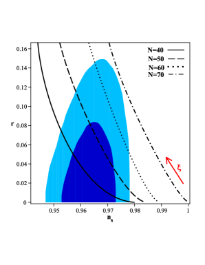
Figure 1: Evolution of the tensor to scalar ratio (left panel) and running of the scalar spectral index (right panel) versus the scalar spectral index, for a non-minimally coupled DGP model with a quadratic potential, in the background of Planck+WMAP9+BAO data. The figure has been plotted for four values of the number of e-folds. The non-minimal coupling parameter, $\xi$, increases in the direction of the red arrow. For $N=70$, the non-minimally coupled DGP setup is well outside the $95\%$ CL of the Planck+WMAP9+BAO data for all values of $\xi$. For other values of $N$, the model lies inside the $95\%$ CL of the Planck+WMAP9+BAO data for some values of $\xi$.

3.2 $V(\varphi)=\frac{\sigma}{4}\varphi^{4}$

The next potential we consider, is a quartic potential. It has been confirmed with WMAP9 [31] and Planck [26] data that, a model with a quartic potentia in 4-dimension lies outside the $95\%$ CL. In our branworld setup we reach a different result: a minimally coupled DGP model with this potential, lies inside the $95\%$ CL of WMAP7+BAO+H₀ data for $30\leq N\leq 60$, and lies inside the $95\%$ CL of the Planck+ WMAP9+ BAO data for $30\leq N\leq 46$. If we consider a non-minimally coupled scalar field on the DGP brane, the model lies inside the $95\%$ CL of the Planck+WMAP9+BAO data for $N>46$ too. We have studied the behavior of the inflationary parameters in the non-minimally coupled DGP model for $N=40,\,50,\,60\,$ and 70 and for $\xi\geq 0$ in the background of Planck+WMAP9+BAO data. The result is shown in figure 2. For $N=70$, with all values of $\xi$, the model is well outside the $95\%$ CL of the Planck+WMAP9+BAO data. For $N=60$, the model with $0.09\leq\xi\leq 0.108$ lies inside the $95\%$ CL of the data. For $N=50$, the model with $0.51\leq\xi\leq 0.0891$ and $0.11<\xi\leq 0.131$ is compatible with the Planck+WMAP9+BAO data. For $N=40$, the model with $\xi\leq 0.101$ and $\xi\geq 0.1308$ is well inside the the $95\%$ CL of the Planck+WMAP9+BAO data. Note that the evolution of the running of the scalar spectral index corresponding to the quartic potential is shown in the right panel of figure 2. The value of the running of the spectral index is negative and very close to zero for all values of $\xi$.

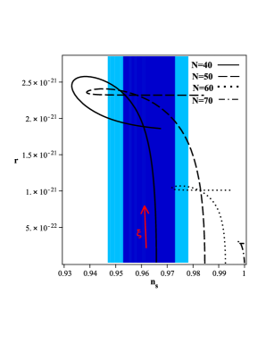
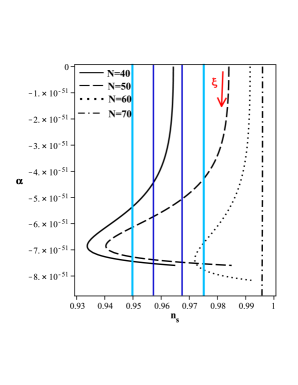
Figure 2: Evolution of the tensor to scalar ratio (left panel) and running of the scalar spectral index (right panel) versus the scalar spectral index, for a non-minimally coupled DGP model with a quartic potential, in the background of Planck+WMAP9+BAO data. The figure has been plotted for $N=40,\,50,\,60\,$ and $70$ and with $\xi\geq 0$. For $N=70$, the non-minimally coupled DGP setup is well outside the $95\%$ CL of the Planck+WMAP9+BAO data for all values of $\xi$. For other values of $N$, the model lies inside the $95\%$ CL of the Planck+WMAP9+BAO data in some range of $\xi$.

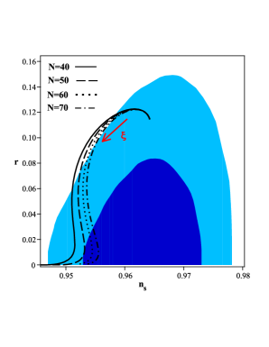
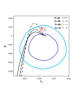
Figure 3: Evolution of the tensor to scalar ratio (left panel) and running of the scalar spectral index (right panel) versus the scalar spectral index, for a non-minimally coupled DGP model with a linear potential, in the background of Planck+WMAP9+BAO data. The figure has been plotted for $N=40,\,50,\,60\,$ and $70$ and with $\xi\geq 0$. For all given values of the number of e-folds, the non-minimally coupled DGP setup in some range of $\xi$ lies inside the $95\%$ CL of the Planck+WMAP9+BAO.

3.3 $V(\varphi)=\sigma\varphi$

Now, we consider a linear inflationary potential as $V=\sigma\varphi$ [32] which is motivated by axion monodromy. A minimally coupled four-dimensional setup with this potential lies within the $95\%$ CL of the Planck+WMAP9+BAO data [26]. Our braneworld model (either minimally or non-minimally coupled setup), with this linear potential, lies within the $95\%$ CL of WMAP7+BAO+H₀. A minimally coupled DGP model with this potential lies still inside the $95\%$ CL of the Planck+WMAP9+BAO data. But, there are constraints on the parameters in the non-minimal coupling case. As other cases, we consider four values of number of e-folds. In the left panel of figure 3, we see the evolution of the tensor to scalar ratio versus the scalar spectral index with $\xi\geq 0$. Our numerical analysis shows that, a DGP model with a non-minimally coupled scalar field, in some range of $\xi$ is observationally viable. For $N=70$, the model with $\xi\leq 0.021$ and $0.3201\leq\xi$ lies inside the $95\%$ CL of the Planck+WMAP9+BAO data. For $N=60$, the model with $\xi\leq 0.0195$ and $0.0383\leq\xi$ is compatible with data. For $N=50$, the non-minimally coupled DGP model with $\xi\leq 0.0193$ and $0.0461\leq\xi$ is within the $95\%$ CL of the Planck+WMAP9+BAO data. Finally, for $N=40$, the model with $\xi<0.0192$ and $0.0602<\xi<0.1301$ lies within the range of observational data. The right panel of figure 3 shows the evolution of the running of the scalar spectral index versus the scalar spectral index. As the figure shows, for a non-minimally coupled DGP model with a linear potential, the running of the scalar spectral index is negative. The value of running in this case is relatively large.

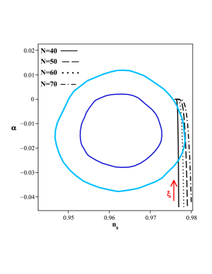
Figure 4: Evolution of the tensor to scalar ratio (left panel) and running of the scalar spectral index (right panel) versus the scalar spectral index, for a non-minimally coupled DGP model with a potential of type $V(\varphi)\sim\varphi^{\frac{2}{3}}$, in the background of Planck+WMAP9+BAO data. The figure has been plotted for $N=40,\,50,\,60\,$ and $70$ and with $\xi\geq 0$. For all given values of the number of e-folds, the non-minimally coupled DGP setup in some range of $\xi$ lies inside the $95\%$ CL of the Planck+WMAP9+BAO data.

3.4 $V(\varphi)=\sigma\varphi^{\frac{2}{3}}$

In this subsection we adopt another type of potential motivated by axion monodromy, as $V(\varphi)=\sigma\varphi^{\frac{2}{3}}$ [33]. As shown in Ref. [26], a minimally coupled 4-dimensional model with this type of potential lies within the $95\%$ CL of the Planck+WMAP9+BAO data. Although a minimally coupled DGP model with this potential lies in the $95\%$ CL of the WMAP7+BAO+H₀, it is now well outside the $95\%$ CL of the Planck+WMAP9+BAO data. If we consider a non-minimally coupled scalar field on the DGP brane, we find that the model in some range of $\xi$ is compatible with newly released observational data. The evolution of the tensor to scalar ratio versus the scalar spectral index is shown in the left panel of figure 4. For $N=70$, the non-minimally coupled DGP model with $\xi\geq 0.076$, for $N=60$, the model with $\xi\geq 0.0768$, for $N=50$, the model with $\xi\geq 0.0775$ and for $N=40$, the model with $\xi\geq 0.078$ lies inside the $95\%$ CL of the Planck+WMAP9+BAO data. Note that, as $\xi$ increases the non-minimally coupled DGP model with this potential becomes independent of the value of $N$. We have also plotted the evolution of the running of the scalar spectral index versus the scalar spectral index (right panel of figure 4). For this case, the running is negative and in some range of $\xi$ is compatible with recent data.

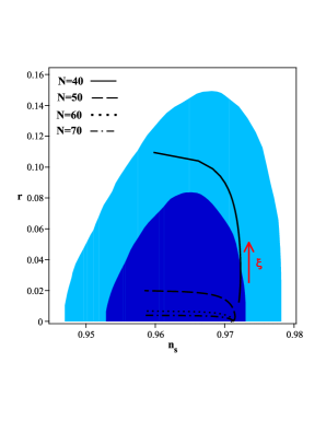
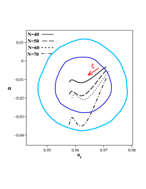
Figure 5: Evolution of the tensor to scalar ratio (left panel) and running of the scalar spectral index (right panel) versus the scalar spectral index, for a non-minimally coupled DGP model with an exponential potential of the type $V(\varphi)\sim\exp(-\beta\varphi)$, in the background of the Planck+WMAP9+BAO data. The figure has been plotted for $N=40,\,50,\,60\,$ and $70$ and with $\xi\geq 0$. For all given values of the number of e-folds, the non-minimally coupled DGP setup with all values of $\xi$ lies inside the $95\%$ CL of the Planck+WMAP9+BAO data.

3.5 $V(\varphi)=V_{0}\exp(-\beta\varphi)$

Here, we study the inflationary parameter with an exponential potential where $\beta$ is a positive constant. With this type of potential, a 4-dimensional model is well outside the $95\%$ CL (even, $0.99.7\%$ CL) of the Planck+WMAP9+BAO data (see [26]). For a DGP model with this potential and with either minimally or non-minimally coupled scalar field on the brane, we reach different results. This model with an exponential potential with all values of $\xi$ lies inside the $95\%$ CL of the Planck+WMAP9+BAO data. In the left panel of figure 5, we see the evolution of the tensor to scalar ratio versus the scalar spectral index in the background of the Planck+WMAP9+BAO data. As we see the models with number of e-folds $N=50,\,60,\,70$ give more reasonable results than the $N=40$ case. The right panel of figure 5 shows the behavior of the running of the spectral index versus the spectral index. With an exponential potential, the running is large and negative.

3.6 $V(\varphi)=V_{0}\exp(\beta\varphi)$

In this subsection we consider another type of exponential potential with positive exponent. A minimally coupled DGP model with this potential lies outside the the $95\%$ CL of the WMAP7+BAO+H₀ data and even $95\%$ CL of the Planck+WMAP9+BAO data. However, a non-minimally coupled DGP model with this exponential potential, in some range of $\xi$, is compatible with observational data. The left panel of the figure 6 shows the behavior of the tensor to scalar ratio versus the scalar spectral index with $\xi\geq 0$. For, $N=70$, the non-minimally coupled DGP model with $0.0431\leq\xi\leq 0.1301$, for $N=60$, the model with $0.0442<\xi\leq 0.127$, for $N=50$, the model with $0.052\leq\xi\leq 0.101$ and for $N=40$, the model with $0.058\leq\xi\leq 0.0621$ lies inside the $95\%$ CL of the Planck+WMAP9+BAO data. The left panel of the figure 6 shows the evolution of the running of the spectral index versus the scalar spectral index. With this exponential potential, the running is negative in some range of $\xi$ and is positive in other ranges. For $N=70$ the running of the spectral index with $\xi\geq 0.046$, for $N=60$ the running with $\xi\geq 0.04201$, for $N=50$ the running with $\xi\geq 0.0372$ and for $N=40$ the running with $\xi\geq 0.0291$ is negative.

In table 1, we have summarized the result of our numerical analysis in a non-minimally coupled DGP model. We have clearly specified the range of the non-minimal coupling parameter in which the model is compatible with Planck+WMAP9+BAO data.

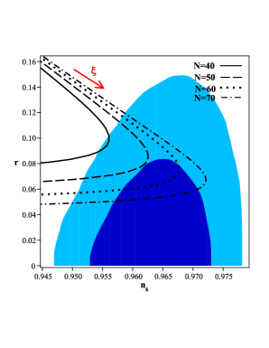
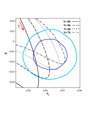
Figure 6: Evolution of the tensor to scalar ratio (left panel) and running of the scalar spectral index (right panel) versus the scalar spectral index, for a non-minimally coupled DGP model with an exponential potential of the type $V(\varphi)\sim\exp(\beta\varphi)$, in the background of the Planck+WMAP9+BAO data. The figure has been plotted for $N=40,\,50,\,60\,$ and $70$ and with $\xi\geq 0$. For all given values of the number of e-folds, the non-minimally coupled DGP setup in some range of $\xi$ lies inside the $95\%$ CL of the Planck+WMAP9+BAO data. Also, the running of the scalar spectral index is negative just in some ranges of $\xi$.

Table 1: The range of $\xi$ for which a non-minimally coupled DGP model lies inside the Planck+WMAP9+BAO data.

$V$	$N=40$	$N=50$	$N=60$	$N=70$
$\frac{\sigma}{2}\varphi^{2}$	$0.011<\xi<0.0553$	$0.032\leq\xi\leq 0.0784$	$0.051\leq\xi<0.09$	—
$\frac{\sigma}{4}\varphi^{4}$	$\xi\leq 0.101$	$0.51\leq\xi\leq 0.0891$	$0.09\leq\xi\leq 0.108$	—
	and $\xi\geq 0.1308$	and $0.11<\xi\leq 0.131$
$\sigma\varphi$	$\xi<0.0192$	$\xi\leq 0.0193$	$\xi\leq 0.0195$	$\xi\leq 0.021$
	and $0.0602<\xi<0.1301$	and $0.0461\leq\xi$	and $0.0383\leq\xi$	and $0.3201\leq\xi$
$\sigma\varphi^{\frac{2}{3}}$	$0.078\leq\xi$	$0.078\leq\xi$	$0.0768\leq\xi$	$0.076\leq\xi$
$V_{0}e^{-\beta\varphi}$	all values of $\xi$	all values of $\xi$	all values of $\xi$	all values of $\xi$
$V_{0}e^{\beta\varphi}$	$0.058\leq\xi\leq 0.0621$	$0.052\leq\xi\leq 0.101$	$0.0442<\xi\leq 0.127$	$0.0431\leq\xi\leq 0.1301$

4 Conclusion

In this paper we have studied the observational status of a non-minimal inflation model on a warped DGP braneworld scenario. By choosing some well-motivated types of potential, we have studied the evolution of the inflationary parameters in the background of the newly released Planck+WMAP9+BAO data. We have also, compared our result with those results obtained in a 4-dimensional setup and we found that the presence of the non-minimal coupling and the extra dimension causes considerable differences relative to the four dimensional case. Although a minimal 4D model with a quadratic potential lies inside the $95\%$ CL of the Planck+WMAP9+BAO data, a minimal DGP model with this potential is outside the data range. But, if we include an explicit non-minimal coupling between the scalar field and induced gravity on the brane, we find that the model with specific values of $N$ and in some ranges of the non-minimal coupling parameter lies well in the $95\%$ CL of the Planck+WMAP9+BAO data. With a quartic potential, the 4-dimensional model is well outside the $95\%$ CL of the Plank+WMAP9+BAO data whereas, the DGP model with specific values of $N$ lies within the $95\%$ CL of the Planck+WMAP9+BAO data. A non-minimally coupled DGP model in larger range of $N$ is compatible with Planck data. Both minimal 4D model and minimal DGP model, with a linear potential, lie inside the Planck data. But, a non-minimal DGP model with a linear potential is outside the $95\%$ CL of the Planck+WMAP9+BAO data, in some range of $\xi$. A minimal four dimensional model with potential of the type $V\sim\varphi^{\frac{2}{3}}$ lies inside the $95\%$ CL of the Planck+WMAP9+BAO data whereas, a minimal DGP model with this type of potential is outside the range of these observational data. In the presence of the non-minimal coupling, the DGP model in some range of $\xi$ lies inside the $95\%$ CL of the Planck+WMAP9+BAO data. It seems that, an exponential potential ($V\sim\exp(-\beta\varphi)$) is the best potential for a DGP model in an inflationary stage. With this potential, both minimally and non-minimally coupled DGP setup lie well inside the the $95\%$ CL of the Planck+WMAP9+BAO data. Note that, a four-dimensional model with this potential is quite outside the Planck data [26]. The last potential which we have considered in this paper is an exponential potential as $V\sim\exp(\beta\varphi)$. With this potential, a minimal DGP model lies outside the Planck data and a non-minimal DGP model, in some range of $\xi$ lies inside the $95\%$ CL of the Planck+WMAP9+BAO data. In summary, within a braneworld setup with induced gravity and a non-minimally coupled scalar field on the brane, a inflation model with $V\sim\exp(-\beta\varphi)$ has the best fit with the recent observational data.

References

• [1] A. Guth, Phys. Rev. D, 62, 105030, (1981).
• [2] A. D. Linde, Phys. Lett. B, 108, 389 (1982)
• [3] A. Albrecht and P. Steinhard, Phys. Rev. D, 48, 1220, (1982)
• [4] A. D. Linde, Particle Physics and Inflationary Cosmology (Harwood Academic Publishers, Chur, Switzerland, 1990).
• [5] A. Liddle and D. Lyth, Cosmological Inflation and Large-Scale Structure, (Cambridge University Press, 2000).
• [6] J. E. Lidsey et al, Phys. Rev. D, 69, 373, (1997).
• [7] A. Riotto, [arXiv:hep-ph/0210162].
• [8] D. H. Lyth and A. R. Liddle, The Primordial Density Perturbation (Cambridge University Press, 2009).
• [9] R. H. Brandenberger, [arXiv:hep-th/0509099].
• [10] R. Maartens, D. Wands, B. Bassett, I. Heard, Phys. Rev. D, 62, 041301, (2000).
• [11] R. Cai and H. Zhang, JCAP, 0408, 017, (2004)
• [12] S. del Campo and R. Herrera, Phys. Lett. B, 653, 122, (2007).
• [13] K. Nozari, M. Shoukrani and B. Fazlpour, Gen. Rel. Grav, 43, 207, (2011).
• [14] K. Nozari and N. Rashidi, Phys. Rev. D, 86, 043505, (2012).
• [15] V. Faraoni, Phys. Rev. D, 53, 6813, (1996).
• [16] V. Faraoni, Phys. Rev. D, 62, 023504, (2000).
• [17] V. Faraoni, Int. J. Theor. Phys., 38, 217, (1999).
• [18] R. Fakir, S. Habib and W. G. Unruh, Astrophys. J., 394, 396, (1992).
• [19] M. V. Libanov, V. A. Rubakov and P. G. Tinyakov, Phys. Lett. B, 442, 63, (1998).
• [20] J. Hwang and H. Noh, Phys. Rev. D, 60, 123001, (1999).
• [21] S. Tsujikawa, K. Maeda and T. Torii, Phys. Rev. D, 60, 063515, (1999a).
• [22] K. Nozari and S. Shafizadeh, Phys. Scr. 82, 015901, (2010).
• [23] S. Nojiri, S. D. Odintsov [arXiv:0807.0685].
• [24] G. Cognola, E. Elizalde, S. Nojiri, S.D. Odintsov, L. Sebastiani and S. Zerbini, Phys. Rev. D 77, 046009, (2008).
• [25] S. Nojiri, S. D. Odintsov, Phys. Rev. D, 77, 026007, (2008).
• [26] P. A. R. Ade et al., [arXiv:1303.5082].
• [27] J. Bardeen, Phys. Rev. D, 22, 1882, (1980).
• [28] V. F. Mukhanov, H. A. Feldman and R. H. Brandenberger, Phys. Rept., 215, 203, (1992).
• [29] E. Bertschinger, [arXiv:astro-ph/9503125].
• [30] E. Komatsu et al., Astrophys. J. Suppl., 192, 18, (2011).
• [31] Hinshaw et al., [arXiv:1212.5226], (2013).
• [32] L. McAllister, E. Silverstein and A. Westphal, Phys. Rev., D 82, 046003, (2010).
• [33] E. Silverstein and A. Westphal, Phys. Rev., D 78, 106003, (2008)