Comprehending heavy charmonia and their decays by hadron loop effects

Abstract

We present that including the hadron loop effects could help us to understand the spectrum of the heavier charmonium-like states and their decays simultaneously. The observed states could be represented by the poles on the complex energy plane. By coupling to the opened thresholds, the pole positions are shifted from the bare states predicted in the quenched potential model to the complex plane. The pole masses are generally pulled down from the bare masses and the open-charm decay widths are related to the imaginary parts of the pole positions. Moreover, we also analyze the pole trajectory of the $\chi_{c1}(2P)$ state while the quark pair production rate from the vacuum changes in its uncertainty region, which indicates that the enigmatic $X(3872)$ state may be regarded as a $1^{++}$ $c\bar{c}$ charmonium-dominated state dressed by the hadron loops as the others.

I Introduction

Before the $X(3872)$ was found Choi et al. (2003), there were only four well-established charmonium states above the $D\bar{D}$ threshold. In recent years, along with explosion of the experimental activities on the heavy quarkonium physics, more than a dozen of charmonium-like $``XYZ"$ states above the open-flavor thresholds have been observed and the charmonium family is remarkably enriched. Until now, there are fourteen neutral charmonium-like states quoted in the Particle Data Group (PDG) Table Beringer et al. (2012). However, the masses of most newly observed states above open-charm thresholds run out of the predictions of the quark potential model Godfrey and Isgur (1985) which proved to be successful for those states below the $D\bar{D}$ threshold. Therefore, different approaches are adopted to understand them case by case and there is no consensus on the natures of those “unexpected” states.

$X(3872)$ is a typical example in this situation. Its mass is too low to be a $2P$ $c\bar{c}$ state in the potential model Barnes and Godfrey (2004) and this possibility was almost given up, after the isospin violating decay $X\rightarrow J/\psi\rho$ was confirmed. As the state is located just at the $D\bar{D}^{*}$ threshold, it is also suggested to be a $D\bar{D}^{*}$ molecule bounded by pion exchanges Tornqvist (2004); Close and Page (2004); Voloshin (2004); Wong (2004); Braaten and Kusunoki (2004). This assignment can explain the properties of the mass and the $J^{PC}$ of $X(3872)$, but it encounters serious problems in other aspects. For example, as a loosely bounded $D\bar{D}^{*}$ molecule, it is difficult to radiatively transit into excited charmonium states, such as $\psi^{\prime}$, through the quark annihilation or other mechanisms. The BaBar collaboration Aubert et al. (2009) measured the ratio ${Br(X\rightarrow\psi^{\prime}\gamma)/Br(X\rightarrow\psi\gamma)}=3.4\pm 1.4,$ which is several orders of magnitude higher than the model predictions, e.g. in Ref. Swanson (2004a, b).

The difficulties also remind theorists that the vacuum fluctuation effect should receive more attention in understanding the heavier charmonia. In the quark potential models, a charmonium state is considered as a bound state of a charm quark and its antiquark through a non-relativistic interaction potential, typically incorporating a Coulomb term at a short distance and a linear confining term at a large distance. These models neglect the modifications due to quantum fluctuations, i.e., the creation of light quark pairs, which can be represented by the hadron loops in the coupled channel model. This coupled channel effect was considered in the Cornell model, Eichten et al. (1978) and it has also been used to study the resonances with strongly coupled S-wave thresholds, where the states are drawn to their strongly coupled thresholds van Beveren et al. (1983). In particular, Heikkil$\ddot{\mathrm{a}}$, T$\ddot{\mathrm{o}}$rnqvist, and Ono developed a unitarized quark model, carrying over the Dyson summation idea, to study the charmonium spectrum long ago Heikkila et al. (1984). Recently, Pennington and Wilson Pennington and Wilson (2007) extracted the mass shifts of charmonium states from the results of a non-relativistic potential model by Barnes, Godfrey, and Swanson Barnes et al. (2005) by considering the hadron loop effect. K.T.Chao and his collaborators also proposed a screened potential model Chao and Liu (1989); Li and Chao (2009) to investigate the heavy quarkonium spectrum, in which the effect of vacuum polarization is incorporated in a different way.

Our present study goes along the same lines as Ref. Pennington and Wilson (2007) with several significant improvements. First, instead of using an empirical universal form factor to describe the coupling vertices between the charmonium states and the decaying channels as in Pennington and Wilson (2007), we formulate the vertex functions by adopting the ${}^{3}P_{0}$ model so that they could be represented by the parameters in the potential model. Secondly, incorporating the ${}^{3}P_{0}$ model into this scheme also enables us to produce not only the mass shifts but also the decay widths, whereas the decay widths are inputs in Ref. Pennington and Wilson (2007) extracted from Ref. Barnes et al. (2005). Moreover, this analytical formulation also shows more merits by allowing us to explore the poles on the complex energy plane, whose behaviors as the parameters change shed more insight on the nature of these states, especially with regard to the enigmatic $X(3872)$ state. It is also worth mentioning that this calculation covers all the related charmonium states in one unified picture instead of treating them case by case.

In this study, we found that the discrepancies between the observed masses and the predictions of the quenched potential model could be compensated by taking the hadron loop effect into account. Meanwhile, their open-charm decay widths are reproduced in a reasonable manner. That means, most of the states discussed in this paper could be depicted in a unified picture, as a charmonium state dressed by hadron loops, or similarly, as a mixture of a conventional charmonium state and the coupled continuums. The enigmatic $X(3872)$ could also be included in this scheme without any “exotic” aspect.

The paper is organized as follows: In Section II, the main scheme and how to model the coupled channels are briefly introduced. Numerical procedures and results are discussed in Section III. Section IV is devoted to our conclusions and further discussions.

II The model

In a non-relativistic quark potential model, a quarkonium meson is regarded as a bound state of a quark and an anti-quark, formed by the effective potential generated from the gluon exchange diagrams and, in certain circumstances, the annihilation diagrams. At the hadron level, the bare propagator of such a bound state could be represented as

$$\mathbb{P}(s)=1/(m_{0}^{2}-s),$$ (1)

with a pole on the real axis of the complex $s$ plane, corresponding to a non-decaying state, where $m_{0}$ is the mass of the “bare” $q\bar{q}$ state. Once its coupling to certain two-body channels is considered, the inverse meson propagator, $\mathbb{P}^{-1}(s)$, is expressed as

$$\mathbb{P}^{-1}(s)=m_{0}^{2}-s+\Pi(s)=m_{0}^{2}-s+\sum_{n}\Pi_{n}(s),$$ (2)

and $\Pi_{n}(s)$ is the self-energy function for the $n$-th coupling channel. Here, the sum is over all the opened channels and, in principle, all virtual channels. $\Pi_{n}(s)$ is an analytic function with only a right-hand cut starting from the $n$-th threshold $s_{th,n}$, and so, one can write down its real part from its imaginary part through a dispersion relation

$$\mathrm{Re}\Pi_{n}(s)=\frac{1}{\pi}\mathcal{P}\int_{s_{th,n}}^{\infty}\mathrm{d}z\frac{\mathrm{Im}\Pi_{n}(z)}{(z-s)},$$ (3)

where $\mathcal{P}\int$ means the principal value integration. The mass and total width of a meson are specified by a pole of $\mathbb{P}(s)$ on the unphysical Riemann sheet attached to the physical region, usually defined as $s_{pole}=(M_{pole}-i\Gamma_{pole}/2)^{2}$. This mechanism is typified by the Dyson-Schwinger equation for the propagator of the $\rho$ meson as illustrated in Ref.Pennington (2010). As the bare $\rho$ state predominantly couples to the $\pi\pi$ system in the $P$ wave, the pole will move away from the real axis onto the complex energy plane, thus the $\rho$ meson could be regarded as largely a $q\bar{q}$ state with a few percent $\pi\pi$. Geiger and Isgur (1993)

To investigate the pole positions in this scheme, we make use of the Quark Pair Creation (QPC) model Micu (1969); Colglazier and Rosner (1971); Le Yaouanc et al. (1973), also known as the ${}^{3}P_{0}$ model in the literature, to model the coupling vertices of the imaginary part of the self-energy function in this calculation. This is not only because this model has proved to be successful in many phenomenological calculations but also because it could provide analytical expressions of the vertex functions. Furthermore, the exponential factors in the vertex functions of the QPC model provide a natural ultraviolet suppression to the dispersion relation, which is chosen by hand according to the empirical strong interaction length scale in Ref. Pennington and Wilson (2007).

A modern review of the QPC model and calculation of the transition amplitude can be found in Ref.Luo et al. (2009). The main ingredients of this model are summarized in the following. In the QPC model, a meson (with a quark $q_{1}$ and an anti-quark $q_{2}$) decay occurs by producing a quark ($q_{3}$) and anti-quark ($q_{4}$) pair from the vacuum. In the non-relativistic limit, the transition operator is represented as

$$T=-3\gamma\sum_{m}\langle 1m1-m|00\rangle\int d^{3}\vec{p_{3}}d^{3}\vec{p_{4}}\delta^{3}(\vec{p_{3}}+\vec{p_{4}})$$

$$\mathcal{Y}_{1}^{m}(\frac{\vec{p_{3}}-\vec{p_{4}}}{2})\chi_{1-m}^{34}\phi_{0}^{34}\omega_{0}^{34}b_{3}^{\dagger}(\vec{p_{3}})d_{4}^{\dagger}(\vec{p_{4}}),$$ (4)

where $\gamma$ is a dimensionless parameter to represent the quark pair production rate from the vacuum, and $\mathcal{Y}_{1}^{m}(\vec{p})\equiv p^{l}Y_{l}^{m}(\theta_{p},\phi_{p})$ is a solid harmonic function that gives the momentum-space distribution of the created pair. Here the spins and relative orbital angular momentum of the created quark and anti-quark (referred to by subscripts $3$ and $4$, respectively) are combined to give the overall $J^{PC}=0^{++}$ quantum numbers. $\phi_{0}^{34}=(u\bar{u}+d\bar{d}+s\bar{s})/\sqrt{3}$ and $\omega_{0}^{34}=\delta_{ij}$, where $i$ and $j$ are the SU(3)-color indices of the created quark and anti-quark. $\chi_{1-m}^{34}$ is a triplet of spin. The helicity amplitude $\mathcal{M}^{M_{J_{A}},M_{J_{B}},M_{J_{C}}}$ is from the transition amplitude

$$\langle BC|T|A\rangle=\delta^{3}(K_{B}+K_{C}-K_{A})\mathcal{M}^{M_{J_{A}},M_{J_{B}},M_{J_{C}}}.$$ (5)

(see Ref.Luo et al. (2009) for the details).

Thus, the imaginary part of the self-energy function in the dispersion relation, Eq.(3), could be expressed as

$$Im\Pi_{A\rightarrow BC}(s)=-\frac{\pi^{2}}{2J_{A}+1}\frac{|\vec{P}(s)|}{\sqrt{s}}$$

$$\sum_{M_{J_{A}},M_{J_{B}},M_{J_{C}}}|\mathcal{M}^{M_{J_{A}},M_{J_{B}},M_{J_{C}}}(s)|^{2},$$ (6)

where $|P(s)|$ is the three-momentum of $B$ and $C$ in their center of mass frame. So,

$$\frac{|P(s)|}{\sqrt{s}}=\frac{\sqrt{(s-(m_{B}+m_{C})^{2})(s-(m_{B}-m_{C})^{2})}}{2s}.$$ (7)

The $A-BC$ amplitude reads

$$\mathcal{M}^{M_{J_{A}}M_{J_{B}}M_{J_{C}}}(\vec{P}) = \gamma\sqrt{8E_{A}E_{B}E_{C}}\sum_{M_{L_{A}},M_{S_{A}},M_{L_{B}},M_{S_{B}},M_{L_{C}},M_{S_{C}},m}\langle L_{A}M_{L_{A}}S_{A}M_{S_{A}}|J_{A}M_{J_{A}}\rangle$$ (8)

$$\times\langle L_{B}M_{L_{B}}S_{B}M_{S_{B}}|J_{B}M_{J_{B}}\rangle\langle L_{C}M_{L_{C}}S_{C}M_{S_{C}}|J_{C}M_{J_{C}}\rangle\langle 1m1-m|00\rangle$$

$$\times\langle\chi_{S_{C}M_{S_{C}}}^{32}\chi_{S_{B}M_{S_{B}}}^{14}|\chi_{S_{A}M_{S_{A}}}^{12}\chi_{1-m}^{34}\rangle\langle\phi_{C}^{32}\phi_{B}^{14}|\phi_{A}^{12}\phi_{0}^{34}\rangle I_{M_{L_{B}},M_{L_{C}}}^{M_{L_{A}},m}(\vec{P}).$$

The spatial integral $I_{M_{L_{B}},M_{L_{C}}}^{M_{L_{A}},m}(\vec{P})$ is given by

$$I_{M_{L_{B}},M_{L_{C}}}^{M_{L_{A}},m}(\vec{P})=\int d^{3}\vec{k}\psi^{*}_{n_{B}L_{B}M_{L_{B}}}(-\vec{k}+\frac{\mu_{4}}{\mu_{1}+\mu_{4}}\vec{P})$$

$$\times\psi^{*}_{n_{C}L_{C}M_{L_{C}}}(\vec{k}-\frac{\mu_{3}}{\mu_{2}+\mu_{3}}\vec{P})\psi_{n_{A}L_{A}M_{L_{A}}}(-\vec{k}+\vec{P})\mathcal{Y}_{1}^{m}(\vec{k}),$$

where we have taken $\vec{P}\equiv\vec{P_{B}}=-\vec{P_{C}}$ and $\mu_{i}$ is the mass of the $i$-th quark. $\psi_{n_{A}L_{A}M_{L_{A}}}(\vec{k_{A}})$ is the relative wave function of the quarks in meson $A$ in the momentum space.

The recoupling of the spin matrix element can be written, in terms of the Wigner’s $9$-$j$ symbol, as

$$\langle\chi_{S_{C}M_{S_{C}}}^{32}\chi_{S_{B}M_{S_{B}}}^{14}|\chi_{S_{A}M_{S_{A}}}^{12}\chi_{1-m}^{34}\rangle$$

$$=[3(2S_{B}+1)(2S_{C}+1)(2S_{A}+1)]^{1/2}$$

$$\times\sum_{S,M_{S}}\langle S_{C}M_{S_{C}}S_{B}M_{S_{B}}|SM_{S}\rangle\langle SM_{S}|S_{A}M_{S_{A}};1,-m\rangle$$

$$\times\left\{\begin{array}[]{ccc}1/2&1/2&S_{C}\\ 1/2&1/2&S_{B}\\ S_{A}&1&S\\ \end{array}\right\}.$$ (13)

The flavor matrix element is

$$\langle\phi_{C}^{32}\phi_{B}^{14}|\phi_{A}^{12}\phi_{0}^{34}\rangle$$

$$=\sum_{I,I^{3}}\langle I_{C},I_{C}^{3};I_{B}I_{B}^{3}|I_{A}I_{A}^{3}\rangle$$

$$\times[(2I_{B}+1)(2I_{C}+1)(2I_{A}+1)]^{1/2}\left\{\begin{array}[]{ccc}I_{2}&I_{3}&I_{C}\\ I_{1}&I_{4}&I_{B}\\ I_{A}&0&I_{A}\\ \end{array}\right\},$$ (17)

where $I_{i}(I_{1},I_{2},I_{3},I_{4})$ is the isospin of the quark $q_{i}$.

With all the necessary ingredients of the model at hand, care must be taken when Eq.(II) is continued to the complex $s$ plane for extracting the related poles. Since what is used in this model is only the tree level amplitude, there is no right hand cut for the amplitude, $\mathcal{M}^{M_{J_{A}},M_{J_{B}},M_{J_{C}}}(s)$. Thus, the analytical continuation of the amplitude obeys $\mathcal{M}(s+i\epsilon)^{*}=\mathcal{M}(s-i\epsilon)=\mathcal{M}(s+i\epsilon)$. The physical amplitude, incorporating the loop contributions, should have right hand cuts, and, in principle, the analytical continuation turns to be $\mathcal{M}(s+i\epsilon)^{*}=\mathcal{M}(s-i\epsilon)=\mathcal{M}^{II}(s+i\epsilon)$ by meeting the need of real analyticity. $\mathcal{M}^{II}(s+i\epsilon)$ means the amplitude on the unphysical Riemann sheet attached with the physical region.

The general character of the poles on different Riemann sheets has been discussed widely in the literature, (see, for example, Eden and Taylor (1964)). A resonance is represented by a pair of conjugate poles on the Riemann sheet, as required by the real analyticity. The micro-causality tells us the first Riemann sheet is free of complex-valued poles, and the resonances are represented by those poles on unphysical sheets. The resonance behavior is only significantly influenced by those nearby poles, and that is why only those closest poles to the experiment region could be extracted from the experiment data in a phenomenological study. Those poles on the other sheets, which are reached indirectly, make less contribution and are thus harder to determine.

III Numerical calculations and discussions

In this scheme, all the intermediate hadron loops will contribute to the “renormalization” of the “bare” mass of a bound state. It is easy to find that an opened channel will contribute both a real part and an imaginary part to the self-energy function, but a virtual channel contributes only a real one. To avoid counting the contributions of all virtual channels, we adopt a once-subtracted dispersion relation, as proposed in Ref. Pennington and Wilson (2007), to suppress contributions of the faraway “virtual” channels and to make the picture simpler. It is reasonable to expect that this lowest charmonium state, as a deep bound state, has the mass defined by the potential model, uninfluenced by the effect of the hadron loops. Its mass then essentially defines the mass scale and fixes the subtraction point. Thus, the subtraction point $s_{0}$ is chosen at the mass square of the $J/\psi$ state. The inverse of the meson propagator turns out to be

$$\mathbb{P}^{-1}(s)=m_{pot}^{2}-s+\sum_{n}\frac{s-s_{0}}{\pi}\int_{s_{th,n}}^{\infty}\mathrm{d}z\frac{\mathrm{Im}\Pi_{n}(z)}{(z-s_{0})(z-s)},$$

where $m_{pot}$ is the bare mass of a certain meson defined in the potential model.

The bare masses of the charmonium-like states in this calculation are chosen at the values of the classic work by Godfrey and Isgur (Refered to GI in the following) Godfrey and Isgur (1985). The reason why we choose this set of values is that they provide globally reasonable predictions to meson spectra with $u$, $d$, $s$, $c$, and $b$ quarks, especially those states below open-flavor thresholds. Thus, the constants used in our calculation of the coupling vertex is defined as the values in Ref. Godfrey and Isgur (1985) for consistency. The constituent quark masses are $M_{c}=1.628\mathrm{GeV}$, $M_{s}=0.419\mathrm{GeV}$, and $M_{u}=0.22\mathrm{GeV}$. The physical masses concerned in the final states are the average values in the PDG table. Beringer et al. (2012) We use the Simple Harmonic Oscillator (SHO) wave function to represent the relative wave function of quarks in a meson, as usually used in the QPC model calculation. The SHO wave function scale, denoted as the $\beta$ parameter, is from Ref.Godfrey and Kokoski (1991); Kokoski and Isgur (1987), which is chosen to reproduce the root mean square radius of the quark model state. For $D^{0}$, $D^{\pm}$, $D^{*0}$, $D^{*\pm}$, $D_{s}^{\pm}$, $D_{s}^{*\pm}$, the $\beta$ values are $0.66$, $0.66$, $0.54$, $0.54$, $0.71$, $0.59$, respectively, with units of $\mathrm{GeV}$. The $\beta$ parameters of the charmonium states of the GI’s model are reasonably estimated at a universal value of 0.4 $\mathrm{GeV}$, which is consistent with the average value in Ref. Close and Swanson (2005a). The dimensionless strength parameter is chosen at $\gamma=6.9$ for non-strange $q\bar{q}$ production, and $\gamma_{s}=\gamma/\sqrt{3}$ for $s\bar{s}$ production.Le Yaouanc et al.

It is also reasonable to assume that the parameters in the GI’s work have included part of the coupled channel effects, especially those virtual hadron loops, because part of the spectrum with open flavor thresholds have been covered in their fit. Furthermore, their predictions to those states below the $D\bar{D}$ threshold are quite precise, which also means the “renormalization” effects of those virtual hadron loops, which only contribute real parts in the dispersion relation, have entered the parameters. Thus, to avoid double counting, only those channels that could be open for a certain state are considered, as shown in Table 1.

In a general view, for the $3S$, $4S$, $2P$, $3P$, $1D$, and $2D$ states discussed in this paper, the pole masses are lower by about 10-110$\mathrm{MeV}$ than the predicted values in the quenched potential model, and the obtained pole masses agree better with the measured values. Moreover, even though the ${}^{3}P_{0}$ coupling is embedded in the scheme and the model parameters are fixed, the extracted pole widths are still reasonable compared with the experimental values for most of the states.

Table 1: The coupled channels of different states considered in this paper. The $D^{0}\bar{D}^{0}$ and $D^{+}\bar{D}^{-}$ modes are included in “$D\bar{D}$” and it is similar for “$D\bar{D}^{*}$” and “$D^{*}\bar{D}^{*}$”. The inclusion of the charge conjugate mode is always implied in this paper.

State ($n^{2S+1}L_{J}$)	$\ \ \ D\bar{D}\ \ \$	$\ \ \ D\bar{D}^{*}\ \ \$	$\ D^{*}\bar{D}^{*}\$	$\ \ \ D_{s}^{+}D_{s}^{-}$	$D_{s}^{+}D_{s}^{*-}$	$D_{s}^{*+}D_{s}^{*-}$
$\psi(3^{3}S_{1})$	$\Box$	$\Box$	$\Box$	$\Box$
$\eta_{c}(3^{1}S_{0})$		$\Box$
$\psi(4^{3}S_{1})$	$\Box$	$\Box$	$\Box$	$\Box$	$\Box$	$\Box$
$\eta_{c}(4^{1}S_{0})$		$\Box$	$\Box$		$\Box$	$\Box$
$\chi_{2}(2^{3}P_{2})$	$\Box$	$\Box$		$\Box$
$\chi_{1}(2^{3}P_{1})$		$\Box$
$\chi_{0}(2^{3}P_{0})$	$\Box$
$h_{c}(2^{1}P_{1})$		$\Box$
$\chi_{2}(3^{3}P_{2})$	$\Box$	$\Box$	$\Box$	$\Box$	$\Box$	$\Box$
$\chi_{1}(3^{3}P_{1})$		$\Box$	$\Box$		$\Box$	$\Box$
$\chi_{0}(3^{3}P_{0})$	$\Box$		$\Box$	$\Box$		$\Box$
$h_{c}(3^{1}P_{1})$		$\Box$	$\Box$		$\Box$	$\Box$
$\psi_{3}(1^{3}D_{3})$	$\Box$
$\psi(1^{3}D_{1})$	$\Box$
$\psi_{3}(2^{3}D_{3})$	$\Box$	$\Box$	$\Box$	$\Box$	$\Box$	$\Box$
$\psi_{2}(2^{3}D_{2})$		$\Box$	$\Box$		$\Box$	$\Box$
$\psi(2^{3}D_{1})$	$\Box$	$\Box$	$\Box$	$\Box$	$\Box$
$\eta_{c2}(2^{1}D_{2})$		$\Box$	$\Box$		$\Box$

Table 2: The compilation of the pole masses ($\mathrm{Re}[\sqrt{s_{pole}}]$) and the pole widths (2$\mathrm{Im}[\sqrt{s_{pole}}]$) of the states shifted by the hadron loops effects, compared to the observed values and the GI’s values. The unit is $\mathrm{MeV}$.

Multiplet	State ($n^{2S+1}L_{J}$)	$J^{PC}$	PDG State	Expt. mass	Expt. width	$\mathrm{Re}[\sqrt{s_{pole}}]$	2$\mathrm{Im}[\sqrt{s_{pole}}]$	GI mass
3S	$\psi(3^{3}S_{1})$	$1^{--}$	$\psi(4040)$	4039$\pm$1	80$\pm$10	4051	25	4100
	$\eta_{c}(3^{1}S_{0})$	$0^{-+}$				4025	23	4064
4S	$\psi(4^{3}S_{1})$	$1^{--}$	$X(4360)$	4361$\pm$13	74$\pm$18	4371	49	4450
	$\eta_{c}(4^{1}S_{0})$	$0^{-+}$				4348	48	4425
2P	$\chi_{2}(2^{3}P_{2})$	$2^{++}$	$\chi_{c2}^{\prime}$	3927$\pm$2	24$\pm$6	3942	2	3979
	$\chi_{1}(2^{3}P_{1})$	$1^{++}$	$X(3872)$	3872	$<$2.3	3884	4	3953
	$\chi_{0}(2^{3}P_{0})$	$0^{++}$	$X(3880)$?	3878$\pm$48?	347${}^{+316}_{-143}$?	3814	133	3916
	$h_{c}(2^{1}P_{1})$	$1^{+-}$	$X(3940)$	3942$\pm$9	37${}^{+27}_{-17}$	3900	6	3956
3P	$\chi_{2}(3^{3}P_{2})$	$2^{++}$				4244	24	4337
	$\chi_{1}(3^{3}P_{1})$	$1^{++}$				4217	84	4317
	$\chi_{0}(3^{3}P_{0})$	$0^{++}$	$X(4160)$	4160${}^{+29}_{-25}$	139${}^{+110}_{-60}$	4210	114	4292
	$h_{c}(3^{1}P_{1})$	$1^{+-}$				4219	49	4318
1D	$\psi_{3}(1^{3}D_{3})$	$3^{--}$				3838	1	3849
	$\psi_{2}(1^{3}D_{2})$	$2^{--}$						3838
	$\psi(1^{3}D_{1})$	$1^{--}$	$\psi(3770)$	3773	27$\pm$1	3764	18	3819
	$\eta_{c2}(1^{1}D_{2})$	$2^{-+}$						3837
2D	$\psi_{3}(2^{3}D_{3})$	$3^{--}$				4113	6	4217
	$\psi_{2}(2^{3}D_{2})$	$2^{--}$				4141	72	4208
	$\psi(2^{3}D_{1})$	$1^{--}$	$\psi(4160)$	4153$\pm$3	103$\pm$8	4080	114	4194
	$\eta_{c2}(2^{1}D_{2})$	$2^{-+}$				4101	44	4208

The potential model mass of the $\psi(1^{3}D_{1})$ state is at 3819 $\mathrm{MeV}$, while its pole is shifted down to $\sqrt{s}=$$(3.765-0.009i)$ $\mathrm{GeV}$ mass, which means that the pole mass is 3765 $\mathrm{MeV}$ and the pole width is 18 $\mathrm{MeV}$. These values are compatible with that of the observed $\psi(3770)$ state. The mass and width of $\psi(3770)$ are usually used to fit the model parameters, so this compatibility demonstrates the reasonability of the parameters we choose. Here, the $2S-1D$ mixing is not considered, since the mass of $\psi(2^{3}S_{1})$ predicted by the GI’s model is 3680 $\mathrm{MeV}$, which is below the $D^{0}\bar{D}^{0}$ threshold that it has no common opened channels with the $\psi(1^{3}D_{1})$. The mixing through their common virtual channels, which might leads to the large leptonic width of $X(3770)$ Rosner (2005), is beyond the scope of this study.

Since the masses of all the states are generally pulled down by considering the hadron loop effect and the spectrum is compressed, the $\psi(4415)$ seems to be too high to be assigned as the $\psi(4^{3}S_{1})$, although this assignment is held by the quenched potential model calculation Godfrey and Isgur (1985). The screened potential model Li and Chao (2009), which takes the vacuum fluctuation into account by introducing a screened potential, also suggests a compressed spectrum, in which the $\psi(4415)$ is proposed to have a $\psi(5^{3}S_{1})$ assignment. The pole properties of the $\psi(4^{3}S_{1})$ are more compatible with the $X(4360)$ state in this calculation.

In this paper, we did not find the space to accommodate the vector $X(4260)$ state, which is discovered by the BaBar Collaboration Aubert et al. (2005). Actually, there have already existed some difficulties to assign $X(4260)$ as a conventional charmonium in the liturature. The most serious one seems to be the observed dip rather than a peak in the $R$ value scanned in $e^{+}e^{-}$ annihilation Beringer et al. (2012) around $X(4260)$. Thus, this state could totally or partly be interpreted as an exotic state, such as a $c\bar{c}g$ hybrid Zhu (2005), a tetro-quark state Maiani et al. (2005); Ebert et al. (2008); Albuquerque and Nielsen (2009), a bayonium state Qiao (2008), or a molecule state Ding (2009). Another possibility for the dip is the destructive interference among the nearby resonances Chen et al. (2011).

The $X(3872)$ was first observed by Belle Choi et al. (2003) in the $J/\psi\pi^{+}\pi^{-}$ invariant mass distribution in $B^{+}\rightarrow K^{+}J/\psi\pi^{+}\pi^{-}$ decay as a very narrow peak around 3872 $\mathrm{MeV}$ with a width smaller than 2.3 $\mathrm{MeV}$. The CDF Collaboration update the mass of $X(3872)$ as

$$M(X(3872))=3871.61\pm 0.16\pm 0.19\mathrm{MeV},$$ (20)

which is just below the $D^{0}\bar{D}^{*0}$ threshold $m(D^{0}\bar{D}^{*0})=3871.81\pm 0.36\mathrm{MeV}$. Since this state is unexpected in the quenched potential model, its origin was widely discussed based on a molecule candidate of $D^{0}\bar{D}^{*0}$, a tetro-quark state, a charmonium state, or a charmonium state mixed with the $D^{0}\bar{D}^{*0}$ component (See Ref.Brambilla et al. (2011) and the references therein). Our calculation here supports the idea to regard $X(3872)$ as a charmonium state mixed with the $D^{0}\bar{D}^{*0}$ component, which is described in the language of hadron loops here. The bare mass of $\chi_{c1}(2^{3}P_{1})$ is at 3950 $\mathrm{MeV}$ in the GI’s model prediction, while its coupling to the $D^{0}\bar{D}^{*0}$ and $D^{+}\bar{D}^{*-}$ thresholds reduces its pole mass to 3884 $\mathrm{MeV}$ based on the parameter set we choose. The pole mass is just about 12 $\mathrm{MeV}$ higher than the observed mass of the $X(3872)$, and the related pole width is about 3 $\mathrm{MeV}$, which is comparable with the experimental data.

Moreover, it is worth pointing out that the $\gamma$ parameter of the QPC model usually has an uncertainty of about $30\%$ Close and Swanson (2005b), which is determined by fitting to the decay experiment data. The pole trajectory of $\chi_{c1}(2P)$ state is shown in Fig.1, with the $\gamma$ parameter ranging from $2.9$ to $8.9$. When this coupling is very weak, the pole of the $\chi_{c1}(2P)$ state is close to the bare state on the real energy axis, whose mass is $3950\mathrm{MeV}$ predicted in the GI’s model. Along with the strengthening of this coupling, the pole mass is pulled down with its width always below $10\mathrm{MeV}$. When the coupling become stronger at around $\gamma=7.6$, which is just $10\%$ away from the central value, the pole will reach the $D^{0}\bar{D}^{*0}$ threshold and then becomes a virtual bound state. Since the pole is shifted from the bare mass of $\chi_{c1}(2P)$, a charmonium origin of $X(3872)$ is easily suggested, or the $X(3872)$ could be regarded as a charmonium state dressed by the $D\bar{D}^{*}$ cloud. Such a mixed state is as compact as a conventional charmonium state, and this assignment could resolve the problems encountered by the molecule description in explaining the radiative transition $Br(X\rightarrow\psi^{\prime}\gamma)/Br(X\rightarrow\psi\gamma)$ ratio Aubert et al. (2009). This picture has some similarities with the other coupled channel analyses in Ref.Danilkin and Simonov (2010) and Ref. Coito et al. (2011), but we wish to point out that our calculation considers not only the $2P$ states but the charmonium-like spectrum systematically. Additionally, the authors of Zhang et al. (2009) used a coupled channel Flatt$\acute{\mathrm{e}}$ formula to fit the experimental data, and suggested that there may need to be two near-threshold poles to account for the data, one from the $D^{0}\bar{D}^{*0}$ component and the other from the charmonium state $\chi_{c1}(2P)$.

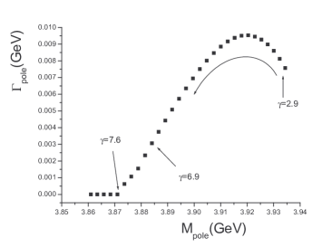
Figure 1: The trajectory of the pole parameters of the $\chi_{c1}(2P)$ state when the $\gamma$ parameter increases.

In the recoiling spectrum of $J/\psi$ in the $e^{+}e^{-}$ annihilation process $e^{+}e^{-}\rightarrow J/\psi+D\bar{D}^{*}$, the Belle group Abe et al. (2007); Pakhlov et al. (2008) found the evidence of the $X(3940)$, whose mass and width are determined as

$$M(X(3940)) = 3942^{+7}_{-6}\pm 6\mathrm{MeV},$$

$$\Gamma(X(3940)) = 37^{+26}_{-18}\pm 8\mathrm{MeV}.$$ (21)

Meanwhile, they also found the $X(4160)$ in the $D^{*}\bar{D}^{*}$ mode in the process $e^{+}e^{-}\rightarrow J/\psi+D^{*}\bar{D}^{*}$. The mass and width of $X(4160)$ are given by

$$M(X(4160)) = 4156^{+25}_{-20}\pm 15\mathrm{MeV},$$

$$\Gamma(X(4160)) = 139^{+111}_{-61}\pm 21\mathrm{MeV}.$$ (22)

Besides, there is a broad enhancement around $3880\mathrm{MeV}$ in the $D\bar{D}$ spectrum in $e^{+}e^{-}\rightarrow J/\psi+D\bar{D}$. Even though in Ref. Abe et al. (2007) the authors regard this structure as too wide to present a resonance shape sufficiently, the similar evidence was also reported by the BaBar group. Aubert et al. (2007) The charge parities of the two $X$-states are suggested to be even since the charge odd state associated with $J/\psi$ needs to be produced via two photon fragmentation, which is expected to be highly suppressed Chao (2008). Here, one can find that the pole parameters of $h_{c}(2^{1}P_{1})$ and $\chi_{0}(3^{3}P_{0})$ naturally fit in with $X(3940)$ and $X(4160)$ respectively. Furthermore, the broad structure in the $D\bar{D}$ spectrum Abe et al. (2007); Aubert et al. (2007) could be the $\chi_{c0}(2P)$ state, since its mass in this calculation lies at the nearby location with also a fairly large width $133\mathrm{MeV}$. There are several difficulties in assigning the $X(3915)$ as $\chi_{c0}(2P)$ as discussed in Ref. Guo and Meissner (2012). The authors of Ref. Guo and Meissner (2012) also made a fit to the data of $\gamma\gamma\rightarrow D\bar{D}$ of Belle Uehara et al. (2006) and BaBar Aubert et al. (2010), which also indicates a broad structure with a mass $M=3837\pm 12\mathrm{MeV}$ and a width $\Gamma=221\pm 19\mathrm{MeV}$. Further experiments are required for clarifying this issue.

IV Summary

In this calculation, we try to incorporate the hadron loop effect, due to the light quark pair creation from the vacuum, to investigate the charmonium-like spectrum and the decays of its members in one unified picture. We calculate the pole masses and widths of those charmonium-like states above the $D\bar{D}$ threshold and give possible assignments for the newly-observed $\psi$-like or $X$ states. The hadron loop effect generally shifts the pole mass of a state down from its mass predicted in the potential model. These shifts are helpful in our understanding of most observed states. Typically, the pole mass of $\chi_{c1}(2P)$ could be lowered significantly and reach the region of $X(3872)$, which implies that the proximity of $X(3872)$ to the $D^{0}\bar{D}^{*0}$ might be an accident due to its coupling to the nearby $D\bar{D}^{*}$ thresholds. This state could have a charmonium origin with a few percent $D\bar{D}^{*}$ components. The pole mass of $\psi(4S)$ state has also a shift of about 100 $\mathrm{MeV}$, whose value is more compatible with the $X(4360)$ but not with the $\psi(4415)$. We also point out that the $\chi_{c0}(2P)$ state could probably be a broad state at about 3880 $\mathrm{MeV}$, but not the narrow $X(3915)$. It requires further theoretical and experimental explorations to clarify the nature of $X(3915)$.