Fast spin control in a two-electron double quantum dot by dynamical invariants

Abstract

Inverse engineering of electric fields has been recently proposed to achieve fast and robust spin control in a single-electron quantum dot with spin-orbit coupling. In this paper we design, by inverse engineering based on Lewis-Riesenfeld invariants, time-dependent electric fields to realize fast transitions in the selected singlet-triplet subspace of a two-electron double quantum dot. We apply two-mode driving schemes, directly employing the Lewis-Riesenfeld phases, to minimize the electric field necessary to design flexible protocols and perform spin manipulation on the chosen timescale.

I Introduction

Coherent manipulation of quantum systems with time-dependent fields is a major goal in different areas, including atomic, molecular, and optical physics, as well as in semiconductor-based devices Allen ; Bergmann ; Vitanov-Rev1 ; Kral ; Molmer , with applications in metrology, interferometry, and quantum information processing. In all these areas, control schemes for fast state transitions are highly desirable, and techniques to design “shortcuts to adiabaticity” Rice ; Berry09 ; Chen10a ; Chen10b ; ChenPRA ; transport ; opttransport ; Sara ; Masuda have been proposed to speed up slow processes and avoid decoherence effects (see recent review review ).

Recent advances in device fabrication and measurement at the nanoscale are approaching the goal of coherent and reliable manipulation of electron spins in quantum dots (QDs) for quantum information processing qubit ; QD ; Marcus2013 ; reviewDLoss . Shortening the operation times is a major challenge, not only to achieve fast computations, but also to avoid decoherence. In a recent publication spinQD , we have applied shortcut-to-adiabaticity techniques, specifically invariant-based inverse engineering Chen10a ; ChenPRA , to design time-dependent electric fields that speed up spin flips in a two-dimensional (2D) “lateral” QD. Electric control is made possible in the presence of spin-orbit (SO) coupling RashbaEfros ; spin resonance ; Nowack ; Loss , and it is a promising alternative to spin manipulation by magnetic spin resonance. A time-dependent electric field can in principle be generated on the nanoscale by local electrodes and, thus, provides individual access and efficient manipulation for each spin Nowack . By contrast, oscillating magnetic fields are not easy to generate and manipulate locally.

Beyond the single dot, two-electron double quantum dots (DQDs) offer a minimal basic frame for one and two-qubit gates Hanson ; Petta , and alternative qubit encoding and control approaches. In this paper, we apply invariant-based inverse engineering to design the electric fields necessary to perform fast transitions in a singlet-triplet two-level subspace for a lateral two-electron DQD with spin-orbit coupling. Significant differences are found with respect to the single dot spinQD , due to the new structural dependence of the effective Hamiltonian with the applied fields. This dependence in fact facilitates richer control possibilities for the DQD. We develop a new method for invariant-based inverse engineering: a multi-mode driving, first proposed in Ref. [Chen3level, ], that uses all eigenstates of the dynamical invariant rather than only one of them ChenPRA ; spinQD . Several examples of the control possibilities are also provided.

II Model and Hamiltonian for spin driving

We consider two electrons in a DQD formed in the $\left(x,y\right)$ plane of a two-dimensional electron gas confined in the $z$-direction (see Fig. 1, upper panel) in the presence of SO coupling, external static magnetic field Coulomb1 , and an in-plane time-dependent electric field. The Hamiltonian of this system has the following form:

$$H=H_{0}+H_{Z}+H_{\rm so}+V(t).$$ (1)

The spin-independent Hamiltonian $H_{0}$ is:

$$H_{0}=\sum_{j=1,2}\left(\frac{{\mathbf{p}}_{j}^{2}}{2m}+U({\mathbf{r}}_{j})\right)+\frac{e^{2}}{\epsilon\left|{\mathbf{r}}_{1}-{\mathbf{r}}_{2}\right|},$$ (2)

where index $j$ numerates the electrons with corresponding coordinates, $\epsilon$ is the dielectric constant, and $m$ is the electron effective mass. The potential $U({\mathbf{r}}_{j})$ describes the confinement and has two minima, separated by the distance $d$ in the $(x,y)$-plane, with the electron wavefunctions well-localized near one minimum on the spatial scale $l\ll d/2$. We assumed that the magnetic field is weak and thus neglected the contribution of the corresponding vector potential in the momentum for electrons. In the limit of small overlap, the eigenstates of $H_{0}$ can be accurately presented Fazekas in the symmetrized form $\left(\psi_{L}({\mathbf{r}}_{1})\psi_{R}({\mathbf{r}}_{2})\pm\psi_{L}({\mathbf{r}}_{2})\psi_{R}({\mathbf{r}}_{1})\right)\left|S,S_{z}\right\rangle$, where $L$ (left) and $R$ (right) correspond to the position of the minimum, $S$ and $S_{z}$ are the total spin and its $z-$component, respectively, and the sign in the brackets is determined by fermionic permutation law for the given $S$. Finally, $H_{0}$ can be presented as the product of site-related spin operators $H_{0}=J(\bm{s}_{L}\cdot\bm{s}_{R})$, where $J$ is the corresponding exchange integral Fazekas , and $\bm{s}_{L,R}$ is the total spin (produced by the two identical electrons) located near the corresponding minimum.

The Zeeman term for magnetic field $B_{z}\left(x,y\right)\parallel z-$axis has the form

$$H_{Z}=\Delta\left(x_{1},y_{1}\right)s_{1}^{z}+\Delta\left(x_{2},y_{2}\right)s_{2}^{z},$$ (3)

with $\Delta\left(x_{j},y_{j}\right)=\mu_{B}gB_{z}\left(x_{j},y_{j}\right)$, Bohr magneton $\mu_{B},$ and the Landé factor $g$. Although the magnetic field can be strongly inhomogeneous, we assume that it is uniform inside the dot on the spatial scale of the order of $l$ and obtain for the well-localized electrons:

$$H_{Z}=\Delta_{L}s_{L}^{z}+\Delta_{R}s_{R}^{z}.$$ (4)

We choose the Hamiltonian of SO coupling $H_{\text{so}}$ in the form

$$H_{\text{so}}=\sum_{j}\alpha(\sigma_{j}^{x}p_{j}^{y}-\sigma_{j}^{y}p_{j}^{x})+\sum_{j}\beta\sigma_{j}^{z}p_{j}^{x},$$ (5)

to describe the structure-related Rashba and bulk-originated Dresselhaus SO coupling for the assumed $[110]$ growth axis beta-110growth with the interaction parameters $\alpha$ and $\beta$, respectively. It is well-known, that in the quantum dots, where electrons are localized, the direct role of SO coupling is very weak and can be neglected.

However, $H_{\text{so}}$ is important for the spin driving by electric field (see e.g. [Golovach, ; Nowak, ] and references therein). Here this approach will be applied to develop a protocol of controllable spin driving by electric field in a two-electron DQD. For this purpose we present

$$V(t)=-\frac{1}{2}\frac{e}{c}\left[\left\{\mathbf{A(}x_{1,}y_{1}),\mathbf{v}_{1}\right\}+\left\{\mathbf{A(}x_{2,}y_{2}),\mathbf{v}_{2}\right\}\right],$$ (6)

where $\mathbf{A(}x_{j},y_{j})$ is the vector potential of time-dependent electric field ${\bm{\mathcal{E}}}_{j}(t)=-(1/c)\partial\mathbf{A}_{j}/\partial t$, and the bracket $\left\{,\right\}$ stands for the anticommutator. In the following calculation, we shall neglect $H_{\text{so}}$-term coupling directly to the electron momentum assuming that the transitions between orbital states can be disregarded. More important, as a result of SO coupling, $x$ and $y$-axis components of velocity $\mathbf{v}$, such as, for example, $v_{x}=i\left[H_{0}+H_{\text{so}},x\right]/\hbar$, acquire spin-dependent contribution, stemming from the commutators of the corresponding coordinate with the linear momentum in $H_{\text{so}}$-term. Then, the coupling acquires the form:

$$V(t)=-2\frac{e}{c}\sum_{j}\left[{A}_{j}^{x}\mathbf{(}x_{j,}y_{j})\left(\beta s_{j}^{z}-\alpha s_{j}^{y}\right)+{A}_{j}^{y}\mathbf{(}x_{j,}y_{j})\alpha s_{j}^{x}\right],$$ (7)

very similar to that for the magnetic field. Again, we consider vector potential uniform inside the dots and get for localized states

$$V(t) = -2\frac{e}{c}\left[{A}_{L}^{x}\left(\beta s_{L}^{z}-\alpha s_{L}^{y}\right)+{A}_{L}^{y}\alpha s_{L}^{x}\right.$$ (8)

$$+\left.{A}_{R}^{x}\left(\beta s_{R}^{z}-\alpha s_{R}^{y}\right)+{A}_{R}^{y}\alpha s_{R}^{x}\right],$$

where we consider spin components per dot similar to Eq. (4) and omit explicit $(x,y)-$dependence of $\mathbf{A}$ in the formulas.

To simplify the consideration further, we set the same magnetic field $B$ for both dots and introduce $\Delta\equiv\Delta_{L}=\Delta_{R}=\mu_{B}gB$. In this static field the four eigenstates of this system can be expressed by singlet and triplets for total spin $S=0$ and $S=1$, respectively. We assume that the energy difference between the singlet $|0,0\rangle$ and the lowest one of the triplets $|1,1\rangle$ (for typical $g<0$) is much less than $J$ that is $|J+\Delta|\ll J$. Here we concentrate on transitions between these two states (see Fig. 1, lower panel).

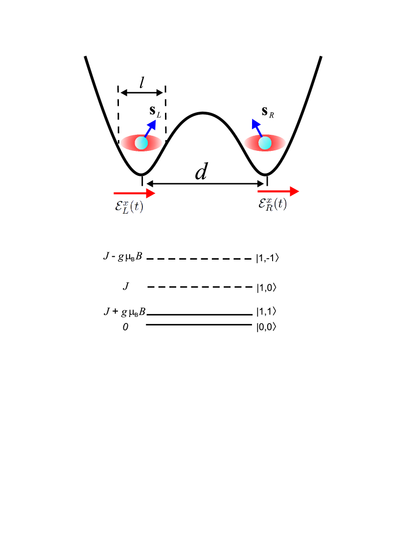
Figure 1: (Color online) (Upper panel) Schematic plot of electrons and applied electric fields in a double quantum dot. (Lower panel) Spin states in the absence of external driving.

In the basis $|0,0\rangle\equiv|1\rangle=(1,0)^{T}$ and $|1,1\rangle\equiv|2\rangle=(0,1)^{T}$, where the $T$ stands for transpose, the total spin-dependent Hamiltonian (neglecting $H_{\text{so}}$-term) becomes

$$H=\frac{\hbar}{2}\left(\begin{array}[]{cc}Z_{1}&X+iY\\ X-iY&Z_{2}\end{array}\right),$$ (9)

where the elements of the matrix are:

$$X = \frac{\sqrt{2}\alpha}{\hbar}\frac{e}{c}(A_{L}^{y}-A_{R}^{y}),$$ (10)

$$Y = -\frac{\sqrt{2}\alpha}{\hbar}\frac{e}{c}(A_{L}^{x}-A_{R}^{x}),$$ (11)

$$Z_{1} = -\frac{3J}{2\hbar},$$ (12)

$$Z_{2} = \frac{1}{\hbar}\left[\frac{J}{2}+2\Delta-2\beta\frac{e}{c}(A_{L}^{x}+A_{R}^{x})\right].$$ (13)

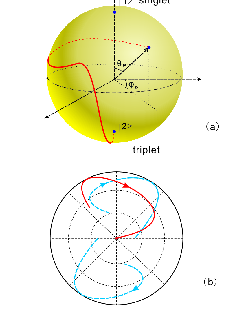
Figure 2: (Color online) (a) Schematic plot of spin control from an arbitrary state to the target state $|2{\rangle}$ on the Bloch sphere, where the north and south poles represent the singlet state $|1{\rangle}=|0,0{\rangle}$ and triplet state $|2{\rangle}=|1,1{\rangle}$. (b) Schematic projection from top view on the $x$-$y$ plane of the auxiliary paths of two eigenstates of the dynamical invariant (dashed blue line), compared to the physical path of state evolution driven by the designed Hamiltonian (solid red line).

Here, unlike the single QD spinQD , counterdiabatic protocol (or quantum transitionless driving) Rice ; Berry09 ; Chen10b could be applied for electric spin controlYue . However, rather than relying on a potentially complicated control of required four parameters, we restrict ourselves to the simplifying assumptions $A_{L}^{y}=A_{R}^{y}=X=0$, which leaves the electric field $x$-components the only controlled function. The gauge is fixed by assuming ${\mathcal{E}}_{L,R}^{x}=0$ for all $t<0$ and $A_{L,R}^{x}(0)=0$ so that the electric fields start to be built up from $t=0$. In the following sections we inversely engineer the time dependence of required electric fields for arbitrary operations by using corresponding invariants of the motion.

III Dynamical invariants and inverse engineering

For completeness we shall first briefly review the Lewis-Riesenfeld invariant theory applied to a two-level system. Specifically for our DQD system we shall then design by two-mode inverse engineering the electric fields to induce a particular transition. A dynamical invariant $I$ of the Hamiltonian $H$ should satisfy

$$\frac{dI(t)}{dt}\equiv\frac{\partial I(t)}{\partial t}+\frac{i}{\hbar}[H(t),I(t)]=0,$$ (14)

so that its expectation values remain constant in time. Parameterizing the Bloch sphere by a polar angle $\theta_{a}(t)\equiv\theta_{a}$ and the azimuthal angle $\varphi_{a}(t)\equiv\varphi_{a}$, we may express the orthogonal eigenstates $|\chi_{\pm}(t){\rangle}$ of the invariant $I(t)$ as

$$|\chi_{+}(t){\rangle} = \left(\begin{array}[]{c}\cos\displaystyle{\frac{\theta_{a}}{2}}e^{i\varphi_{a}}\\ \sin\displaystyle{\frac{\theta_{a}}{2}}\end{array}\right),$$ (17)

$$|\chi_{-}(t){\rangle} = \left(\begin{array}[]{c}\sin\displaystyle{\frac{\theta_{a}}{2}}\\ -\cos\displaystyle{\frac{\theta_{a}}{2}}e^{-i\varphi_{a}}\end{array}\right).$$ (20)

Assuming that $I(t)|\chi_{\pm}(t){\rangle}=\lambda_{\pm}|\chi_{\pm}(t){\rangle}$ with eigenvalues $\lambda_{\pm}=\pm g\mu_{B}B_{c}/2$, we can write the invariant as ChenPRA

$$I(t)=\frac{g\mu_{B}}{2}B_{c}\left(\begin{array}[]{cc}\cos{\theta_{a}}&\sin{\theta_{a}}e^{i\varphi_{a}}\\ \sin{\theta_{a}}e^{-i\varphi_{a}}&-\cos{\theta_{a}}\end{array}\right),$$ (23)

where $B_{c}$ is an arbitrary constant magnetic field to keep $I(t)$ with units of energy. According to Lewis-Riesenfeld theory, the solution of the Schrödinger equation, $i\hbar\partial_{t}\Psi=H(t)\Psi$, is a superposition of orthonormal “dynamical modes” LR , $\Psi(t)=\sum_{n}c_{n}e^{i\gamma_{n}(t)}|\chi_{n}(t){\rangle}$ ($n=\pm$), where $c_{n}$ are time-independent amplitudes and $\gamma_{n}(t)$ are Lewis-Riesenfeld phases,

$$\gamma_{n}\equiv\gamma_{n}(t)=\frac{1}{\hbar}\int^{t}_{0}\langle\chi_{n}(t^{\prime})|i\hbar\frac{\partial}{\partial t^{\prime}}-H(t^{\prime})|\chi_{n}(t^{\prime})\rangle dt^{\prime}.$$ (24)

Substituting Eqs. (9) and (23) into Eq. (14) and combining it with Eq. (24), we may write the Hamiltonian matrix elements in terms of invariant eigenvector angles as

$$X = (\dot{\gamma}_{-}-\dot{\gamma}_{+}-\dot{\varphi}_{a})\sin\theta_{a}\cos\varphi_{a}+\dot{\theta}_{a}\sin\varphi_{a},~{}~{}$$ (25)

$$Y = (\dot{\gamma}_{-}-\dot{\gamma}_{+}-\dot{\varphi}_{a})\sin\theta_{a}\sin\varphi_{a}-\dot{\theta}_{a}\cos\varphi_{a},~{}~{}$$ (26)

$$Z_{1} = -(\dot{\gamma}_{-}+\dot{\gamma}_{+})-\dot{\varphi}_{a}+(\dot{\gamma}_{-}-\dot{\gamma}_{+}-\dot{\varphi}_{a})\cos\theta_{a},~{}~{}~{}$$ (27)

$$Z_{2} = -(\dot{\gamma}_{-}+\dot{\gamma}_{+})+\dot{\varphi}_{a}-(\dot{\gamma}_{-}-\dot{\gamma}_{+}-\dot{\varphi}_{a})\cos\theta_{a},~{}~{}~{}$$ (28)

from which Lewis-Riesenfeld phases are found to obey

$$\dot{\gamma}_{+} = \frac{3J}{4\hbar}+\frac{1}{2}\dot{\theta}_{a}\tan{\frac{\theta_{a}}{2}}\tan\varphi_{a}-\dot{\varphi}_{a},$$ (29)

$$\dot{\gamma}_{-} = \frac{3J}{4\hbar}-\frac{1}{2}\dot{\theta}_{a}\cot{\frac{\theta_{a}}{2}}\tan\varphi_{a},$$ (30)

and the vector potential components take the form

$$A^{x}_{L} = \frac{\hbar c}{2\beta e}\left[\frac{J+\Delta}{\hbar}-\dot{\varphi}_{a}\right.$$

$$-\left.\dot{\theta}_{a}\cot{\theta_{a}}\tan{\varphi_{a}}+\frac{\beta\dot{\theta}_{a}}{\sqrt{2}\alpha}\sec{\varphi_{a}}\right],$$

$$A^{x}_{R} = \frac{\hbar c}{2\beta e}\left[\frac{J+\Delta}{\hbar}-\dot{\varphi}_{a}\right.$$

$$-\left.\dot{\theta}_{a}\cot{\theta_{a}}\tan{\varphi_{a}}-\frac{\beta\dot{\theta}_{a}}{\sqrt{2}\alpha}\sec{\varphi_{a}}\right],$$

when $A^{y}_{L}=A^{y}_{R}=0$ is imposed. Note the possibility of finding divergences when $\varphi_{a}$ is an odd multiple of $\pi/2$ and when $\theta_{a}$ is a multiple of $\pi$.

Once the functions $\theta_{a}(t)$ and $\varphi_{a}(t)$ are known, the electric fields, ${\mathcal{E}}_{L}^{x}(t)=-(1/c)\partial A_{L}^{x}/\partial t$ and ${\mathcal{E}}_{R}^{x}(t)=-(1/c)\partial A_{R}^{x}/\partial t$, can be calculated. As we keep $A_{L,R}^{x}(0)=0$, the following two constraints should hold:

$$\dot{\theta}_{a}(0) = 0,$$ (33)

$$\dot{\varphi}_{a}(0) = \frac{J+\Delta}{\hbar}.$$ (34)

Next, we shall discuss several examples.

IV Transfer an arbitrary initial state to the target one

Suppose that we want to transfer the arbitrary initial state at $t=0$,

$$\Psi(0)=\left(\begin{array}[]{c}\cos{\displaystyle{\frac{\theta_{p}(0)}{2}}}e^{i\varphi_{p}(0)}\\ \sin{\displaystyle{\frac{\theta_{p}(0)}{2}}}\end{array}\right),$$ (37)

to $\Psi(t_{f})=|2{\rangle}$ as the target state at the final time $t=t_{f}$. The polar and azimuthal angles $\theta_{p}\equiv\theta_{p}(t)$ and $\varphi_{p}\equiv\varphi_{p}(t)$, represent the dynamical path on the Bloch sphere of the two-level system, see Fig. 2. In general,

$$\Psi(t)=c_{+}e^{i\gamma_{+}(t)}|\chi_{+}(t){\rangle}+c_{-}e^{i\gamma_{-}(t)}|\chi_{-}(t){\rangle},$$ (38)

where the time-independent coefficients $c_{\pm}={\langle}\chi_{\pm}(0)|\Psi(0){\rangle}$ are given by

$$c_{+} = \cos{\frac{\theta_{a}(0)}{2}}\cos{\frac{\theta_{p}(0)}{2}}e^{i[\varphi_{p}(0)-\varphi_{a}(0)]}$$

$$+\sin{\frac{\theta_{a}(0)}{2}}\sin{\frac{\theta_{p}(0)}{2}},$$

$$c_{-} = \sin{\frac{\theta_{a}(0)}{2}}\cos{\frac{\theta_{p}(0)}{2}}e^{i\varphi_{p}(0)}$$

$$-\cos{\frac{\theta_{a}(0)}{2}}\sin{\frac{\theta_{p}(0)}{2}}e^{i\varphi_{a}(0)}.$$

The time-dependent populations $P_{1}(t)=|{\langle}1|\Psi(t){\rangle}|^{2}$ and $P_{2}(t)=|{\langle}2|\Psi(t){\rangle}|^{2}=1-P_{1}(t)$, can thus be explicitly expressed as

$$P_{1}(t) = \left|c_{+}\cos\frac{\theta_{a}}{2}e^{i(\varphi_{a}+\gamma_{+})}+c_{-}\sin\frac{\theta_{a}}{2}e^{i\gamma_{-}}\right|^{2},$$ (41)

$$P_{2}(t) = \left|c_{+}\sin\frac{\theta_{a}}{2}e^{i\gamma_{+}}-c_{-}\cos\frac{\theta_{a}}{2}e^{-i(\varphi_{a}-\gamma_{-})}\right|^{2}.$$ (42)

To reach the final state $\Psi(t_{f})=|2{\rangle}$, up to a phase factor, the condition $P_{1}(t_{f})=0$ [$P_{2}(t_{f})=1$] should be satisfied, so that we can further set boundary conditions for $\theta_{a}(t_{f})$. Once the boundary conditions for $\theta_{a}$ and $\varphi_{a}$ are fixed, we interpolate $\theta_{a}(t)$ and $\varphi_{a}(t)$, and finally construct the Hamiltonian $H(t)$ and the time-dependent electric fields.

If, for simplicity, $\varphi_{a}(0)$ is set equal to the initial physical angle $\varphi_{p}(0)$, the coefficients $c_{\pm}$ in Eqs. (IV) and (IV) are

$$c_{+} = \cos\frac{\eta}{2},$$ (43)

$$c_{-} = e^{i\varphi_{p}(0)}\sin\frac{\eta}{2},$$ (44)

with $\eta=\theta_{a}(0)-\theta_{p}(0)$. On the Bloch sphere, $\Psi(0)$ and $|\chi_{+}(0){\rangle}$ have the same longitude, while $|\chi_{-}(0){\rangle}$, which is orthogonal to $|\chi_{+}(0){\rangle}$, possesses the azimuthal angle $\pi+\varphi_{p}(0)$. The condition for $P_{2}=1$ [$P_{1}=0$] at the final time $t=t_{f}$, see Eqs. (41) and (42), is

$$1+\cos\theta_{a}(t_{f})\cos\eta+\sin\theta_{a}(t_{f})\sin\eta\cos u(t_{f})=0,$$ (45)

where

$$u(t)=-\int^{t}_{0}\dot{\theta}_{f}(\tau)\frac{\tan\varphi_{a}(\tau)}{\sin\theta_{a}(\tau)}d\tau.$$ (46)

We have used

$$\gamma_{-}(t)-\gamma_{+}(t)=\varphi_{a}(t)-\varphi_{a}(0)+u(t),$$ (47)

which follows from $X=0$, see Eq. (10). We note from Eqs. (43) and (44) that $\eta$ determines the relative weights of the two eigenstates. For two-mode driving, when $\eta$ is not equal to $0$ or $\pi$, Eq. (45) holds only when $\cos u(t_{f})=\pm 1$.

IV.1 Example 1: $\cos u(t_{f})=1$

We choose first $\cos u(t_{f})=1$. In this case, $u(t_{f})=2k\pi$ ($k=0,\pm 1,\pm 2...$) and the condition (45) becomes

$$\cos[\theta_{a}(t_{f})-\eta]=-1,$$ (48)

which gives

$$\theta_{a}(t_{f})=\theta_{a}(0)-\theta_{p}(0)+\pi.$$ (49)

To fulfill Eq. (49) and Eq. (33), we use the second order polynomial Ansatz

$$\theta_{a}(t)=\sum_{j=0}^{2}a_{j}t^{j},$$ (50)

where the coefficients $a_{j}$ can be found with a given $\theta_{a}(0)$. In addition, we interpolate $\varphi_{a}$ by

$$\tan\varphi_{a}(t)=\left(\sum_{j=0}^{2}b_{j}t^{j}\right)\sin\theta_{a}(t),$$ (51)

to avoid singularities in Eq. (46). Here $b_{0}=\tan\varphi_{p}(0)/\sin\theta_{a}(0)$ is obtained from $\varphi_{a}(0)=\varphi_{p}(0)$, and $b_{1}$ and $b_{2}$ can be solved from Eq. (34) and $u(t_{f})=2k\pi$.

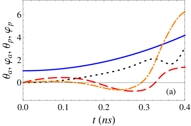
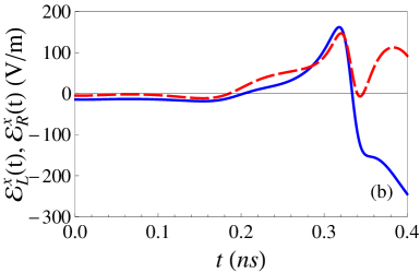
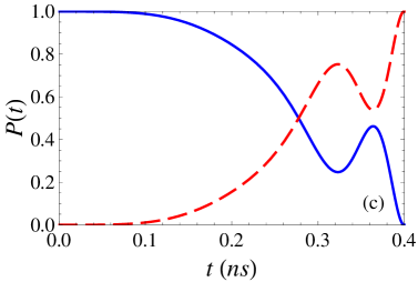
Figure 3: (Color online) Example 1 for two-mode driving with the initial conditions: $\theta_{p}(0)=0$, $\varphi_{p}(0)=0$, $\theta_{a}(0)=\pi/3$, and $\varphi_{a}(0)=\varphi_{p}(0)$. For $u(t_{f})=2\pi$: (a) The two auxiliary angles, $\theta_{a}$ (solid blue line) and $\varphi_{a}$ (dashed red line), determined by Eqs. (50) and (51), compared to the physical polar angle $\theta_{p}$ (dotted black line) and the physical azimuthal angle $\varphi_{p}$ (dot-dashed orange line). (b) The designed electric fields ${\mathcal{E}}^{x}_{L}$ (solid blue line) and ${\mathcal{E}}^{x}_{R}$ (dashed red line). (c) The populations $P_{1}$ (solid blue line) and $P_{2}$ (dashed red line). Parameters: $t_{f}=0.4$ ns, $B_{1}=B_{2}=3.67$ T, $g=-0.44$, $J=0.1$ meV (consequently, $|J+\Delta|/J=0.06$), $\hbar\beta=0.25\times 10^{-6}$ meV$\cdot$cm, and $\alpha=\beta/2$.

Let us consider a population inversion or singlet-triplet transition from the initial state $|1{\rangle}$ (we set $\theta_{p}(0)=0$ and $\varphi_{p}(0)=0$) to final state $|2{\rangle}$ (up to a phase factor) for $t_{f}=0.4$ ns. For this operation time, the relevant energy scale is below $0.01$ meV, much less than the singlet-triplet spitting $J=0.1$ meV, such that transitions to the two higher triplet states do not occur.

If we choose $\theta_{a}(0)=\pi/3$ and $k=1$, the functions of $\theta_{a}(t)$ and $\varphi_{a}(t)$ can be calculated from Eqs. (50) and (51), as shown in Fig. 3 (a). The corresponding electric fields are depicted in Fig. 3 (b). The population dynamics is numerically calculated by solving the time-dependent Schrödinger equation. Fig. 3 (c) demonstrates that the spin state evolves from the initial state $|1{\rangle}$ to final one $|2{\rangle}$, up to a phase factor $\exp[i\varphi_{p}(t_{f})]$, for the fixed time $t_{f}=0.4$ ns.  The physical angles $\theta_{p}(t)$ and $\varphi_{p}(t)$ corresponding to the trajectory of the spin state on the Bloch sphere are also shown in Fig. 3 (a).

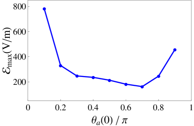
Figure 4: (Color online) Maximal value ${\mathcal{E}}_{\max}$ of the electric fields versus the initial boundary condition $\theta_{a}(0)$ in the example 1, with Eqs. (50) and (51). Other parameters are the same as those in Fig. 3.

The two-mode driving scheme provides flexibility to pick up different boundary conditions for $\theta_{a}$ and $\varphi_{a}$, so as to minimize the fields. To demonstrate this, we choose different initial values of $\theta_{a}(0)$. The maximal absolute value ${\mathcal{E}}_{\max}$ of applied electric fields, ${\mathcal{E}}^{x}_{L}$ and ${\mathcal{E}}^{x}_{R}$, that is, ${\mathcal{E}}_{\max}=\max(|{\mathcal{E}}^{x}_{L}|,|{\mathcal{E}}^{x}_{R}|)$, can be decreased by choosing a suitable $\theta_{a}(0)$, as shown in Fig. 4. Note that each two-mode scheme is equivalent to a single-mode one, when the physical polar and azimuthal angles, $\theta_{p}$ and $\varphi_{p}$, are reinterpreted  by the two auxiliary angles $\theta_{a}$ and $\varphi_{a}$ for designing the eigenstates of the invariant. However, the functions of these angles are generally not simple.

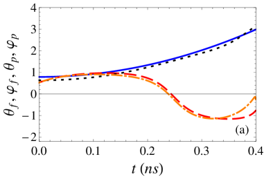
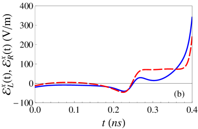
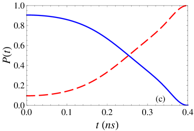
Figure 5: (Color online) Example 2 for two-mode driving with initial conditions: $\theta_{p}(0)=\pi/5$, $\varphi_{p}(0)=\pi/6$, $\theta_{a}(0)=\pi/4$, and $\varphi_{a}(0)=\varphi_{p}(0)$. For $u(t_{f})=\pi$: (a) The two auxiliary angles, $\theta_{a}$ (solid blue line) and $\varphi_{a}$ (dashed red line), determined by Eqs. (50) and (51), compared to the physical polar angle $\theta_{p}$ (dotted black line) and the physical azimuthal angle $\varphi_{p}$ (dot-dashed orange line). (b) The designed electric fields ${\mathcal{E}}^{x}_{L}$ (solid blue line) and ${\mathcal{E}}^{x}_{R}$ (red dashed line). (c) The populations $P_{1}$ (solid blue line) and $P_{2}$ (dashed red line). Other parameters are the same as in Fig. 3.

IV.2 Example 2: $\cos u(t_{f})=-1$

For the choice $\cos u(t_{f})=-1$, we have $u(t_{f})=(2k-1)\pi$ ($k=0,\pm 1,\pm 2...$) and the condition for $P_{2}(t_{f})=1$ becomes

$$\cos[\theta_{a}(t_{f})+\eta]=-1,$$ (52)

which results in

$$\theta_{a}(t_{f})=-\theta_{a}(0)+\theta_{p}(0)+\pi.$$ (53)

In the example 2, we want to manipulate the spin state from an arbitrary state to $|2{\rangle}$ (up to a phase factor). We apply the same forms of $\theta_{a}$ and $\varphi_{a}$ as before [see Eqs. (50) and (51)], and choose a different initial state $\theta_{p}(0)=\pi/5$, $\varphi_{p}(0)=\pi/6$, and $\theta_{a}(0)=\pi/4$. For the fixed time $t_{f}=0.4$ ns, the two auxiliary angles $\theta_{a}$ and $\varphi_{a}$ are determined by Eqs. (50) and (51), as seen in Fig. 5 (a), where the physical angles of $\theta_{p}$ and $\varphi_{p}$ are compared. The electric fields, ${\mathcal{E}}^{x}_{L}$ and ${\mathcal{E}}^{x}_{R}$ are shown in Fig. 5 (b). The populations are represented in Fig. 5 (c), in which the target state $|2{\rangle}$ is achieved at final time $t_{f}=0.4$ ns.

V Transfer the initial state to an arbitrary state

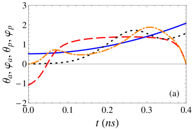
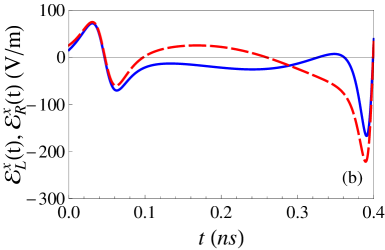
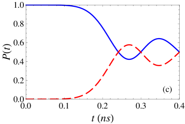
Figure 6: (Color online) Example 3 for two-mode driving with the conditions at the final state: $\theta_{p}(t_{f})=\pi/2$, $\varphi_{p}(t_{f})=0$, $\theta_{a}(0)=\pi/6$. For $u(t_{f})=-2\pi$: (a) The two auxiliary angles, $\theta_{a}$ (solid blue line) and $\varphi_{a}$ (dashed red line), compared to the physical polar angle $\theta_{p}$ (dotted black line) and the physical azimuthal angle $\varphi_{p}$ (dot-dashed orange line). (b) The designed electric fields ${\mathcal{E}}^{x}_{L}$ (solid blue line) and ${\mathcal{E}}^{x}_{R}$ (dashed red line). (c) The populations $P_{1}$ (solid blue line) and $P_{2}$ (dashed red line). Other parameters are the same as in Fig. 3.

We consider now a transition from $\Psi(0)=|1{\rangle}$ to an arbitrary state at $t=t_{f}$,

$$\Psi(t_{f})=\left(\begin{array}[]{c}\cos{\displaystyle{\frac{\theta_{p}(t_{f})}{2}}}e^{i\varphi_{p}(t_{f})}\\ \sin{\displaystyle{\frac{\theta_{p}(t_{f})}{2}}}\end{array}\right).$$ (56)

Choosing $\varphi_{p}(t_{f})=\varphi_{a}(t_{f})$ for simplicity, the time-independent coefficients  $c_{\pm}=e^{-i\gamma_{\pm}(t_{f})}{\langle}\chi_{\pm}(t_{f})|\Psi(t_{f}){\rangle}$ are expressed as

$$c_{+} = e^{-i\gamma_{+}(t_{f})}\cos\frac{\zeta}{2},$$ (57)

$$c_{-} = e^{-i[\gamma_{-}(t_{f})-\varphi_{a}(t_{f})]}\sin\frac{\zeta}{2},$$ (58)

where $\zeta=\theta_{a}(t_{f})-\theta_{p}(t_{f})$. As the initial state is $|1{\rangle}$ (up to some phase factor), $P_{1}(0)$=1 [$P_{2}(0)=0$] gives the following condition,

$$1-\cos\zeta\cos\theta_{a}(0)-\sin\zeta\sin\theta_{a}(0)\cos u(t_{f})=0.$$ (59)

Similarly to the case of state transfer from an arbitrary state to $|2{\rangle}$, Eq. (59) holds when $\cos u(t_{f})=\pm 1$. Taking $\cos u(t_{f})=1$ leads to

$$\cos[\zeta-\theta_{a}(0)]=1,$$ (60)

and

$$\theta_{a}(t_{f})=\theta_{p}(t_{f})+\theta_{a}(0).$$ (61)

We choose the same second-order polynomial Ansatz for $\theta_{a}(t)$ as in Eq. (50). With a given $\theta_{a}(0)$, the coefficients $a_{j}$ can be solved from the constraint $\dot{\theta}_{a}(0)=0$ and Eq. (61). Again we set the same form of $\varphi_{a}(t)$ as in Eq. (51). The $b_{j}$ follow from the preconditions $\varphi_{a}(t_{f})=\varphi_{p}(t_{f})$, the constraint $\dot{\varphi}(0)=(J+\Delta)/\hbar$, and $u(t_{f})=2k\pi$ ($k=0,\pm 1,\pm 2...$).

In example 3, we show the state transfer from $|1{\rangle}$ to $\Psi(t_{f})=(|1{\rangle}+|2{\rangle})/\sqrt{2}$, that is, $\theta_{p}(t_{f})=\pi/2$ and $\varphi_{p}(t_{f})=0$. For $k=-1$, the auxiliary angles $\theta_{a}$, $\varphi_{a}$ and the physical angles $\theta_{p}$ and $\varphi_{p}$ are displayed in Fig. 6 (a). This transition realizes a fast Hadamard gate Nielsenbook since $|2{\rangle}$ becomes $(|1{\rangle}-|2{\rangle})/\sqrt{2}$.

VI Conclusion

We have studied the possibility to manipulate by electric fields transitions in a singlet-triplet subspace of a two-electron double quantum dot in the presence of spin-orbit coupling. By using inverse engineering based on Lewis-Riesenfeld invariants, we have designed the Hamiltonians that allow for a fast spin manipulation on a desired timescale. We have applied two-mode driving using both eigenstates of the dynamical invariant and the time-dependent difference in their phases. Generally, any fast transition protocol can be equivalently designed by using a single-mode driving. However, the two-mode approach is more flexible and provides simpler Ansantzes for the eigenstates of the dynamical invariants. This technique has proven useful to minimize the electric fields necessary to perform the spin operations. This approach can as well be used in other two-level quantum systems, such as two-level atoms Chen10b , Bose-Einstein condensates in accelerated optical lattices Oliver , and nitrogen-vacancy (NV) center spin in diamond Zhang , for engineering their quantum dynamics.

References

- (1) L. Allen and J. H. Eberly, Optical Resonance and Two-level Atoms (Dover, New York, 1987).
- (2) K. Bergmann, H. Theuer, and B. W. Shore, Rev. Mod. Phys. 70, 1003 (1998).
- (3) N. V. Vitanov, T. Halfmann, B. W. Shore, and K. Bergmann, Ann. Rev. Phys. Chem. 52, 763 (2001).
- (4) P. Král, I. Thanopulos, and M. Shapiro, Rev. Mod. Phys. 79, 53 (2007).
- (5) M. Saffman, T. G. Walker, and K. Mølmer, Rev. Mod. Phys. 82, 2313 (2010).
- (6) M. Demirplak and S. A. Rice, J. Phys. Chem. A 107, 9937 (2003); J. Phys. Chem. B 109, 6838 (2005); J. Chem. Phys. 129, 154111 (2008).
- (7) M. V. Berry, J. Phys. A 42, 365303 (2009).
- (8) X. Chen, A. Ruschhaupt, S. Schmidt, A. del Campo, D. Guéry-Odelin, and J. G. Muga, Phys. Rev. Lett. 104, 063002 (2010).
- (9) X. Chen, I. Lizuain, A. Ruschhaupt, D. Guéry-Odelin, and J. G. Muga, Phys. Rev. Lett. 105, 123003 (2010).
- (10) X. Chen, E. Torrontegui, and J. G. Muga, Phys. Rev. A 83, 062116 (2011).
- (11) E. Torrontegui, S. Ibáñez, X. Chen, A. Ruschhaupt, D. Guéry-Odelin, and J. G. Muga, Phys. Rev. A 83, 013415 (2011).
- (12) X. Chen, E. Torrontegui, D. Stefanatos, J.-S. Li, and J. G. Muga, Phys. Rev. A 84, 043415 (2011).
- (13) S. Ibáñez, X. Chen, E. Torrontegui, J. G. Muga, and A. Ruschhaupt, Phys. Rev. Lett. 109, 100403 (2012).
- (14) S. Masuda and K. Nakamura, Proc. R. Soc. A 466, 1135 (2010); Phys. Rev. A 84, 043434 (2011).
- (15) E. Torrontegui, S. Ibáñez, S. Martínez-Garaot, M. Modugno, A. del Campo, D. Guéry-Odelin, A. Ruschhaupt, X. Chen, and J. G. Muga, arXiv:1212.6343, Adv. At. Mol. Opt. Phys., to be published (2013).
- (16) G. Burkard, D. Loss, and D. P. DiVincenzo, Phys. Rev. B, 59, 2070 (1999).
- (17) L. Jacak, P. Hawrylak, and A. Wójs, Quantum Dots (Springer, Berlin, 1997).
- (18) J. Medford, J. Beil, J. M. Taylor, S. D. Bartlett, A. C. Doherty, E. I. Rashba, D. P. DiVincenzo, H. Lu, A. C. Gossard, and C. M. Marcus, arXiv:1302.1933.
- (19) C. Kloeffel and D. Loss, Annu. Rev. Condens. Matter Phys. 4, 10.1-10.31 (2013).
- (20) Y. Ban, X. Chen, E. Ya. Sherman, and J. G. Muga, Phys. Rev. Lett. 109, 206602 (2012).
- (21) E. I. Rashba and Al. L. Efros, Phys. Rev. Lett. 91, 126405 (2003).
- (22) F. H. L. Koppens, C. Buizert, K. J. Tielrooij, I. T. Vink, K. C. Nowack, T. Meunier, L. P. Kouwenhoven, and L. M. K. Vandersypen, Nature 442, 766 (2006).
- (23) K. C. Nowack, F. H. L. Koppens, Yu. V. Nazarov, and L. M. K. Vandersypen, Science 318, 1430 (2007).
- (24) D. Stepanenko, M. Rudner, B. I. Halperin, and D. Loss, Phys. Rev. B 85, 075416 (2012).
- (25) R. Hanson, L. P. Kouwenhoven, J. R. Petta, S. Tarucha, and L. M. K. Vandersypen, Rev. Mod. Phys. 79, 1217 (2007).
- (26) J. R. Petta, A. C. Johnson, J. M. Taylor, E. A. Laird, A. Yacoby, M. D. Lukin, C. M. Marcus, M. P. Hanson, and A. C. Gossard, Science 309, 2180 (2005).
- (27) X. Chen and J. G. Muga, Phys. Rev. A 86, 033405 (2012).
- (28) F. R. Waugh, M. J. Berry, D. J. Mar, R. M. Westervelt, K. L. Campman, and A. C. Gossard, Phys. Rev. Lett. 75, 705 (1995); C. Livermore, C. H. Crouch, R. M. Westervelt, K. L. Campman, and A. C. Gossard, Science 274, 1332 (1996).
- (29) P. Fazekas Lecture Notes on Electron Correlation and Magnetism (Series in Modern Condensed Matter Physics), World Scientific, Singapore, (1999).
- (30) T. Hassenkam, S. Pedersen, K. Baklanov, A. Kristensen, C. B. Sorensen, P. E. Lindelof, F. G. Pikus, and G. E. Pikus, Phys. Rev. B 55, 9298 (1997).
- (31) V. N. Golovach, M. Borhani, and D. Loss, Phys. Rev. B 74, 165319 (2006).
- (32) M. P. Nowak, B. Szafran, and F. M. Peeters, Phys. Rev. B 86, 125428 (2012).
- (33) Y. Ban, arXiv:1212.3294.
- (34) H. R. Lewis and W. B. Riesenfeld, J. Math. Phys. 10, 1458 (1969).
- (35) M. A. Nielsen, and I. L. Chuang, Quantum computation and quantum information, Cambridge University Press, Cambridge (2000).
- (36) M. G. Bason, M. Viteau, N. Malossi, P. Huillery, E. Arimondo, D. Ciampini, R. Fazio, V. Giovannetti, R. Mannella, and O. Morsch, Nat. Phys. 8, 147 (2012).
- (37) J.-F. Zhang, J. H. Shim, I. Niemeyer, T. Taniguchi, T. Teraji, H. Abe, S. Onoda, T. Yamamoto, T. Ohshima, J. Isoya, and D. Suter, Phys. Rev. Lett. 110, 240501 (2013).