Primary 62H05, 62G35. Secondary 62-09, G2H25, G2H30.

Affine equivariance, asymptotic theory, breakdown point, eigenprojections, elliptical distributions, principal components, relative efficiency, robustness, spatial sign covariance matrix, Tyler’s scatter matrix.

THE ASYMPTOTIC INADMISSIBILITY OF THE SPATIAL SIGN COVARIANCE MATRIX
FOR ELLIPTICALLY SYMMETRIC DISTRIBUTIONS

Andrew F. Magyar and David E. Tyler

The United States Census Bureau and Rutgers University

A.F. MAGYAR AND D.E. TYLER

INADMISSIBILITY OF TE SPATIAL SIGN COVARIANCE MATRIX

ABSTRACT

The asymptotic efficiency of the spatial sign covariance matrix (SSCM) relative to affine equivariant estimates of scatter is studied in detail. In particular, the SSCM is shown to be asymptoticaly inadmissible, i.e.  the asymptotic variance-covariance matrix of the consistency corrected SSCM is uniformly smaller than that of its affine equivariant counterpart, namely Tyler’s scatter matrix. Although the SSCM has often been recommended when one is interested in principal components analysis, the degree of the inefficiency of the SSCM is shown to be most severe in situations where principal components are of most interest. A finite sample simulation shows the inefficiency of the SSCM also holds for small sample sizes, and that the asymptotic relative efficiency is a good approximation to the finite sample efficiency for relatively modest sample sizes.

3

1 Introduction

Multivariate procedures are implemented to help understand the relationships between several quantitative variables of interest. The most commonly used methods rely heavily on the sample variance-covariance matrix. It is now well known that the sample variance-covariance matrix is highly non-robust, being extremely sensitive to outliers and being very inefficient at longer tailed distributions. Consequently, there have been many proposed robust alternatives to the sample variance-covariance matrix, such as the $M$-estimates (Maronna, 1976; Huber, 1977), the minimum volume ellipsoid and the minimum covariance determinant estimates (Rousseeuw, 1985), the Stahel-Donoho estimates (Stahel, 1981; Donoho, 1982), the $S$-estimates (Davies, 1987; Lopuhaä, 1989), the P-estimates (Maronna et al., 1992; Tyler, 1994), $CM$-estimates (Kent & Tyler, 1996) and the $MM$-estimates (Tatsuoka & Tyler, 2000; Tyler, 2002). All of these estimates of scatter are affine equivariant, and except for the $M$-estimates they all have high breakdown points. On the other hand, the computations of $M$-estimates are relatively easy and can be done via a simple IRLS algorithm, whereas the high breakdown point scatter estimates are computationally intensive, especially for large samples and/or high dimensional data sets, and are usually computed via approximate or probabilistic algorithms.

Due to the computational complexity of high breakdown point affine equivariant estimates of multivariate scatter, there has been recent interest in high breakdown point estimates of scatter which are not affine equivariant but are computationally easy. One such estimate is the spatial sign covariance matrix, hereafter referred to as SSCM. The earliest often cited references to this estimate is Locantore et al. (1999), though the name SSCM was introduced in Visuri et al. (2000). The SSCM is often recommended as a fast and easy high breakdown point method; see e.g. Locantore et al. (1999) and the recent book by Maronna et al. (2006). In particular, since it is orthogonally equivariant, the SSCM has been recommended in cases where only orthogonal equivariance and not full affine equivariance is needed, such as in principal components analysis.

The lack of affine equivariance of the SSCM arises since it is defined by down-weighing observations based upon their Euclidean distances from an estimated center of the data set. When the data is presumed to arise from a multivariate normal distribution or more generally from an elliptically symmetric distribution, one might conjecture that the SSCM would be relatively inefficient whenever the elliptical distribution is far from spherical, i.e. when the components of the multivariate vector are highly correlated. This can be problematic since one usually implements multivariate procedures in situations where one suspects strong correlations between the variables, as is the case when one does a principal components analysis. Our goal here is then to study the efficiency of the SSCM under general covariance structures.

An important property of the SSCM is that its asymptotic distribution does not depend on the particular elliptical family being sampled. This is also true for the finite sample distribution of the SSCM when the center of symmetry of the elliptical distribution is known. An affine equivariant estimate possessing this same property is the distribution free M-estimate of scatter proposed by Tyler (1987a), commonly referred to as Tyler’s scatter matrix. This scatter matrix can be considered an affine equivariant version of the SSCM and so for our purposes here we abbreviate it ASSCM. The asymptotic relative efficiency (ARE) of the SSCM to an affine equivariant estimate of scatter, say $\widehat{\boldsymbol{\Gamma}}$, can then be factored into the ARE of the SSCM to the ASSCM and the ARE of the ASSCM to $\widehat{\boldsymbol{\Gamma}}$. For an elliptically symmetric distribution, the first factor depends only on the underlying covariance structure and not on the particular elliptical family, whereas the second factor depends only on the particular elliptical family and not on the underlying covariance structure. Hence, the ASSCM serves as a convenient benchmark for understanding the effect the lack of affine equivariance has on the efficiency of SSCM for varying covariance structures.

In section 3, we show that our conjecture regarding the inefficiency of the SSCM is indeed true. It is shown the performance of the ASSCM dominates that of the SSCM in that the ARE of the SSCM to the ASSCM is never greater than one regardless of the underlying covariance structure and can approach zero when the component variables are highly correlated. The form of the ARE is complicated, but in special cases it can be expressed in terms of the Gauss hypergeometric functions. A simulation study, presented in section 4, shows that the advantage of the ASSCM over the SSCM holds for relatively small sample sizes and that the asymptotic results are quit accurate even for modest sample sizes. Some technical results and proof are reserved for section 6, an appendix. The following section gives some needed background information on elliptical distributions, affine equivariance, the spatial sign covariance matrix and Tyler’s scatter matrix, as well as sets up the notation for the paper.

2 Preliminaries

2.1 Elliptical distributions and equivariance

Elliptically symmetric distributions provide a simple generalization of the multivariate normal distribution and are often used to ascertain how multivariate statistical methods perform outside of the normal family. An elliptically symmetric distribution in $\mathbb{R}^{d}$ is defined to be one arising from an affine transformation of a spherically symmetric distribution, i.e. if $\boldsymbol{z}\sim_{\mathcal{D}}\boldsymbol{Q}\boldsymbol{z}$ for any $d\times d$ orthogonal matrix $\boldsymbol{Q}$, then the distribution of $\boldsymbol{x}=\boldsymbol{A}\boldsymbol{z}+\boldsymbol{\mu}$ is said to have an elliptically symmetric distribution with center $\boldsymbol{\mu}\in\mathbb{R}^{d}$ and scatter matrix $\boldsymbol{\Gamma}=\boldsymbol{A}\boldsymbol{A}^{T}$, see e.g. section 13.2 in Bilodeau & Brenner (1999). The distribution of $\boldsymbol{x}$ is characterized by $\boldsymbol{\mu}$, $\boldsymbol{\Gamma}$ and the distribution of $\boldsymbol{z}$. The distribution of $\boldsymbol{z}$ itself can be characterized as $\boldsymbol{z}\sim_{\mathcal{D}}R_{G}\boldsymbol{u}_{d}$, with $\boldsymbol{u}_{d}$ having a uniform distribution on the unit $d$-dimensional sphere independent of its radial component $R_{G}$, a non-negative random variable with distribution function $G$. In particular, $(\boldsymbol{u}_{d},R_{G})\sim_{\mathcal{D}}(\boldsymbol{z}/\|\boldsymbol{z}\|,\|\boldsymbol{z}\|)$, where the norm refers to the usual Euclidean norm in $\mathbb{R}^{d}$, i.e. $\|\boldsymbol{z}\|=\sqrt{\boldsymbol{z}^{T}\boldsymbol{z}}$. Thus, we denote the distribution of

$$\boldsymbol{x}\sim_{\mathcal{D}}R_{G}\boldsymbol{\Gamma}^{1/2}\boldsymbol{u}_{d}+\boldsymbol{\mu}$$ (1)

by $\mathcal{E}_{d}(\boldsymbol{\mu},\boldsymbol{\Gamma};G)$, where $\boldsymbol{\Gamma}^{1/2}$ refers to the unique positive definite square root of $\boldsymbol{\Gamma}$. If the distribution of $\boldsymbol{x}$ is also absolutely continuous, then like the multivariate normal distribution, its density has concentric elliptical contours, with a density of the form

$$f\left(\boldsymbol{x};\boldsymbol{\mu},\boldsymbol{\Gamma},g\right)=det\left(\boldsymbol{\Gamma}\right)^{-\frac{1}{2}}g\left(\left(\boldsymbol{x}-\boldsymbol{\mu}\right)^{T}\boldsymbol{\Gamma}^{-1}\left(\boldsymbol{x}-\boldsymbol{\mu}\right)\right),$$ (2)

for $\boldsymbol{x}\in\mathbb{R}^{d}$, where $g$ is some non-negative function and $\boldsymbol{\Gamma}\in\mathcal{P}_{d}$, the class of $d\times d$ symmetric positive definite matrices. The relationship between $g$ and $G$ is $G^{\prime}(r)=a_{d}r^{d-1}g(r^{2})$ with the constant $a_{d}=2\pi^{d/2}/\Gamma\left(d/2\right)$, where the non-bold $\Gamma$ refers to the usual gamma function.

Note that the scatter parameter $\boldsymbol{\Gamma}$ is only well defined up to a scalar multiple, i.e. if $\boldsymbol{\Gamma}$ satisfies the definition of a scatter matrix for a given elliptically symmetric distribution, then $\lambda\boldsymbol{\Gamma}$ also does for any $\lambda>0$. If no restrictions are placed on the function $G$, then the parameter $\boldsymbol{\Gamma}$ is confounded with $G$. If $\boldsymbol{x}$ possesses first moments, then $\boldsymbol{\mu}=E[\boldsymbol{x}]$, and if it possesses second moments, then $\boldsymbol{\Gamma}\propto\boldsymbol{\Sigma}$, the variance-covariance matrix, or more specifically $\boldsymbol{\Sigma}=\lambda(G)\boldsymbol{\Gamma}$ with $\lambda(G)=E[R_{G}^{2}]/d$ .

The parameters of an elliptically symmetric distribution are affinely equivariant. That is, if $\boldsymbol{x}\sim_{\mathcal{D}}\mathcal{E}_{d}(\boldsymbol{\mu},\boldsymbol{\Gamma};G)$, then $\boldsymbol{B}\boldsymbol{x}+\boldsymbol{b}\sim_{\mathcal{D}}\mathcal{E}_{d}(\boldsymbol{B}\boldsymbol{\mu}+\boldsymbol{b},\boldsymbol{B}\boldsymbol{\Gamma}\boldsymbol{B}^{T};G)$ for any non-singular $d\times d$ matrix $\boldsymbol{B}$ and any vector $\boldsymbol{b}\in\mathbb{R}^{d}$. Consequently, the maximum likelihood estimates for the parameters of an elliptically symmetric distribution based on a given function $G$ are affinely equivariant. Given a $d$-dimensional sample $\boldsymbol{x}_{1},\ldots,\boldsymbol{x}_{n}$, estimates of $\boldsymbol{\mu}$ and $\boldsymbol{\Gamma}$ are said to be affinely equivariant if an affine transformation of the data $\boldsymbol{x}_{i}\rightarrow\boldsymbol{B}\boldsymbol{x}_{i}+\boldsymbol{b}$ for $i=1,\ldots,n$ induces on the estimates the transformations $\widehat{\boldsymbol{\mu}}\rightarrow\boldsymbol{B}\widehat{\boldsymbol{\mu}}+\boldsymbol{b}$ and $\widehat{\boldsymbol{\Gamma}}\rightarrow\boldsymbol{B}\widehat{\boldsymbol{\Gamma}}\boldsymbol{B}^{T}$. In addition to the maximum likelihood estimates associated with elliptically symmetric distributions, which include the sample mean vector and the sample covariance matrix, many proposed robust estimates of multivariate location and scatter, such as the multivariate M-estimates, are affinely equivariant.

The covariance matrix, if it exists, of an affine equivariant estimate of scatter under random sampling from an $\mathcal{E}_{d}(\boldsymbol{\mu},\boldsymbol{\Gamma};G)$ distribution has a relatively simple form, namely

$$var(vec\{\widehat{\boldsymbol{\Gamma}}\})=\sigma_{1,n,\widehat{\boldsymbol{\Gamma}},G}(\boldsymbol{I}_{d^{2}}+\mathcal{K}_{d,d})(\boldsymbol{\Gamma}\otimes\boldsymbol{\Gamma})+\sigma_{2,n,\widehat{\boldsymbol{\Gamma}},G}vec(\boldsymbol{\Gamma})vec(\boldsymbol{\Gamma})^{T}.$$ (3)

The notation $vec(\boldsymbol{A})$ refers to the $pq$-dimensional vector obtained from stacking the columns of the $p\times q$ dimensional matrix $\boldsymbol{A}$, $\mathcal{K}_{d,d}$ refers to the $d^{2}\times d^{2}$ commutation matrix, and $\otimes$ refers to the Kronecker product. This notation is reviewed in Appendix 6.1. The terms $\sigma_{1,n,\widehat{\boldsymbol{\Gamma}},G}$ and $\sigma_{2,n,\widehat{\boldsymbol{\Gamma}},G}$ are scalars that depend on the sample size, the particular estimate $\widehat{\boldsymbol{\Gamma}}$ and on the underlying family of elliptical distribution, i.e. on $G$, but not on $\boldsymbol{\mu}$ or $\boldsymbol{\Gamma}$, see Tyler (1983) for more details. When focusing on the shape of the scatter parameter, i.e. on $\boldsymbol{\Gamma}$ up to a scalar multiple, the second scalar becomes unimportant, at least asymptotically. That is, if $\widehat{\boldsymbol{\Gamma}}$ converges in probability and is asymptotically normal, then if the function $\mathcal{H}$ is such that $\mathcal{H}(\boldsymbol{\Gamma})=\mathcal{H}(\beta\boldsymbol{\Gamma})$ for any $\beta>0$, e.g. $\mathcal{H}(\boldsymbol{\Gamma})=vec(\boldsymbol{\Gamma})/\mbox{trace}(\boldsymbol{\Gamma})$, then

$$\sqrt{n}\{\mathcal{\mathcal{H}}(\widehat{\boldsymbol{\Gamma}})-\mathcal{\mathcal{H}}(\boldsymbol{\Gamma})\}\rightarrow_{\mathcal{D}}Normal_{p}\left(\boldsymbol{0},\sigma_{1,\widehat{\boldsymbol{\Gamma}},G}\mathcal{M}(\boldsymbol{\Gamma})\right),$$ (4)

where $p$ is the dimension of $\mathcal{H}$, $\mathcal{M}$ is a function dependent on $\mathcal{H}$ with $\mathcal{M}(\beta\boldsymbol{\Gamma})=\mathcal{M}(\boldsymbol{\Gamma})$ for any $\beta>0$, and $\sigma_{1,\widehat{\boldsymbol{\Gamma}},G}$ is again a scalar dependent only on the particular estimate and on $G$. Thus, the asymptotic relative efficiency at $\mathcal{E}_{d}(\boldsymbol{\mu},\boldsymbol{\Gamma};G)$ of any shape component based on one affine equivariant asymptoptically normal estimate of scatter versus another reduces to the scalar

$$ARE\left(\mathcal{H}(\widehat{\boldsymbol{\Gamma}}_{1}),\mathcal{H}(\widehat{\boldsymbol{\Gamma}}_{2})\right)=\frac{\sigma_{1,\widehat{\boldsymbol{\Gamma}}_{2},G}}{\sigma_{1,\widehat{\boldsymbol{\Gamma}}_{1},G}},$$ (5)

which is not dependent on the shape function $\mathcal{H}$ nor on the parameters $\boldsymbol{\mu}$ and $\boldsymbol{\Gamma}$. We again refer the reader to Tyler (1983) for more details.

2.2 Spatial Sign Covariance Matrix

Given a $d$-dimensional sample $\textbf{x}_{1},\ldots,\textbf{x}_{n}$, the spatial sign covariance matrix, or SSCM, about a point $\boldsymbol{\mu}$ is defined to be

$$\widehat{\boldsymbol{\mathcal{S}}}(\boldsymbol{\mu})=\frac{1}{n}\sum^{n}_{i=1}\frac{\left(\boldsymbol{x}_{i}-\boldsymbol{\mu}\right)\left(\boldsymbol{x}_{i}-\boldsymbol{\mu}\right)^{T}}{\left(\boldsymbol{x}_{i}-\boldsymbol{\mu}\right)^{T}\left(\boldsymbol{x}_{i}-\boldsymbol{\mu}\right)}=\frac{1}{n}\sum^{n}_{i=1}\boldsymbol{\theta}_{i}\boldsymbol{\theta}_{i}^{T},$$ (6)

where $\boldsymbol{\theta}_{i}=(\boldsymbol{x}_{i}-\boldsymbol{\mu})/\|\boldsymbol{x}_{i}-\boldsymbol{\mu}\|$. Note that by definition, $\mbox{trace}\{\widehat{\boldsymbol{\mathcal{S}}}(\boldsymbol{\mu})\}=1$. Under general random sampling $\boldsymbol{\Xi}=E\left[\widehat{\boldsymbol{\mathcal{S}}}(\boldsymbol{\mu})\right]=E\left[\boldsymbol{\theta}\boldsymbol{\theta}^{T}\right]$, where $\boldsymbol{\theta}=(\boldsymbol{x}-\boldsymbol{\mu})/\|\boldsymbol{x}-\boldsymbol{\mu}\|$, and by the law of large numbers $\widehat{\boldsymbol{\mathcal{S}}}(\boldsymbol{\mu})$ is consistent for $\boldsymbol{\Xi}$. Also, since $\|\boldsymbol{\theta}\|=1$, the central limit theorem immediately gives

$$\sqrt{n}~{}vec\{\widehat{\boldsymbol{\mathcal{S}}}(\boldsymbol{\mu})-\boldsymbol{\Xi}\}\rightarrow_{\mathcal{D}}Normal_{d^{2}}\left(\boldsymbol{0},\boldsymbol{\mathcal{V}}_{\mathcal{S}}\right),$$ (7)

where $\boldsymbol{\mathcal{V}}_{\mathcal{S}}=var\left(vec\{\boldsymbol{\theta}\boldsymbol{\theta}^{T}\}\right)=var\left(\boldsymbol{\theta}\otimes\boldsymbol{\theta}\right)=\left(E[\boldsymbol{\theta}\boldsymbol{\theta}^{T}\otimes\boldsymbol{\theta}\boldsymbol{\theta}^{T}]-vec(\boldsymbol{\Xi})vec(\boldsymbol{\Xi})^{T}\right)$. In practice, $\boldsymbol{\mu}$ is usually estimated, say by $\widehat{\boldsymbol{\mu}}_{n}$. The asymptotic distribution of the SSCM when the center is estimated, that is for $\widehat{\boldsymbol{\mathcal{S}}}(\widehat{\boldsymbol{\mu}}_{n})$, which we hereafter abbreviate as $\widehat{\boldsymbol{\mathcal{S}}}_{n}$ has only recently been obtained, see Dürre et al. (2013). As the following lemma shows, under mild conditions the asymptotic distribution of $\widehat{\boldsymbol{\mathcal{S}}}_{n}$ is the same as that of $\widehat{\boldsymbol{\mathcal{S}}}(\boldsymbol{\mu})$. Since the definition of $\widehat{\boldsymbol{\mathcal{S}}}_{n}$ depends on the directions of $\boldsymbol{x}_{i}-\widehat{\boldsymbol{\mu}}_{n}$, it is not surprising to note that the distribution of $\boldsymbol{x}_{i}$ cannot be too concentrated about $\widehat{\boldsymbol{\mu}}_{n}$.

Lemma 2.1

Suppose $\boldsymbol{x}\in\mathbb{R}^{k}$ is a continuous random vector whose distribution is symmetric about $\boldsymbol{\mu}$, i.e. $(\boldsymbol{x}-\boldsymbol{\mu})\sim_{\mathcal{D}}-(\boldsymbol{x}-\boldsymbol{\mu})$, and such that $E[\|\boldsymbol{x}-\boldsymbol{\mu}\|^{-3/2}]<\infty$. For a $k$-dimensional random sample $\boldsymbol{x}_{1},\ldots,\boldsymbol{x}_{n}$ of the random vector $\boldsymbol{x}$, suppose $\sqrt{n}(\widehat{\boldsymbol{\mu}}_{n}-\boldsymbol{\mu})=O_{\mathcal{P}}(1)$, then $\sqrt{n}\{\widehat{\boldsymbol{\mathcal{S}}}_{n}-\widehat{\boldsymbol{\mathcal{S}}}(\boldsymbol{\mu})\}\rightarrow_{\mathcal{P}}\boldsymbol{0}$.

Under random sampling from an $\mathcal{E}_{d}(\boldsymbol{\mu},\boldsymbol{\Gamma};G)$ distribution, the finite sample distribution of $\widehat{\boldsymbol{\mathcal{S}}}(\boldsymbol{\mu})$, and hence its asymptotic distribution as well as the asymptotic distribution of $\widehat{\boldsymbol{\mathcal{S}}}_{n}$, does not depend on the radial component $G$ and depends only on $\boldsymbol{\Gamma}$ up to a scalar multiple. This follows since if $\boldsymbol{x}\sim_{\mathcal{D}}\mathcal{E}_{d}(\boldsymbol{\mu},\boldsymbol{\Gamma};G)$ then $\boldsymbol{\theta}\sim_{\mathcal{D}}ACG_{d}(\boldsymbol{\Gamma})$, an angular central Gaussian distribution with parameter $\boldsymbol{\Gamma}$, which does not depend on $G$, see e.g. Watson (1983) or Tyler (1987b) and furthermore, the $ACG_{d}(\boldsymbol{\Gamma})\sim_{\mathcal{D}}ACG_{d}(\beta\boldsymbol{\Gamma})$ for any $\beta>0$. It is known that $\boldsymbol{\Xi}$ is not proportional to $\boldsymbol{\Gamma}$ and so in contrast to affine equivariant estimates of scatter, the SSCM is not consistent for some multiple of $\boldsymbol{\Gamma}$, see e.g. Boente & Fraiman (1999). Consequently, a shape component of the SSCM is not necessarily consistent for the corresponding shape component of $\boldsymbol{\Gamma}$. A transformation of $\widehat{\boldsymbol{\mathcal{S}}}_{n}$, though, can be made so that it is consistent for some multiple of $\boldsymbol{\Gamma}$. This is discussed in more detail in section 3.

Although not affine equivariant, $\widehat{\boldsymbol{\mathcal{S}}}_{n}$ is orthogonally equivariant provided the estimate of location $\widehat{\boldsymbol{\mu}}_{n}$ is orthogonally equivariant. That is if for any orthogonal matrix $\boldsymbol{Q}$ and any vector $\boldsymbol{b}\in\mathbb{R}^{d}$ the transformation $\boldsymbol{x}_{i}\rightarrow\boldsymbol{Q}\boldsymbol{x}_{i}+\boldsymbol{b}$ for $i=1,\ldots n$ induces the transformation $\widehat{\boldsymbol{\mu}}_{n}\rightarrow\boldsymbol{Q}\widehat{\boldsymbol{\mu}}_{n}+\boldsymbol{b}$, then it also induces the transformation $\widehat{\boldsymbol{\mathcal{S}}}_{n}\rightarrow\boldsymbol{Q}\widehat{\boldsymbol{\mathcal{S}}}_{n}\boldsymbol{Q}^{T}$. As mentioned in the introduction, the SSCM has a high breakdown point.

2.3 Tyler’s Scatter Matrix

For the multivariate sample $\boldsymbol{x}_{1},\ldots,\boldsymbol{x}_{n}$, Tyler (1987a) introduced the distribution-free M-estimate of multivariate scatter about a point $\boldsymbol{\mu}$ as a solution to the implicit equation

$$\widehat{\boldsymbol{\mathcal{T}}}(\boldsymbol{\mu})=\frac{d}{n}\sum^{n}_{i=1}\frac{\left(\boldsymbol{x}_{i}-\boldsymbol{\mu}\right)\left(\boldsymbol{x}_{i}-\boldsymbol{\mu}\right)^{T}}{\left(\boldsymbol{x}_{i}-\boldsymbol{\mu}\right)^{T}\{\widehat{\boldsymbol{\mathcal{T}}}(\boldsymbol{\mu})\}^{-1}\left(\boldsymbol{x}_{i}-\boldsymbol{\mu}\right)}=\frac{d}{n}\sum^{n}_{i=1}\frac{\boldsymbol{\theta}_{i}\boldsymbol{\theta}_{i}^{T}}{\boldsymbol{\theta}_{i}^{T}\{\widehat{\boldsymbol{\mathcal{T}}}(\boldsymbol{\mu})\}^{-1}\boldsymbol{\theta}_{i}},$$ (8)

where $\boldsymbol{\theta}_{i}$ is defined as in (6). In the aforementioned paper, a solution $\widehat{\boldsymbol{\mathcal{T}}}(\boldsymbol{\mu})$ to (8) is shown to exist under general conditions and to be readily computed via an IRLS algorithm. The solution is also unique up to a scalar multiple, and can be made unique by demanding for example that $\mbox{trace}\{\widehat{\boldsymbol{\mathcal{T}}}(\boldsymbol{\mu})\}=1$ or $\det\{\widehat{\boldsymbol{\mathcal{T}}}(\boldsymbol{\mu})\}=1$. Under general random sampling, $\widehat{\boldsymbol{\mathcal{T}}}(\boldsymbol{\mu})$ is known to be asymptotically normal, and when replacing $\boldsymbol{\mu}$ by a consistent estimate $\widehat{\boldsymbol{\mu}}_{n}$, $\widehat{\boldsymbol{\mathcal{T}}}_{n}=\widehat{\boldsymbol{\mathcal{T}}}(\widehat{\boldsymbol{\mu}}_{n})$ is asymptotically equivalent to $\widehat{\boldsymbol{\mathcal{T}}}(\boldsymbol{\mu})$ under the same conditions as in Lemma 2.1. If $\widehat{\boldsymbol{\mu}}_{n}$ is affine equivariant, then so is $\widehat{\boldsymbol{\mathcal{T}}}_{n}$ in the sense that an affine transformation of the data $\boldsymbol{x}_{i}\rightarrow\boldsymbol{B}\boldsymbol{x}_{i}+\boldsymbol{b}$ for $i=1,\ldots,n$ induces the transformation $\{\beta~{}\widehat{\boldsymbol{\mathcal{T}}}_{n}~{}|~{}\beta>0\}\rightarrow\{\beta~{}\boldsymbol{B}\widehat{\boldsymbol{\mathcal{T}}}_{n}\boldsymbol{B}^{T}~{}|~{}\beta>0\}$.

Under random sampling from an $\mathcal{E}_{d}(\boldsymbol{\mu},\boldsymbol{\Gamma};G)$ distribution, as with the SSCM, the finite sample distribution of $\widehat{\boldsymbol{\mathcal{T}}}(\mu)$, and hence its asymptotic distribution, does not depend on the radial component $G$ and depends on $\boldsymbol{\Gamma}$ only up to a scalar multiple. This follows since $\widehat{\boldsymbol{\mathcal{T}}}(\mu)$ is a function of the random sample $\boldsymbol{\theta}_{1},\ldots,\boldsymbol{\theta}_{n}$ which comes from an $ACG_{d}(\boldsymbol{\Gamma})$ distribution. It is worth noting that Tyler’s matrix corresponds to the maximum likelihood estimate for $\boldsymbol{\Gamma}$ under random sampling from the angular central Gaussian distribution, see Tyler (1987b). Another important property of Tyler’s matrix is that is minimizes the maximum asymptotic variance over all elliptical distributions for estimates of the shape component of $\boldsymbol{\Gamma}$. The asymptotic distribution of a shape component of $\widehat{\boldsymbol{\mathcal{T}}}_{n}$ under random sampling from an elliptical distribution is given by (4) with $\sigma_{1,\widehat{\boldsymbol{\mathcal{T}}}_{n},G}=1+2/d$, which does not depend on $G$. Whereas, for any affine equivariant estimate of $\boldsymbol{\Gamma}$, though, $\sup_{G}\sigma_{1,\widehat{\boldsymbol{\Gamma}},G}\geq 1+2/d$.

3 Theoretical Results

3.1 The inadmissibility of the SSCM under elliptical distributions

Hereafter, it is presumed that $\boldsymbol{x}_{1},\ldots,\boldsymbol{x}_{n}$ is a random sample from an $\mathcal{E}_{d}(\boldsymbol{\mu},\boldsymbol{\Gamma};G)$ distribution. As noted in section 2.2, the SSCM is a consistent estimate of $\boldsymbol{\Xi}$, but $\boldsymbol{\Xi}$ itself is not a multiple of $\boldsymbol{\Gamma}$. However, $\widehat{\boldsymbol{\mathcal{S}}}_{n}$ can be transformed into a consistent estimate of a multiple of $\boldsymbol{\Gamma}$ in the following manner. Consider the spectral value decomposition for $\boldsymbol{\Gamma}=\boldsymbol{Q}\boldsymbol{\Lambda}\boldsymbol{Q}^{T}$, where $\boldsymbol{Q}$ is an orthogonal matrix whose columns consists of an orthonormal set of eigenvectors of $\boldsymbol{\Gamma}$, and $\boldsymbol{\Lambda}$ is a diagonal matrix whose diagonal elements $\lambda_{1}\geq\ldots\geq\lambda_{d}$ are the ordered eigenvalues of $\boldsymbol{\Gamma}$. The spectral value decomposition of the matrix $\boldsymbol{\Xi}$, on the other hand, is known to have the form $\boldsymbol{\Xi}=\boldsymbol{Q}\boldsymbol{\Delta}\boldsymbol{Q}^{T}$ where $\boldsymbol{Q}$ is the same as that for $\boldsymbol{\Gamma}$ and $\boldsymbol{\Delta}=diagonal\{\phi_{1},\ldots,\phi_{d}\}$ with $\phi_{1}\geq\ldots\geq\phi_{d}$ being the ordered eigenvalues of $\boldsymbol{\Xi}$. The relationship between $\boldsymbol{\Delta}$ and $\boldsymbol{\Lambda}$ is given by

$$\phi_{j}=E\left[\frac{\lambda_{j}~{}\chi^{2}_{1,j}}{\sum_{r=1}^{d}\lambda_{r}~{}\chi^{2}_{1,r}}\right],\quad\mbox{for}\quad j=1,\dots,d,$$ (9)

with $\chi^{2}_{1,1},\ldots,\chi^{2}_{1,d}$ being mutually independent chi-square distributions on $1$ degrees of freedom, see e.g. Boente & Fraiman (1999) or Taskinen et al. (2012). Hence the eigenvalues of the SSCM, which consistently estimate the eigenvalues of $\boldsymbol{\Xi}$, are not consistent estimates of the eigenvalues of $\boldsymbol{\Gamma}$. However, (9) implies $\boldsymbol{\Delta}$ is a function of $\boldsymbol{\Lambda}$, which we denote by $\boldsymbol{\Delta}=h(\boldsymbol{\Lambda})$. Without loss of generality, since $\boldsymbol{\Gamma}$ is confounded with the radial component $G$, we presume $\boldsymbol{\Gamma}$ is normalized so that $\mbox{trace}(\boldsymbol{\Gamma})=1$, and since $\mbox{trace}(\boldsymbol{\Xi})=1$ the function $h$ can be viewed as a function from $\mathbb{R}^{d-1}$ to $\mathbb{R}^{d-1}$. The function $h$ can be shown to be one-to-one and continuously differentiable. This then implies that $h(\boldsymbol{\Gamma})=\boldsymbol{Q}h(\boldsymbol{\Lambda})\boldsymbol{Q}^{T}$ is one-one and continuously differentiable, and hence $h^{-1}(\widehat{\boldsymbol{\mathcal{S}}}_{n})$ is a consistent and asymptotically normal estimate of $\boldsymbol{\Gamma}$, i.e.

$$\sqrt{n}~{}vec\{h^{-1}(\widehat{\boldsymbol{\mathcal{S}}}_{n})-\boldsymbol{\Gamma}\}\sim_{a}\sqrt{n}~{}vec\{h^{-1}(\widehat{\boldsymbol{\mathcal{S}}}(\boldsymbol{\mu}))-\boldsymbol{\Gamma}\}\rightarrow_{\mathcal{D}}Normal_{d^{2}}\left(\boldsymbol{0},\boldsymbol{\mathcal{V}}_{h^{-1}(\mathcal{S})}(\boldsymbol{\Gamma})\right).$$ (10)

If we also normalize Tyler’s scatter matrix so that $\mbox{trace}(\widehat{\boldsymbol{\mathcal{T}}}_{n})=1$ we then also have

$$\sqrt{n}~{}vec\{\widehat{\boldsymbol{\mathcal{T}}}_{n}-\boldsymbol{\Gamma}\}\sim_{a}\sqrt{n}~{}vec\{\widehat{\boldsymbol{\mathcal{T}}}(\boldsymbol{\mu})-\boldsymbol{\Gamma}\}\rightarrow_{\mathcal{D}}Normal_{d^{2}}\left(\boldsymbol{0},\boldsymbol{\mathcal{V}}_{\mathcal{T}}(\boldsymbol{\Gamma})\right).$$ (11)

The forms of asymptotic variances are discussed later. From the general theory of maximum likelihood estimation, though, it can be shown that the SSCM is asymptotically inadmissible in the sense stated in the following theorem. Here, for two symmetric matrices of order $d$, the notation $\boldsymbol{A}_{1}>\boldsymbol{A}_{2}$ and $\boldsymbol{A}_{1}\geq\boldsymbol{A}_{2}$ implies $\boldsymbol{A}_{1}-\boldsymbol{A}_{2}$ is positive definite and positive semi-definite respectively, which is the usual partial ordering for symmetric matrices.

Theorem 3.1

Let $\boldsymbol{x}_{1},\ldots,\boldsymbol{x}_{n}$ represent an i.i.d. sample from a $\mathcal{E}_{d}(\boldsymbol{\mu},\boldsymbol{\Gamma};G)$ distribution. Then for $\boldsymbol{\mathcal{V}}_{h^{-1}(\mathcal{S})}(\boldsymbol{\Gamma})$ and $\boldsymbol{\mathcal{V}}_{\mathcal{T}}(\boldsymbol{\Gamma})$ defined in (10) and (11) respectively, we have $\boldsymbol{\mathcal{V}}_{h^{-1}(\mathcal{S})}(\boldsymbol{\Gamma})\geq\boldsymbol{\mathcal{V}}_{\mathcal{T}}(\boldsymbol{\Gamma})$ for all $\boldsymbol{\Gamma}>\boldsymbol{0}$ and $\boldsymbol{\mathcal{V}}_{h^{-1}(\mathcal{S})}(\boldsymbol{\Gamma})\neq\boldsymbol{\mathcal{V}}_{\mathcal{T}}(\boldsymbol{\Gamma})$ for some $\boldsymbol{\Gamma}>\boldsymbol{0}$.

PROOF. Since $h^{-1}(\widehat{\boldsymbol{\mathcal{S}}}_{n})$ and $h^{-1}(\widehat{\boldsymbol{\mathcal{S}}}(\boldsymbol{\mu}))$ as well as $\widehat{\boldsymbol{\mathcal{T}}}_{n}$ and $\widehat{\boldsymbol{\mathcal{T}}}(\boldsymbol{\mu})$ are asymptotically equivalent, it is sufficient to compare $h^{-1}(\widehat{\boldsymbol{\mathcal{S}}}(\boldsymbol{\mu}))$ to $\widehat{\boldsymbol{\mathcal{T}}}(\boldsymbol{\mu})$. As noted previously, both of these estimates are functions of $\boldsymbol{\theta}_{1},\ldots\boldsymbol{\theta}_{n}$ which represents an i.i.d. sample from an $ACG_{d}(\boldsymbol{\Gamma})$ distribution. As shown in Tyler (1987b), though, the maximum likelihood estmate of $\boldsymbol{\Gamma}$ is $\widehat{\boldsymbol{\mathcal{T}}}(\boldsymbol{\mu})$. The $ACG_{d}(\boldsymbol{\Gamma})$ distribution also satisfies sufficient regularity conditions to establish that its maximum likelihood estimate is asymptotically efficient, i.e. that its asymptotic variance-covariance matrix equals the inverse of its Fisher information matrix. Furthermore, it can be shown that the joint limiting distributions in (10) and (11) are jointly multivariate normal. Consequently, the theorem follows from the general theory of maximun likelihood estimate, see e.g. Theorem 4.8 in Lehmann & Casella (1998). $\Box$

Remark 3.1

Consider the spherical case, i.e. $\boldsymbol{\Gamma}\propto\boldsymbol{I}_{d}$. For this case, $\boldsymbol{\Xi}=E[\boldsymbol{\theta}\boldsymbol{\theta}^{T}]=d^{-1}\boldsymbol{I}_{d}$ and $E[\boldsymbol{\theta}\boldsymbol{\theta}^{T}\otimes\boldsymbol{\theta}\boldsymbol{\theta}^{T}]=\{d(d+2)\}^{-1}\{\boldsymbol{I}_{d^{2}}+\mathcal{K}_{d,d}+vec(\boldsymbol{I}_{d})vec(\boldsymbol{I}_{d})^{T}\}$, see e.g. Tyler (1987a). Consequently, the asymptotic variance of the SSCM given in (7) can be expressed as $\boldsymbol{\mathcal{V}}_{\mathcal{S}}=\{d(d+2)\}^{-1}\mathcal{M}$, where $\mathcal{M}=\{\boldsymbol{I}_{d^{2}}+\mathcal{K}_{d,d}-(2/d)vec(\boldsymbol{I}_{d})vec(\boldsymbol{I}_{d})^{T}\}$. By comparison, it is shown in Tyler (1987a) that $\boldsymbol{\mathcal{V}}_{\mathcal{T}}(d^{-1}\boldsymbol{I}_{d})=\{(d+2)/d^{3}\}\mathcal{M}$. Although $\{d(d+2)\}^{-1}<\{(d+2)/d^{3}\}$, this does not contradict the asymptotic optimality of the maximum likelihood estimate $\widehat{\boldsymbol{\mathcal{T}}}_{n}$ since $\widehat{\boldsymbol{\mathcal{S}}}_{n}$ itself is not consistent for $\boldsymbol{\Gamma}/\mbox{trace}(\boldsymbol{\Gamma})$ when $\boldsymbol{\Gamma}\not\propto\boldsymbol{I}_{d}.$ More generally, for an asymptotically normal affine equivariant estimate of scatter, say $\widehat{\boldsymbol{\Gamma}}$, under a spherical distribution $\sqrt{n}~{}vec\{\widehat{\boldsymbol{\Gamma}}/\mbox{trace}(\widehat{\boldsymbol{\Gamma}})-d^{-1}\boldsymbol{I}_{d}\}\rightarrow_{\mathcal{D}}Normal_{d^{2}}\left(\boldsymbol{0},d^{-2}\sigma_{1,\widehat{\boldsymbol{\Gamma}},G}\mathcal{M}\right)$ where $\sigma_{1,\widehat{\boldsymbol{\Gamma}},G}$ is the same as in (4). For the sample variance-covariance matrix, $\sigma_{1,\boldsymbol{S}_{n},G}=1$ at the multivariate normal distribution and since $1/d^{2}>\{d(d+2)\}^{-1}$, its asymptotic variance is also greater than that of the SSCM. Essentially, the SSCM itself can be viewed as a super efficient estimate of shape when $\boldsymbol{\Gamma}\propto\boldsymbol{I}_{d}$ but at a cost of inconsistency otherwise.

3.2 Asymptotic Calculations

Theorem 3.1 of the last section states that the asymptotic variance of a consistency adjusted SSCM is greater than that of the ASSCM, i.e. of Tyler’s scatter matrix. In this section, the degree of the asymptotic inefficiency of the SSCM relative to the ASSCM is studied. As noted previously, although the SSCM is an inconsistent estimator of $\boldsymbol{\Gamma}$, its eigenvectors are consistent estimates of the eigenvectors of $\boldsymbol{\Gamma}$. Because of this result, along with the orthogonal equivariance of the SCCM, the eigenvectors of the SSCM have been recommended as robust estimates of the principal component directions, most notably in Locantore et al. (1999), Marden (1999) and Maronna et al. (2006). Consequently, we focus our study here on the degree of inefficiency of the eigenvectors of the SSCM. Ironically, PCA is primarily of interest when the eigenvalues of $\boldsymbol{\Gamma}$ are well separated, but as shown here, this is the case when the SSCM is least efficient.

Before stating our results formally, additional notation is needed. Recall the spectral value decompositions of $\boldsymbol{\Gamma}=\boldsymbol{Q}\boldsymbol{\Lambda}\boldsymbol{Q}^{T}$ and $\boldsymbol{\Xi}=\boldsymbol{Q}\boldsymbol{\Delta}\boldsymbol{Q}^{T}$, with $\lambda_{1}\geq\ldots\geq\lambda_{d}$ and $\phi_{1}\geq\ldots\geq\phi_{d}$ being the eigenvalues of $\boldsymbol{\Gamma}$ and $\boldsymbol{\Xi}$ respectively and the columns of $\boldsymbol{Q}$ being the corresponding eigenvectors of both $\boldsymbol{\Gamma}$ and $\boldsymbol{\Xi}$. The asymptotic distribution of the estimated eigenvectors depends on the multiplicities of the eigenvalues, and so denote the distinct eigenvalues of $\boldsymbol{\Gamma}$ as $\lambda_{(1)}>\ldots>\lambda_{(m)}$ and of $\boldsymbol{\Xi}$ as $\phi_{(1)}>\ldots>\phi_{(m)}$, with the respective multiplicities being $d_{1},\ldots,d_{m}$. Note that equation (9) implies that both the order and the multiplicities of the eigenvalues of $\boldsymbol{\Gamma}$ and $\boldsymbol{\Xi}$ are the same. The matrix of eigenvectors $\boldsymbol{Q}=[\boldsymbol{q}_{1},\cdots,\boldsymbol{q}_{d}]$ is not uniquely defined, especially when multiple roots exists. However the subspace spanned by the eigenvectors associate with $\lambda_{(j)}$, and the corresponding eigenprojection onto the subspace, is uniquely defined. That is, the spectral value decompositions have the unique representations $\boldsymbol{\Gamma}=\sum_{j=1}^{m}\lambda_{(j)}\boldsymbol{P}_{j}$ and $\boldsymbol{\Xi}=\sum_{j=1}^{m}\phi_{(j)}\boldsymbol{P}_{j}$, where $\boldsymbol{P}_{j}=\sum_{k=m_{j}+1}^{m_{j}+d_{j}}\boldsymbol{q}_{k}\boldsymbol{q}_{k}^{T}$ and $m_{1}=0$ and $m_{j}=d_{1}+\ldots+d_{j-1}$ for $j=2,\ldots,m$. Consequently, it is simpler to work with the asymptotic distributions of the eigenprojections rather than the asymptotic distribution of the eigenvectors themselves.

Let the spectral value decomposition for $\widehat{\boldsymbol{\mathcal{T}}}_{n}$ and $\widehat{\boldsymbol{\mathcal{S}}}_{n}$ be represented respectively by $\widehat{\boldsymbol{\mathcal{T}}}_{n}=\widehat{\boldsymbol{Q}}_{\mathcal{T}}\widehat{\boldsymbol{\Lambda}}\widehat{\boldsymbol{Q}}_{\mathcal{T}}^{T}$ and $\widehat{\boldsymbol{\mathcal{S}}}_{n}=\widehat{\boldsymbol{Q}}_{\mathcal{S}}\widehat{\boldsymbol{\Delta}}\widehat{\boldsymbol{Q}}_{\mathcal{S}}^{T}$. For multivariate distributions absolutely continuous with respect to Lebesgue measure in $\mathbb{R}^{d}$, the eigenvalues of $\widehat{\boldsymbol{\mathcal{T}}}_{n}$ and of $\widehat{\boldsymbol{\mathcal{S}}}_{n}$ are distinct with probability 1. For $k=1,\ldots,d$, let $\widehat{\boldsymbol{q}}_{\mathcal{T},k}$ and $\widehat{\boldsymbol{q}}_{\mathcal{S},k}$ represent the corresponding normalized eigenvectors, i.e. the columns of $\widehat{\boldsymbol{Q}}_{\mathcal{T}}$ and $\widehat{\boldsymbol{Q}}_{\mathcal{S}}$ respectively. Consistent estimates for the eigenprojections $\boldsymbol{P}_{j}$ are then given by $\widehat{\boldsymbol{P}}_{\mathcal{T},j}=\sum_{k=m_{j}+1}^{m_{j}+d_{j}}\widehat{\boldsymbol{q}}_{\mathcal{T},k}\widehat{\boldsymbol{q}}_{\mathcal{T},k}^{T}$ and $\widehat{\boldsymbol{P}}_{\mathcal{S},j}=\sum_{k=m_{j}+1}^{m_{j}+d_{j}}\widehat{\boldsymbol{q}}_{\mathcal{S},k}\widehat{\boldsymbol{q}}_{\mathcal{S},k}^{T}$ for $j=1,\ldots,m$. Consistency follows since eigenprojections are continuous functions of their matrix argument. More generally, eigenprojections are also analytic functions of their matrix argument, see e.g. Kato (1966). Thus, the asymptotic distribution for the eigenprojections can then be obtained using the delta method. This gives $\sqrt{n}~{}vec\{\widehat{\boldsymbol{P}}_{\mathcal{T},j}-\boldsymbol{P}_{j}\}\rightarrow_{\mathcal{D}}Normal_{d^{2}}\left(\boldsymbol{0},\boldsymbol{\mathcal{V}}_{\boldsymbol{P}_{\mathcal{T},j}}(\boldsymbol{\Gamma})\right)$ and $\sqrt{n}~{}vec\{\widehat{\boldsymbol{P}}_{\mathcal{S},j}-\boldsymbol{P}_{j}\}\rightarrow_{\mathcal{D}}Normal_{d^{2}}\left(\boldsymbol{0},\boldsymbol{\mathcal{V}}_{\boldsymbol{P}_{\mathcal{S},j}}(\boldsymbol{\Gamma})\right)$, for $j=1,\ldots,m$. The asymptotic variance covariance matrices, derived in Appendix 6.2, are respectively

$$\boldsymbol{\mathcal{V}}_{\boldsymbol{P}_{\mathcal{T},j}}(\boldsymbol{\Gamma})=\sum_{k=1,k\neq j}^{m}\alpha_{\mathcal{T},j,k}\mathcal{M}_{j,k}\quad\mbox{and}\quad\boldsymbol{\mathcal{V}}_{\boldsymbol{P}_{\mathcal{S},j}}(\boldsymbol{\Gamma})=\sum_{k=1,k\neq j}^{m}\alpha_{\mathcal{S},j,k}\mathcal{M}_{j,k},$$ (12)

where $\mathcal{M}_{j,k}=(1/2)(I+\mathcal{K}_{d,d})\left(\boldsymbol{P}_{j}\otimes\boldsymbol{P}_{k}+\boldsymbol{P}_{k}\otimes\boldsymbol{P}_{j}\right)$,

$$\alpha_{\mathcal{T},j,k}=\frac{d+2}{d}\frac{2\lambda_{(j)}\lambda_{(k)}}{(\lambda_{(j)}-\lambda_{(k)})^{2}}\quad\mbox{and}\quad\alpha_{\mathcal{S},j,k}=\frac{2\psi_{(j,k)}}{(\phi_{(j)}-\phi_{(k)})^{2}}~{}.$$ (13)

The terms

$$\psi_{(j,k)}=\frac{1}{d_{j}d_{k}}E\left[\frac{\lambda_{(j)}\lambda_{(k)}~{}\chi^{2}_{(j)}\chi^{2}_{(k)}}{\left\{\sum_{r=1}^{m}\lambda_{(r)}~{}\chi^{2}_{(r)}\right\}^{2}}\right]\quad\mbox{and}\quad\phi_{(j)}=\frac{1}{d_{j}}E\left[\frac{\lambda_{(j)}~{}\chi^{2}_{(j)}}{\sum_{r=1}^{m}\lambda_{(r)}~{}\chi^{2}_{(r)}}\right],$$ (14)

where $\chi^{2}_{(r)},r=1,\ldots,m$ have mutually independent chi-squares distributions on $d_{r}$ degrees of freedom respectively. The form of the eigenvalue $\phi_{(j)}$ given above is equivalent to equation (9).

The forms of the asymptotic variance-covariance matrices given in (12) correspond to their spectral value decompositions since the matrices $\mathcal{M}_{j,k}$ are symmetric idempotent matrices, i.e. they are the eigenprojections associated with both $\boldsymbol{\mathcal{V}}_{\boldsymbol{P}_{\mathcal{T},j}}(\boldsymbol{\Gamma})$ and $\boldsymbol{\mathcal{V}}_{\boldsymbol{P}_{\mathcal{S},j}}(\boldsymbol{\Gamma})$. The corresponding eigenvalues are respectively $\alpha_{\mathcal{T},j,k}$ and $\alpha_{\mathcal{S},j,k}$, with multiplicities $d_{j}d_{k}$, for $k\neq j,k=1,\ldots,m$. The rank of the $d^{2}\times d^{2}$ matrices $\boldsymbol{\mathcal{V}}_{\boldsymbol{P}_{\mathcal{T},j}}(\boldsymbol{\Gamma})$ and $\boldsymbol{\mathcal{V}}_{\boldsymbol{P}_{\mathcal{S},j}}(\boldsymbol{\Gamma})$ are thus $d_{j}(d-d_{j})$. The results of the previous section, in particular Theorem 3.1, imply that $\boldsymbol{\mathcal{V}}_{\boldsymbol{P}_{\mathcal{T},j}}(\boldsymbol{\Gamma})\leq\boldsymbol{\mathcal{V}}_{\boldsymbol{P}_{\mathcal{S},j}}(\boldsymbol{\Gamma})$ and consequently $\alpha_{\mathcal{T},j,k}\leq\alpha_{\mathcal{S},j,k}$. We believe the last inequality to always be strict. It appears though to be quit difficult to derive this inequality directly from the expressions given in (13).

To help obtain insight into how the asymptotic efficiency of the SSCM is affected whenever the underlying elliptical distribution is not spherical, we hereafter consider the special case in which $\boldsymbol{\Gamma}$ has only two distinct eigenvalues. That is, suppose $m=2$ with $\lambda_{(1)}$ and $\lambda_{(2)}$ having multiplicities $d_{1}$ and $d_{2}=d-d_{1}$ respectively. The asymptotic efficiencies depend on the values of $\lambda_{(1)}$ and $\lambda_{(2)}$ only through its ratio $\rho^{2}=\lambda_{(2)}/\lambda_{(1)}$. Also, it is sufficient to consider only the eigenprojection $\boldsymbol{P}_{1}$ since $\boldsymbol{P}_{2}=\boldsymbol{I}_{d}-\boldsymbol{P}_{1}$. The asymptotic variance-covariance matrices reduce to $\boldsymbol{\mathcal{V}}_{\boldsymbol{P}_{\mathcal{T},1}}(\boldsymbol{\Gamma})=\alpha_{\mathcal{T}}(\rho)\mathcal{M}_{1,2}$ and $\boldsymbol{\mathcal{V}}_{\boldsymbol{P}_{\mathcal{S},1}}(\boldsymbol{\Gamma})=\alpha_{\mathcal{S}}(\rho)\mathcal{M}_{1,2}$, where $\alpha_{\mathcal{T}}(\rho)=\alpha_{\mathcal{T},1,2}$ and $\alpha_{\mathcal{S}}(\rho)=\alpha_{\mathcal{S},1,2}$. Hence $\boldsymbol{\mathcal{V}}_{\boldsymbol{P}_{\mathcal{T},1}}(\boldsymbol{\Gamma})\propto\boldsymbol{\mathcal{V}}_{\boldsymbol{P}_{\mathcal{S},1}}(\boldsymbol{\Gamma})$ and so the asymptotic efficiency of $\widehat{\boldsymbol{P}}_{\mathcal{S},1}$ relative to $\widehat{\boldsymbol{P}}_{\mathcal{T},1}$, or equivalently the the asymptotic efficiency of $\widehat{\boldsymbol{P}}_{\mathcal{S},2}$ relative to $\widehat{\boldsymbol{P}}_{\mathcal{T},2}$, can be reduced to the scalar value

$$ARE_{d,d_{1}}\left(\widehat{\boldsymbol{P}}_{\mathcal{S},1},\widehat{\boldsymbol{P}}_{\mathcal{T},1};\rho\right)=\frac{\alpha_{\mathcal{T}}(\rho)}{\alpha_{\mathcal{S}}(\rho)}.$$ (15)

For this case, expressions for $\psi_{(j,k)}$ and $\phi_{(j)}$ in terms of the Gauss-hypergeometric functions ${}_{2}F_{1}$ are given by

$$\psi_{(1,2)}=\psi_{(2,1)}={}_{2}F_{1}\left(2,\frac{d_{2}+2}{2};\frac{d+4}{2};1-\rho^{2}\right)\frac{\rho^{2}}{d\left(d+2\right)},$$ (16)

$$\phi_{(1)}={}_{2}F_{1}\left(1,\frac{d_{2}}{2};\frac{d+2}{2};1-\rho^{2}\right)\frac{1}{d}\quad\mbox{and}\quad\phi_{(2)}={}_{2}F_{1}\left(1,\frac{d_{2}+2}{2};\frac{d+2}{2};1-\rho^{2}\right)\frac{\rho^{2}}{d}.$$ (17)

Using properties of the hypergeometric functions then yields

$$ARE_{d,d_{1}}\left(\widehat{\boldsymbol{P}}_{\mathcal{S},1},\widehat{\boldsymbol{P}}_{\mathcal{T},1};\rho\right)=\frac{{}_{2}F^{2}_{1}\left(1,\frac{d_{2}+2}{2};\frac{d+4}{2};1-\rho^{2}\right)}{{}_{2}F_{1}\left(2,\frac{d_{2}+2}{2};\frac{d+4}{2};1-\rho^{2}\right)}.$$ (18)

The derivations of (16), (17) and (18) are given in section 6.3 of the appendix.

The formulas given in (16), (17), and (18) simplify in the two dimensional case, i.e. for $d=2,d_{1}=1$ and $d_{2}=1$. For this case, it is shown in section 6.3 of the appendix that

$$\phi_{(1)}=\frac{1}{1+\rho},\quad\phi_{(2)}=\frac{\rho}{1+\rho},\quad\mbox{and}\quad\psi_{(1,2)}=\frac{\rho}{2(1+\rho)^{2}}.$$ (19)

This then gives $\alpha_{\mathcal{S}}(\rho)=\rho/(1-\rho)^{2}$, and since $\alpha_{\mathcal{T}}(\rho)=4\rho^{2}/(1-\rho^{2})^{2}$ we have $ARE_{2,1}\left(\widehat{\boldsymbol{P}}_{\mathcal{S},1},\widehat{\boldsymbol{P}}_{\mathcal{T},1};\rho\right)=4\rho/(1+\rho)^{2}$, which is displayed in Figure 1. Note that the the asymptotic relative efficiency goes to $0$ as $\rho$ approaches $0$. Small values of $\rho$, though, correspond to situations when one is most interested in principal components analysis.

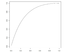
$\boldsymbol{\Lambda}=diag(1,\rho)$

Figure 1: Asymptotic efficiency in $\mathbb{R}^{2}$, as a function of $\rho$, of the eigenprojection of SSCM relative to that of ASSCM.

In three dimensions, $d=3$, the special case we are considering has two sub-cases, namely $\lambda_{2}=\lambda_{3}$ and $\lambda_{1}=\lambda_{2}$, i.e. $(d_{1},d_{2})=(1,2)$ and $(2,1)$ respectively. Presented in Figure 2 are the asymptotic relative efficiencies (18) under both scatter structures as a function of $\rho$. As in two dimensions, the asymptotic relative efficiency is low when $\rho$ is close to 0. Of the two scatter structures considered, the case $(d_{1},d_{2})=(1,2)$ is less favorable for the SSCM.

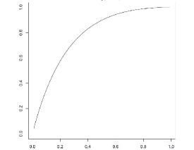
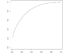
$\boldsymbol{\Lambda}=diag(1,\rho,\rho)$	$\boldsymbol{\Lambda}=diag(1,1,\rho)$

Figure 2: Asymptotic efficiency in $\mathbb{R}^{3}$, as a function of $\rho$, of the eigenprojection of SSCM relative to that of ASSCM.

Plotted in Figure 3 are the asymptotic relative efficiencies when the dimension is $d=5$. The sub-cases here are now $(d_{1},d_{2})=(1,4),(2,3),(3,2)$ and $(4,1)$. From the plots it can be noted that the larger the dimension of the principal component space associated with the larger eigenvalue, the higher the asymptotic relative efficiency, with the asymptotic relative efficiency in the last sub-case not being too low even when $\rho$ approaches zero. This indicates not much is lost by using the SSCM for this case, even under a nearly singular scatter structure. However, as the dimension of the principal component space decreases, the asymptotic relative efficiencies steadily decreases, and can be quite poor for nearly singular scatter structures.

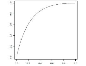
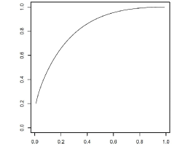
$\boldsymbol{\Lambda}=diag(1,\rho,\rho,\rho,\rho)$	$\boldsymbol{\Lambda}=diag(1,1,\rho,\rho,\rho)$
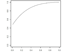
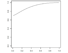
$\boldsymbol{\Lambda}=diag(1,1,1,\rho,\rho)$	$\boldsymbol{\Lambda}=diag(1,1,1,1,\rho)$

Figure 3: Asymptotic efficiency in $\mathbb{R}^{5}$, as a function of $\rho$, of the eigenprojection of SSCM relative to that of ASSCM.

In general, since ${}_{2}F_{1}(a,b;c;0)=1$, the asymptotic relative efficiency (18) goes to one as $\rho\rightarrow 1$. Also, as shown in Appendix 6.3

$$\lim_{\rho\rightarrow 0}ARE_{d,d_{1}}\left(\widehat{\boldsymbol{P}}_{\mathcal{S},1},\widehat{\boldsymbol{P}}_{\mathcal{T},1};\rho\right)=\left\{\begin{array}[]{ccl}\left(1+\frac{2}{d}\right)\left(1-\frac{2}{d_{1}}\right)&\quad\mbox{for}&d_{1}>2\\ 0&\quad\mbox{for}&d_{1}=1,2.\end{array}\right.$$ (20)

A small value of $\rho$ implies the principal component space associated with the larger root is well separated from the principal component space associated with the smaller root. For this case, in high dimensions, for the asymptotic relative efficiency (18) to be greater than $0.80$ or $0.90$, the dimension of the principal component space needs to be at least approximately $d_{1}\geq 10$ and $d_{2}\geq 20$ respectively. Consequently, the SSCM is not particular efficient in cases where principal components analysis is used to reduce the dimensionality of the data to less than ten.

For the scatter structures considered here, to find the asymptotic relative efficiency of the SSCM to an affine equivariant estimate of scatter $\widehat{\boldsymbol{\Gamma}}$ other than Tyler’s scatter matrix, one simply needs to multiply (18) by the asymptotic efficiency of Tyler’s scatter matrix relative to $\widehat{\boldsymbol{\Gamma}}$, which gives $\sigma_{1,\widehat{\boldsymbol{\Gamma}},G}~{}d/(d+2)$. The term $\sigma_{1,\widehat{\boldsymbol{\Gamma}},G}$ is defined as in (4). Note that in contrast to (18), the term $\sigma_{1,\widehat{\boldsymbol{\Gamma}},G}$ does not depend on the values of $\boldsymbol{\Gamma}$ but does depend on the underlying elliptical distribution. Expressions for the $\sigma_{1,\widehat{\boldsymbol{\Gamma}},G}$ for the M-estimates of scatter are given in (Tyler, 1983), and for the high breakdown point S-estimates and re-weighted S-estimates by (Lopuhaä, 1989, 1999). The expressions given for the M-estimates also apply to the high breakdown point MM-estimates. For the sample covariance matrix, $\sigma_{1,\boldsymbol{S}_{n},G}=(1+2/d)E[R_{G}^{4}]/E[R_{G}^{2}]^{2}$, which is one under multivariate normality.

4 Finite Sample Performance

The results of the previous section showed that asymptotically, the inefficiency of the SSCM relative to the ASSCM can be quite severe under an elliptical model which is far from spherical. In this section, the finite sample efficiencies are considered. In the finite sample setting, the behavior of both the SSCM and the ASSCM depend upon the choice of the estimate of location. Also, when estimating location, the finite sample distributions are dependent on the particular elliptical family $\mathcal{E}_{d}(\boldsymbol{\mu},\boldsymbol{\Gamma};G)$, i.e. upon $G$. Here we focus on the estimate based on known $\boldsymbol{\mu}$. For this case, the finite sample distributions of $\widehat{\boldsymbol{\mathcal{S}}}(\boldsymbol{\mu})$ and of $\widehat{\boldsymbol{\mathcal{T}}}(\boldsymbol{\mu})$ do not depend upon $G$. Consequently, for simulation purposes, we only then need to consider random sampling from multivariate normal distributions, even if the true underlying elliptical distribution does not possess any moments. While it is hardly ever the case that the location vector is known a priori, considering this case allows us to focus on the effect of the covariance or scatter structure on the finite sample properties of the estimates.

As in section 3.2, we consider the eigenprojections of the estimates only and do so under the simplified (yet informative) case for which there are just two distinct eigenvalues of multiplicity $d_{1}$ and $d_{2}=d-d_{1}$ respectively. Recall that for this case, the asymptotic variances of the eigenprojections of $\widehat{\boldsymbol{\mathcal{S}}}(\boldsymbol{\mu})$ and $\widehat{\boldsymbol{\mathcal{T}}}(\boldsymbol{\mu})$ under an elliptical distribution are proportional to each other and so the asymptotic comparison of the two estimates is reduced to a single number given by (15). The finite sample variance-covariance matrices of these eigenprojection estimators, however, do not possess the same form as their asymptotic counterparts and are not necessarily proportional to each other. A natural way to compare the eigenprojection estimators to the theoretical eigenprojects is to use the concept of principal (canonical) angles between subspaces.

The notation used in the proceeding paragraphs is consistent with that utilized in Miao & Ben-Israel (1992). Principal angles can be used to describe how far apart one linear subspace is from another. Let $L$ and $M$ be linear subspaces of $\mathbb{R}^{d}$ with $dim\left(L\right)=l\leq dim\left(M\right)=m$. The principal angles between $L$ and $M$, $0\leq\vartheta_{1}\leq\vartheta_{2}\leq\cdots\leq\vartheta_{l}\leq\pi/2$ are given by

$$\hskip 19.91684ptcos\>\vartheta_{i}=\frac{\left\langle{\boldsymbol{x}}_{i},\boldsymbol{y}_{i}\right\rangle}{\|\boldsymbol{x}_{i}\|~{}\|\boldsymbol{y}_{i}\|}=\max\left\{\frac{\left\langle\boldsymbol{x},\boldsymbol{y}\right\rangle}{\left\|\boldsymbol{x}\right\|\left\|\boldsymbol{y}\right\|}:\ \boldsymbol{x}\in L,\ \boldsymbol{x}\perp\boldsymbol{x}_{k},\ \boldsymbol{y}\in M,\ \boldsymbol{y}\perp\textbf{y}_{k},\ k=1,\ldots,i-1\right\},$$ (21)

see e.g. Afriat (1957). If $l=m=1$, then the sole principal angle is simply the smallest angle between two lines. It follows from the above definition that when the two subspaces coincide (i.e. $L=M$) then the principal angles are all $0$. In general, the number of non-zero principal angles is at most $\min(l,d-l)$ with the non-zero princpal angles between $L$ and $M$ being the same as those between $L^{\perp}$ and $M^{\perp}$. The principal angles between two linear subspaces are the maximal invariants under orthogonal transformations of the subspaces. That is, a function $D(L,M)=D(\boldsymbol{Q}L,\boldsymbol{Q}M)$ for any orthogonal transformation $\boldsymbol{Q}$, where $\boldsymbol{Q}L=\{\boldsymbol{x}=\boldsymbol{Q}\boldsymbol{y}:\boldsymbol{y}\in L\}$, if and only if it is a function of the principal angles between $L$ and $M$. The following lemma presents a result given in Björck & Golub (1973) which is useful for computing the principal angles between two linear subspaces.

Lemma 4.1

Let the columns of $Q_{L}\in\mathbb{R}^{n\times l}$ and $Q_{M}\in\mathbb{R}^{n\times m}$ be orthonormal bases for $L$ and $M$ respectively, and let $\sigma_{1}\geq\sigma_{2}\geq\cdots\geq\sigma_{l}\geq 0$ be the singular values of $Q^{T}_{M}Q_{L}$, then $cos\>\vartheta_{i}=\sigma_{i}$ for $i=1,\ldots,l$. Also $\sigma_{l-k}>\sigma_{l-k+1}=\cdots=\sigma_{l}=0$ if and only if $dim\left(L\cap M\right)=k$.

Furthermore, if $\boldsymbol{P}_{L}$ and $\boldsymbol{P}_{M}$ represent the orthogonal projections onto the linear subspaces $L$ and $M$ respectively, then the cosines of the principal angles between $L$ and $M$ correspond to the square roots of the eigenvalues of $\boldsymbol{P}_{L}\boldsymbol{P}_{M}$.

Consider now random samples of size $n$ from an elliptical $\mathcal{E}_{d}(\boldsymbol{\mu},\boldsymbol{\Gamma};G)$ distribution for which $\boldsymbol{\mu}=\boldsymbol{0}$ and for which $\boldsymbol{\Gamma}$ has two distinct eigenvalues with multiplicities $d_{1}$ and $d_{2}=d-d_{1}$. As noted previously, one can assume without loss of generality that the samples come from a multivariate normal distribution $Normal_{d}(\boldsymbol{0},\boldsymbol{\Gamma})$. Furthermore, by orthogonal and scale equivariance, one can also assume without loss of generality that $\boldsymbol{\Gamma}$ is a diagonal matrix with the first $d_{1}$ diagonal elements equal to $\gamma>1$ and the last $d_{2}$ elements equal to $1$, i.e.

$$\boldsymbol{\Gamma}=diag(\underbrace{\gamma,\ldots,\gamma}_{d_{1}},\underbrace{1,\ldots,1}_{d-d_{1}})$$ (22)

The eigenprojection associated with the largest root of $\boldsymbol{\Gamma}$, i.e.  $\boldsymbol{P}_{1}$, then has its upper left $d_{1}\times d_{1}$ block equal to the identity matrix of order $d_{1}$, with all the other blocks equal to zero. The principal angles between the space spanned by an estimated eigenspace, say $\widehat{\boldsymbol{P}}_{1}$, and the space spanned by $\boldsymbol{P}_{1}$ can then be computed by taking the arccosines of the square roots of the eigenvalue of the upper left $d_{1}\times d_{1}$ block of $\widehat{\boldsymbol{P}}_{1}$. For the case $d_{1}=1$, the sole principal angle is then the arcosine of the absolute value of the first element of the normalized eigenvector estimate.

Simulations were undertaken in dimensions $d=2,3$ and $5$ for scatter structures of the form (22). Note that when $d=2$, the only possible case is $d_{1}=1$, for which there is at most one non-zero principal angle. For $d=3$, the two possible cases are $d_{1}=1$ or $d_{1}=2$, for which again there is only one non-zero principal angel. For $d=5$, the cases $d_{1}=1$ or $d_{1}=4$ have at most one non-zero principal angle, whereas the cases $d_{1}=2$ or $d_{1}=3$ have at most two non-zero principal angles. For each of these cases, we consider three situations, namely when the major principal component space explains $90\%$, $95\%$ and 99% of the total variance respectively. In two dimensions with $d_{1}=1$, this corresponds to $\gamma=9,19$ and $99$. In three dimensions, for $d_{1}=1$ the corresponding values of $\gamma=18,38$ and $198$, and for $d_{1}=2$ they are $\gamma=4.5,9.5$ and $49.5$. In five dimensions, for $d_{1}=1$ the corresponding values of $\gamma=36,76,$ and $396$, for $d_{1}=2$ they are $\gamma=13.5,28.5$ and $148.5$, for $d_{1}=3$ they are $6,12.67$ and $66$ and for $d_{1}=4$ they are $\gamma=2.25,4.75$ and $24.75$.

For the ASSCM, due to its affine equivariance, it was only necessary to implement simulations for the case $\boldsymbol{\Gamma}=\boldsymbol{I}_{d}$. For a fixed sample size and dimension, $10,000$ datasets were generated from a $Normal_{d}(\boldsymbol{0},\boldsymbol{I}_{d})$ distribution. The ASSCM, $\widehat{\boldsymbol{\mathcal{T}}}_{n}$, was calculated for each dataset. By affine equivariance, the ASSCM matrices for other scatter structures were obtained by transforming $\widehat{\boldsymbol{\mathcal{T}}}_{n}\rightarrow\boldsymbol{\Gamma}^{1/2}\widehat{\boldsymbol{\mathcal{T}}}_{n}\boldsymbol{\Gamma}^{1/2}$. For the SSCM, since it is only scale and orthogonally equivariant, it was necessary to implement simulations for each sample size, dimension and scatter structure considered. For each case considered, $10,000$ datasets were generated and the SSCM, $\widehat{\boldsymbol{\mathcal{S}}}_{n}$, was calculated for each dataset. The principal angles between $\widehat{\boldsymbol{P}}_{\mathcal{T},1}$ and $\boldsymbol{P}_{1}$, as well as the principal angles between $\widehat{\boldsymbol{P}}_{\mathcal{S},1}$ and $\boldsymbol{P}_{1}$, were then calculated as previously described. Denote the principal angles between $\widehat{\boldsymbol{P}}_{\mathcal{T},1}$ and $\boldsymbol{P}_{1}$ by $\widehat{\tau}_{1}\geq\ldots\geq\widehat{\tau}_{d_{1}}\geq 0$ and the principal angles between $\widehat{\boldsymbol{P}}_{\mathcal{S},1}$ and $\boldsymbol{P}_{1}$ by $\widehat{\omega}_{1}\geq\ldots\geq\widehat{\omega}_{d_{1}}\geq 0$. Since large deviations of the principal angles from zero indicate a poor estimate, the sum of the squared principal angles gives a measure of loss of an eigenprojection estimate. A measure of relative efficiency of $\widehat{\boldsymbol{P}}_{\mathcal{S},1}$ to $\widehat{\boldsymbol{P}}_{\mathcal{T},1}$ can then be obtained by comparing the size of $T_{n}=\widehat{\tau}_{1}^{2}+\cdots+\widehat{\tau}_{d_{1}}^{2}$ to that of $\Omega_{n}=\widehat{\omega}_{1}^{2}+\cdots+\widehat{\omega}_{d_{1}}^{2}$ using some measure of central tendency. Here, we consider both the expected value and the median and so define the following two measures of finite sample relative efficiency

$$RE_{1,n}\left[\widehat{\boldsymbol{P}}_{\mathcal{S},1},\widehat{\boldsymbol{P}}_{\mathcal{T},1};\boldsymbol{\Gamma}\right]=\frac{E\left[T_{n}\right]}{E\left[\Omega_{n}\right]}\quad\mbox{and}\quad RE_{2,n}\left[\widehat{\boldsymbol{P}}_{\mathcal{S},1},\widehat{\boldsymbol{P}}_{\mathcal{T},1};\boldsymbol{\Gamma}\right]=\frac{median\left[T_{n}\right]}{median\left[\Omega_{n}\right]}$$ (23)

We show in Appendix 6.4 that the limiting value of $RE_{2,n}$ is equal to the asymptotic relative efficiency given by (15), where here $\rho^{2}=\lambda_{(2)}/\lambda_{(1)}=1/\gamma$, and we conjecture that this also holds for $RE_{1,n}$.

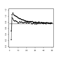
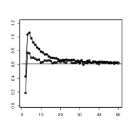
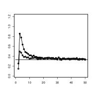
$d_{1}=1,\gamma=9.0$	$d_{1}=1,\gamma=19.0$	$d_{1}=1,\gamma=99.0$

Figure 4: Finite sample relative efficiencies in $\mathbb{R}^{2}$ for the scatter structure (22), as a function of sample size, of the eigenprojection of the SSCM to that of the ASSCM. Black and grey circles refer to $RE_{1,n}$ and $RE_{2,n}$, (23) respectively.

Figures 4, 5, and 6 show the simulated values of the relative efficiencies (23) for dimensions $d=2,3$ and $5$ respectively. For $d=2$ and $3$, the sample sizes are $n=d,\ldots,50$. When $d=5$, the simulations were done for sample sizes $n=5,10,\ldots,125$. In all of the figures, it can be observed that the finite sample relative efficiency quickly decreases to the asymptotic relative efficiency, which is indicated by the horizontal line. For smaller sample sizes, the finite sample relative efficiency using the median based measure, $RE_{2,n}$, is considerably smaller than that using the expected value based measure, $RE_{1,n}$. Also, for relatively small samples sizes, the deficiency of the SSCM is not as pronounced as in larger sample sizes. The one exception to this trend is when $n=d$. For this case, it is known that the ASCCM or Tyler’s matrix is proportional to the sample covariance matrix, and that the sample covariance matrix is proportional to the maximum likelihood estimate for the shape matrix $\boldsymbol{\Gamma}$ not only under the multivariate normal model but also under any elliptical model, see (Tyler, 2010).

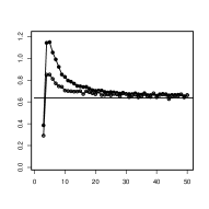
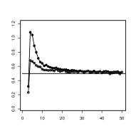
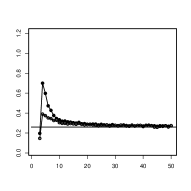
$d_{1}=1,\gamma=18.0$	$d_{1}=1,\gamma=38.0$	$d_{1}=1,\gamma=198.0$
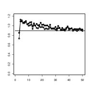
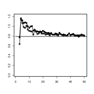
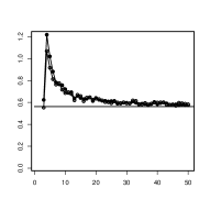
$d_{1}=2,\gamma=4.5$	$d_{1}=2,\gamma=9.5$	$d_{1}=2,\gamma=49.5$

Figure 5: Finite sample relative efficiencies in $\mathbb{R}^{3}$ for the scatter structure (22), as a function of sample size, of the eigenprojection of the SSCM to that of the ASSCM. Black and grey circles refer to $RE_{1,n}$ and $RE_{2,n}$, (23) respectively.

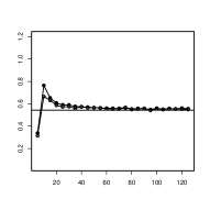
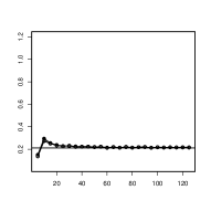
$d_{1}=1,\gamma=36.0$	$d_{1}=1,\gamma=76.0$	$d_{1}=1,\gamma=396.0$
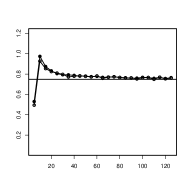
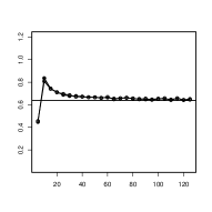
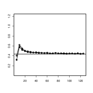
$d_{1}=2,\gamma=13.5$	$d_{1}=2,\gamma=28.5$	$d_{1}=2,\gamma=148.5$
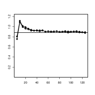
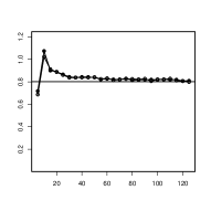
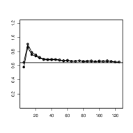
$d_{1}=3,\gamma=6.0$	$d_{1}=3,\gamma=12.67$	$d_{1}=3,\gamma=66.0$
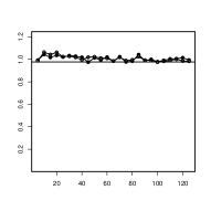
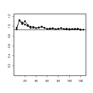
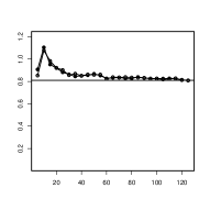
$d_{1}=4,\gamma=2.25$	$d_{1}=4,\gamma=4.75$	$d_{1}=4,\gamma=24.75$

Figure 6: Finite sample relative efficiencies in $\mathbb{R}^{5}$ for the scatter structure (22), as a function of sample size, of the eigenprojection of the SSCM to that of the ASSCM. Black and grey circles refer to $RE_{1,n}$ and $RE_{2,n}$, (23) respectively.

5 Concluding Remarks

The spatial sign covariance matrix (SSCM) has been proposed in the past as an alternative estimate of scatter/shape based on its robustness properties and computational simplicity. These benefits, though, do not arise without a cost. For the case when the data arises from an elliptically symmetric distribution, it is known that in general the SSCM is a biased estimate of shape parameter $\boldsymbol{\Gamma}$, and in particular the eigenvalues of the SSCM are biased estimates of the eigenvalues of $\boldsymbol{\Gamma}$. However, as a consequence of the SSCM being orthogonally equivariant, the corresponding eigenvectors, or more generally eigenprojections, of the SSCM are unbiased estimates of the eigenvectors/eigenprojections of $\boldsymbol{\Gamma}$. Due to its robustness, computational simplicity and orthogonal equivariance, the SSCM has been suggested for extracting principal components vectors, which is an orthogonally equivariant procedure. However, this paper demonstrates that under the elliptical model, even the estimates of eigenvectors/eigenprojections based on the SSCM are affected by the lack of affine equivariance of the SSCM and are highly inefficient in situations for which PCA is of most interest.

In the current paper it is proven that a consistency adjusted SSCM (obtain by replacing the eigenvalues of the SSCM estimate with unbiased ones) is asymptotically inadmissible when compared to a well studied affine equivariant version of the SSCM, Tyler’s estimate of scatter, which is referred to in the paper as the ASSCM. The asymptotic relative efficiency of an eigenprojection based on the SSCM relative to that based on the ASSCM is shown to be quit severe, in particular for nearly singular scatter structures when the dimension of the principal component space with the highest variability is small compared to the dimension of the data. This situation is when PCA is of most value as a dimension reduction method. Finite sample simulations were implemented which also demonstrate the inefficiency of the eigenprojection estimates based on the SSCM for relatively small sample sizes. It should be noted that the current paper can be considered as complementary to Magyar & Tyler (2012) in which the inefficiency of the spatial median, a popular orthogonally equivariant estimate of location was studied in detail under the elliptical model.

As noted at the end of section 3.2, the asymptotic efficiency of the SSCM relative to any affine equaivariant estimate can be obtain by making a simple scalar adjustment, not dependent on $\boldsymbol{\Gamma}$, to the asymptotic relative efficiency of the SSCM to the ASSCM. The main advantage of the SSCM over a high breakdown point affine equivariant scatter estimate is its computational simplicity. The main advantage of the SSCM over computationally simple affine equivariant scatter estimates, such as the M-estimates of scatter, is its higher breakdown point. The SSCM has a breakdown point of $1/2$, whereas the M-estimates of scatter have breakdown points at best $1/d$, with Tyler’s estimate of scatter acheiving a breakdown point of $1/2$, see e.g. Dümbgen & Tyler (2005) who also show that the breakdown of the M-estimates occur only under very specific types of contamination. It is also worth noting, as argued in Davies & Gather (2005), that the concept of the breakdown point of a scatter matrix is not as meaningful outside of the affine equivariant setting. For example, the sample covariance matrix $\boldsymbol{S}_{n}$ can be easily adjusted to have breakdown point $1/2$ by expressing it in terms of it spectral value decomposition $\boldsymbol{S}_{n}=\boldsymbol{Q}_{n}\boldsymbol{\Delta}_{n}\boldsymbol{Q}_{n}^{T}$ and then defining $\boldsymbol{S}_{n}^{*}=\boldsymbol{Q}_{n}\boldsymbol{\Delta}^{*}_{n}\boldsymbol{Q}_{n}^{T}$, where $\boldsymbol{\Delta}^{*}_{n}$ is a diagonal matrix consisting of the squares of the marginal median absolute deviations of $\boldsymbol{Q}_{n}^{T}\boldsymbol{x}_{i}$. Note that $\boldsymbol{S}_{n}$ and $\boldsymbol{S}^{*}_{n}$ have the same eigenvectors, but that $\boldsymbol{S}^{*}_{n}$ is only orthogonally equivariant and has breakdown point $1/2$. Finally, it should be noted that for affine equivariant scatter estimates the concept of the breakdown point and the breakdown point at the edge are equivalent, but this is not the case for non-affine equivariant scatter statistics, see Stahel (1981); Hampel et al. (1986). The breakdown point at the edge of a scatter statistic is the multivariate equivalent of the exact fit property in regression. It roughly corresponds to the proportion of contamination one needs to add to a lower dimensional data set in order for the scatter statistics to become non-singular. If the scatter statistic is not affine equivariant, then the breakdown at the edge is known to be zero, again see Stahel (1981); Hampel et al. (1986). This again suggest that the SSCM is not particularly robust when the underlying scatter structure is nearly singular.

6 Appendix

6.1 Review of some matrix algebra

The notation used within the paper has become fairly standard and is as follows. If $\boldsymbol{A}$ is a $p\times q$ matrix, then $vec(\boldsymbol{A})$ is the $pq$-dimensional vector formed by stacking the columns of $\boldsymbol{A}$. If $\boldsymbol{A}$ is a $p\times q$ matrix and $B$ is a $r\times s$ matrix, then the Kronecker product of $A$ and $B$ is the $pr\times qs$ partitioned matrix $\boldsymbol{A}\otimes\boldsymbol{B}=[a_{jk}\boldsymbol{B}]$. The commutation matrix $\mathcal{K}_{a,b}$ is the $ab\times ab$ matrix $\sum_{i=1}^{a}\sum_{j=1}^{b}\boldsymbol{J}_{ij}\otimes\boldsymbol{J}^{T}_{ij}$, where $\boldsymbol{J}_{ij}$ is an $a\times b$ matrix with a one in the $(i,j)$ position and zeros elsewhere. Algebraic properties involving the $vec$ transformation, the Kronecker product and the commutation matrix can be found e.g. in Bilodeau & Brenner (1999). Some important properties, which are to be used without further reference, are:

$$\begin{array}[]{ccc}vec(\boldsymbol{A}\boldsymbol{B}\boldsymbol{C})=(\boldsymbol{C}^{T}\otimes\boldsymbol{A})vec(\boldsymbol{B}),&\quad\mathcal{K}_{d,d}^{2}=\boldsymbol{I}_{d^{2}},&(\boldsymbol{A}\otimes\boldsymbol{B})(\boldsymbol{C}\otimes\boldsymbol{D})=(\boldsymbol{A}\boldsymbol{C}\otimes\boldsymbol{B}\boldsymbol{D}),\\[6.0pt] \mathcal{K}_{r,p}(\boldsymbol{A}\otimes\boldsymbol{B})=(\boldsymbol{B}\otimes\boldsymbol{A})\mathcal{K}_{s,q},&\quad\mbox{and}&\mathcal{K}_{p,q}vec(\boldsymbol{A})=vec(\boldsymbol{A}^{T}).\end{array}$$ (24)

6.2 Asymptotic Distribution of Eigenprojections of a Scatter Estimate

The proof of equation (12) is given in this section. To begin, results for the asymptotic distribution for eigenprojections in general given in Tyler (1981) are partially reviewed and extended here. Let $\boldsymbol{M}$ be a $d\times d$ positive definite symmetric matrix with eigenvalues $\eta_{(1)}>\eta_{(2)}>\cdots>\eta_{(m)}$ having multiplicities $d_{1},\ldots,d_{m}$ respectively, and corresponding eigenprojections $\boldsymbol{P}_{1},\ldots,\boldsymbol{P}_{m}$. Suppose $\boldsymbol{M}_{n}$ is a sequence of random positive definite symmetric matrices such that $\sqrt{n}(\boldsymbol{M}_{n}-\boldsymbol{M})\rightarrow_{\mathcal{D}}\boldsymbol{N}$, with $vec(\boldsymbol{N})$ having a $Normal_{d^{2}}(\boldsymbol{0},\boldsymbol{\mathcal{V}}_{\boldsymbol{M}})$ distribution. Similar to the definitions of $\widehat{\boldsymbol{P}}_{\mathcal{T},j}$ and $\widehat{\boldsymbol{P}}_{\mathcal{S},j}$, let $\widehat{\boldsymbol{P}}_{j}$ denote the consistent estimate of $\boldsymbol{P}_{j}$. It then follows from Theorem 4.1 in Tyler (1981) that

$$\sqrt{n}(\widehat{\boldsymbol{P}}_{j}-\boldsymbol{P}_{j})\rightarrow_{\mathcal{D}}\boldsymbol{P}_{j}\boldsymbol{N}(\boldsymbol{M}-\eta_{(j)}\boldsymbol{I}_{d})^{+}+(\boldsymbol{M}-\eta_{(j)}\boldsymbol{I}_{d})^{+}\boldsymbol{N}\boldsymbol{P}_{j},$$

where $\boldsymbol{A}^{+}$ denotes the Moore-Penrose generalized inverse of $\boldsymbol{A}$. Using the properties given in (24), and noting that $vec\{\boldsymbol{N}\}=vec\{\boldsymbol{N}^{T}\}=\mathcal{K}_{d,d}vec\{\boldsymbol{N}\}$, one obtains

$$\sqrt{n}~{}vec\left\{\widehat{\boldsymbol{P}}_{j}-\boldsymbol{P}_{j}\right\}\rightarrow_{\mathcal{D}}\left(\boldsymbol{I}_{d^{2}}+\mathcal{K}_{d,d}\right)\left\{\boldsymbol{P}_{j}\otimes\left(\boldsymbol{M}-\eta_{(j)}\boldsymbol{I}_{d}\right)^{+}vec\{\boldsymbol{N}\}\right\},$$

and hence $\sqrt{n}~{}vec\left\{\widehat{\boldsymbol{P}}_{j}-\boldsymbol{P}_{j}\right\}\rightarrow_{\mathcal{D}}Normal_{d^{2}}\left(\boldsymbol{0},\boldsymbol{\mathcal{V}}_{\boldsymbol{P}_{j}}\right)$ where

$$\boldsymbol{\mathcal{V}}_{\boldsymbol{P}_{j}}=\left(\boldsymbol{I}_{d^{2}}+\mathcal{K}_{d,d}\right)\left\{\boldsymbol{P}_{j}\otimes\left(\boldsymbol{M}-\eta_{(j)}\boldsymbol{I}_{d}\right)^{+}\right\}\boldsymbol{\mathcal{V}}_{\boldsymbol{M}}\left\{\boldsymbol{P}_{j}\otimes\left(\boldsymbol{M}-\eta_{(j)}\boldsymbol{I}_{d}\right)^{+}\right\}\left(\boldsymbol{I}_{d^{2}}+\mathcal{K}_{d,d}\right)$$ (25)

Suppose now that $\boldsymbol{\mathcal{V}}_{\boldsymbol{M}}$ is of the form

$$\boldsymbol{\mathcal{V}}_{\boldsymbol{M}}=\sigma_{1}(\boldsymbol{I}_{d^{2}}+\mathcal{K}_{d,d})(\boldsymbol{M}\otimes\boldsymbol{M})+\sigma_{2}vec\{\boldsymbol{M}\}vec\{\boldsymbol{M}\}^{T},$$ (26)

as is the case when $\boldsymbol{M}_{n}$ is an affine equivariant scatter estimate based on a random sample from an elliptical distribution, see Tyler (1983), then (25) becomes

$$\boldsymbol{\mathcal{V}}_{\boldsymbol{P}_{j}}=\sigma_{1}\left(\boldsymbol{I}_{d^{2}}+\mathcal{K}_{d,d}\right)\sum_{k=1,k\neq j}^{m}\frac{\eta_{(j)}\eta_{(k)}}{(\eta_{(k)}-\eta_{(j)})^{2}}(\boldsymbol{P}_{j}\otimes\boldsymbol{P}_{k}+\boldsymbol{P}_{k}\otimes\boldsymbol{P}_{j}).$$ (27)

To verify this last result note that $\boldsymbol{M}\boldsymbol{P}_{j}=\eta_{(j)}\boldsymbol{P}_{j}$, $\boldsymbol{P}_{j}\boldsymbol{P}_{j}=\boldsymbol{P}_{j}$, and for $k\neq j$, $\boldsymbol{P}_{j}\boldsymbol{P}_{k}=\boldsymbol{0}$. So, for $k\neq j$, $(\boldsymbol{P}_{j}\otimes\boldsymbol{P}_{k})vec(\boldsymbol{M})=vec\left\{\boldsymbol{P}_{k}\boldsymbol{M}\boldsymbol{P}_{j}\right\}=\boldsymbol{0}$, $(\boldsymbol{P}_{j}\otimes\boldsymbol{P}_{k})(\boldsymbol{M}\otimes\boldsymbol{M})(\boldsymbol{P}_{j}\otimes\boldsymbol{P}_{k})=\eta_{(j)}\eta_{(k)}(\boldsymbol{P}_{j}\otimes\boldsymbol{P}_{k})$, and ($\boldsymbol{P}_{j}\otimes\boldsymbol{P}_{k})\mathcal{K}_{d,d}(\boldsymbol{M}\otimes\boldsymbol{M})(\boldsymbol{P}_{j}\otimes\boldsymbol{P}_{k})=\mathcal{K}_{d,d}(\boldsymbol{P}_{k}\otimes\boldsymbol{P}_{j})(\boldsymbol{M}\otimes\boldsymbol{M})(\boldsymbol{P}_{j}\otimes\boldsymbol{P}_{k})=\boldsymbol{0}.$ Hence,

$$\ \left(\boldsymbol{I}_{d^{2}}+\mathcal{K}_{d,d}\right)(\boldsymbol{P}_{j}\otimes\boldsymbol{P}_{k})\boldsymbol{\mathcal{V}}_{\boldsymbol{M}}(\boldsymbol{P}_{j}\otimes\boldsymbol{P}_{k})\left(\boldsymbol{I}_{d^{2}}+\mathcal{K}_{d,d}\right)=\sigma_{1}\eta_{(j)}\eta_{(j)}\left(\boldsymbol{I}_{d^{2}}+\mathcal{K}_{d,d}\right)(\boldsymbol{P}_{j}\otimes\boldsymbol{P}_{k})\left(\boldsymbol{I}_{d^{2}}+\mathcal{K}_{d,d}\right).$$

Also, $\left(\boldsymbol{I}_{d^{2}}+\mathcal{K}_{d,d}\right)(\boldsymbol{P}_{j}\otimes\boldsymbol{P}_{k})\left(\boldsymbol{I}_{d^{2}}+\mathcal{K}_{d,d}\right)=\left(\boldsymbol{I}_{d^{2}}+\mathcal{K}_{d,d}\right)(\boldsymbol{P}_{j}\otimes\boldsymbol{P}_{k}+\boldsymbol{P}_{j}\otimes\boldsymbol{P}_{k})$, and for distinct $j,k,k^{\prime}$, $(\boldsymbol{P}_{j}\otimes\boldsymbol{P}_{k})\boldsymbol{\mathcal{V}}_{\boldsymbol{M}}(\boldsymbol{P}_{j}\otimes\boldsymbol{P}_{k^{\prime}})=\boldsymbol{0}$. Expression (27) then follows by using the spectral representation $\left(\boldsymbol{M}-\eta_{(j)}\boldsymbol{I}_{d}\right)^{+}=\sum_{k\neq j}(\eta_{(k)}-\eta_{(j)})^{-1}\boldsymbol{P}_{k}$.

For Tyler’s scatter estimate, the eigenprojections for $\widehat{\boldsymbol{\mathcal{T}}}_{n}$ and for $\widehat{\boldsymbol{\mathcal{T}}}_{o,n}=\left(d/\mbox{trace}\{\boldsymbol{\Gamma}^{-1}\widehat{\boldsymbol{\mathcal{T}}}_{n}\}\right)\widehat{\boldsymbol{\mathcal{T}}}_{n}$ are the same, namely$\widehat{\boldsymbol{P}}_{\mathcal{T},j}$. Under any elliptical distribution, the asymptotic variance for $\widehat{\boldsymbol{\mathcal{T}}}_{o,n}$ is shown in Tyler (1987a) to have the form (26) with $\sigma_{1}=(d+2)/d$, $\sigma_{2}=2/d$ and with $\boldsymbol{M}=\boldsymbol{\Gamma}$. Equation (27) thus applies, and this establishes (12) for the case $\boldsymbol{\mathcal{V}}_{\mathcal{T},j}(\boldsymbol{\Gamma})$.

The result (12) for $\boldsymbol{\mathcal{V}}_{\mathcal{S},j}(\boldsymbol{\Gamma})$ is more complicated to establish since the SSCM is not affine equivariant. Using the spectral value decomposition $\boldsymbol{\Gamma}=\boldsymbol{Q}\boldsymbol{\Lambda}\boldsymbol{Q}^{T}$, it follows that $\boldsymbol{\mathcal{V}}_{\mathcal{S},j}(\boldsymbol{\Gamma})=(\boldsymbol{Q}\otimes\boldsymbol{Q})\boldsymbol{\mathcal{V}}_{\mathcal{S},j}(\boldsymbol{\Lambda})(\boldsymbol{Q}\otimes\boldsymbol{Q})^{T}$, and so it is sufficient to consider the the special case $\boldsymbol{\Gamma}=\boldsymbol{\Lambda}=diagonal(\lambda_{1},\ldots,\lambda_{d})$. The asymptotic variance of $\widehat{\boldsymbol{\mathcal{S}}}_{n}$ is then given by $\boldsymbol{\mathcal{V}}_{\mathcal{S}}=var\left(vec\{\boldsymbol{\theta}\boldsymbol{\theta}^{T}\}\right)=E[\boldsymbol{\theta}\boldsymbol{\theta}^{T}\otimes\boldsymbol{\theta}\boldsymbol{\theta}^{T}]-vec(\boldsymbol{\Delta})vec(\boldsymbol{\Delta})^{T}$, where $\boldsymbol{\theta}=\sim_{\mathcal{D}}ACG_{d}(\boldsymbol{\Lambda})$. We proceed by first finding an expression for $E[\boldsymbol{\theta}\boldsymbol{\theta}^{T}\otimes\boldsymbol{\theta}\boldsymbol{\theta}^{T}]$.

Let $\boldsymbol{e}_{1},\ldots\boldsymbol{e}_{d}$ represent the Euclidean bases elements in $\mathbb{R}^{d}$, then

$$E[\boldsymbol{\theta}\boldsymbol{\theta}^{T}\otimes\boldsymbol{\theta}\boldsymbol{\theta}^{T}]=\sum_{p=1}^{d}\sum_{q=1}^{d}\sum_{r=1}^{d}\sum_{s=1}^{d}a_{pqrs}(\boldsymbol{e}_{p}\boldsymbol{e}_{q}^{T}\otimes\boldsymbol{e}_{r}\boldsymbol{e}_{s}^{T}),$$

where $a_{pqrs}=E[\theta_{p}\theta_{q}\theta_{r}\theta_{s}]$. Since $\boldsymbol{\theta}$ is symmetrically distributed in each coordinate, it follows that $a_{pqrs}=0$ unless $p=q=r=s$, $p=q$ and $r=s$, $p=r$ and $q=s$, or $p=s$ and $q=r$. Also, since $(\boldsymbol{e}_{p}\boldsymbol{e}_{q}^{T}\otimes\boldsymbol{e}_{q}\boldsymbol{e}_{p}^{T})=\mathcal{K}_{d,d}(\boldsymbol{e}_{p}\boldsymbol{e}_{p}^{T}\otimes\boldsymbol{e}_{q}\boldsymbol{e}_{q}^{T})$, $E[\boldsymbol{\theta}\boldsymbol{\theta}^{T}\otimes\boldsymbol{\theta}\boldsymbol{\theta}^{T}]$ can be expressed as

$$(\boldsymbol{I}_{d^{2}}+\mathcal{K}_{d,d})\left(\sum_{p=1}^{d}\sum_{q=1}^{d}\gamma_{pq}(\boldsymbol{e}_{p}\boldsymbol{e}_{p}^{T}\otimes\boldsymbol{e}_{q}\boldsymbol{e}_{q}^{T})-\sum_{p=1}^{d}\gamma_{pp}(\boldsymbol{e}_{p}\boldsymbol{e}_{p}^{T}\otimes\boldsymbol{e}_{p}\boldsymbol{e}_{p}^{T})\right)+\sum_{p=1}^{d}\sum_{q=1}^{d}\gamma_{pq}(\boldsymbol{e}_{p}\boldsymbol{e}_{q}^{T}\otimes\boldsymbol{e}_{p}\boldsymbol{e}_{q}^{T}),$$

where $\gamma_{pq}=E[\theta_{p}^{2}\theta_{q}^{2}]$.

Equation (25) can now be applied to $\widehat{\boldsymbol{P}}_{\mathcal{S},j}$ with $\boldsymbol{M}=\boldsymbol{\Xi}=\boldsymbol{\Delta}=diagonal(\phi_{1},\ldots\phi_{d})$ and $\boldsymbol{P}_{j}=\boldsymbol{E}_{j}=\sum_{i=m_{j}+1}^{m_{j}+d_{j}}\boldsymbol{e}_{i}\boldsymbol{e}_{i}^{T}$. The term $\left\{\boldsymbol{E}_{j}\otimes\left(\boldsymbol{\Delta}-\phi_{(j)}\right)^{+}\right\}vec(\boldsymbol{\Delta})=vec(\left(\boldsymbol{\Delta}-\phi_{(j)}\right)^{+}\boldsymbol{\Delta}\boldsymbol{E}_{j})=\boldsymbol{0}$, and for $p\neq q$, $\left\{\boldsymbol{E}_{j}\otimes\left(\boldsymbol{\Delta}-\phi_{(j)}\boldsymbol{I}_{d}\right)^{+}\right\}(\boldsymbol{e}_{p}\boldsymbol{e}_{q}^{T}\otimes\boldsymbol{e}_{p}\boldsymbol{e}_{q}^{T})\left\{\boldsymbol{E}_{j}\otimes\left(\boldsymbol{\Delta}-\phi_{(j)}\boldsymbol{I}_{d}\right)^{+}\right\}=\boldsymbol{0}$. Furthermore, using the fourth property in (24), it follows that $\left\{\boldsymbol{E}_{j}\otimes\left(\boldsymbol{\Delta}-\phi_{(j)}\boldsymbol{I}_{d}\right)^{+}\right\}\mathcal{K}_{d,d}(\boldsymbol{e}_{p}\boldsymbol{e}_{p}^{T}\otimes\boldsymbol{e}_{q}\boldsymbol{e}_{q}^{T})\left\{\boldsymbol{E}_{j}\otimes\left(\boldsymbol{\Delta}-\phi_{(j)}\boldsymbol{I}_{d}\right)^{+}\right\}=\boldsymbol{0}.$ Hence, $\boldsymbol{\mathcal{V}}_{\boldsymbol{M}}=\boldsymbol{\mathcal{V}}_{\mathcal{S}}$ in (25) can be replaced by $\sum_{p=1}^{d}\sum_{q=1}^{d}\gamma_{pq}(\boldsymbol{e}_{p}\boldsymbol{e}_{p}^{T}\otimes\boldsymbol{e}_{q}\boldsymbol{e}_{q}^{T}).$

Next, observe that the term

$$\left\{\boldsymbol{E}_{j}\otimes\left(\boldsymbol{\Delta}-\phi_{(j)}\boldsymbol{I}_{d}\right)^{+}\right\}(\boldsymbol{e}_{p}\boldsymbol{e}_{p}^{T}\otimes\boldsymbol{e}_{q}\boldsymbol{e}_{q}^{T})\left\{\boldsymbol{E}_{j}\otimes\left(\boldsymbol{\Delta}-\phi_{(j)}\boldsymbol{I}_{d}\right)^{+}\right\}=\left(\phi_{q}-\phi_{(j)}\right)^{-2}(\boldsymbol{e}_{p}\boldsymbol{e}_{p}^{T}\otimes\boldsymbol{e}_{q}\boldsymbol{e}_{q}^{T}),$$

for $p\in\{m_{j}+1,\ldots,m_{j}+d_{j}\}$ and $q\not\in\{m_{j}+1,\ldots,m_{j}+d_{j}\}$, and is $\boldsymbol{0}$ otherwise. Also, the value of $\gamma_{pq}$ is the same for all $p\in\{m_{j}+1,\ldots,m_{j}+d_{j}\}$ and $q\in\{m_{k}+1,\ldots,m_{k}+d_{k}\}$, say $\psi_{(j,k)}$. Hence,

$$\boldsymbol{\mathcal{V}}_{\mathcal{S},j}(\boldsymbol{\Lambda})=(\boldsymbol{I}_{d^{2}}+\mathcal{K}_{d,d})\left\{\sum_{k=1,k\neq j}^{m}\frac{\psi_{(j,k)}}{\left(\phi_{q}-\phi_{(j)}\right)^{2}}(\boldsymbol{E}_{j}\otimes\boldsymbol{E}_{k})\right\}(\boldsymbol{I}_{d^{2}}+\mathcal{K}_{d,d}).$$

This can be seen to agree with (12) for the special case $\boldsymbol{\Gamma}=\boldsymbol{\Lambda}$ after again noting that

$$(\boldsymbol{I}_{d^{2}}+\mathcal{K}_{d,d})(\boldsymbol{E}_{j}\otimes\boldsymbol{E}_{k})(\boldsymbol{I}_{d^{2}}+\mathcal{K}_{d,d})=(\boldsymbol{I}_{D^{2}}+\mathcal{K}_{d,d})(\boldsymbol{E}_{j}\otimes\boldsymbol{E}_{k}+\boldsymbol{E}_{k}\otimes\boldsymbol{E}_{j}).$$

The form for $\psi_{(j,k)}$ given in (12) is obtained by noting $\theta_{p}^{2}\sim_{\mathcal{D}}\lambda_{p}\chi^{2}_{1,p}/\sum_{q=1}^{d}\lambda_{q}\chi^{2}_{1,q}$ with $\chi^{2}_{1,i}$, for $i=1,\ldots,d$ having independent chi-square distributions on one degree of freedom, and

$$\psi_{(j,k)}=(d_{j}d_{k})^{-1}\sum_{p=m_{j}+1}^{m_{j}+d_{j}}\sum_{q=m_{k}+1}^{m_{k}+d_{k}}\gamma_{pg}.$$

6.3 The Gauss Hypergeometric Functions.

Proof of statements (16) and (17). The expressions for $\psi_{(1,2)}$ and $\phi_{(i)},i=1,2$ arise from the following two observations. First, $U=\chi^{2}_{(2)}/\left(\chi^{2}_{(1)}+\chi^{2}_{(2)}\right)\sim_{\mathcal{D}}Beta\left(\frac{d_{2}}{2},\frac{d_{1}}{2}\right)$, and second ${}_{2}F_{1}\left(a,b;c;k\right)=B^{-1}\left(b,c-b\right)\int^{1}_{0}x^{b-1}\left(1-x\right)^{c-b-1}\left(1-kx\right)^{-a}dx$, where $B\left(a,b\right)=\Gamma\left(a\right)\Gamma\left(b\right)/\Gamma\left(a+b\right)$ is the Beta function, see e.g. (15.2.1) in Abramowitz & Stegun (1992). The integral representation of the Gauss hypergeometric function is valid for $\Re\left(c\right)>\Re\left(b\right)>0$. From this, evaluation of the following expectation is straightforward,

$$E\left[U^{r}\left(1-U\right)^{s}\left(1-\kappa U\right)^{-t}\right]=\frac{B\left(\frac{d_{2}+2r}{2},\frac{d_{1}+2s}{2}\right)}{B\left(\frac{d-d_{1}}{2},\frac{d_{1}}{2}\right)}~{}{}_{2}F_{1}\left(t,\frac{d-d_{1}+2r}{2};\frac{d+2s+2r}{2};\kappa\right).$$

Expressions (16) and (17) then follow since, for $\kappa=1-\rho^{2}$,

$$\psi_{(1,2)}=\frac{\rho^{2}}{d_{1}d_{2}}E\left[\frac{U(1-U)}{\left(1-\kappa U\right)^{2}}\right],\quad\phi_{(1)}=\frac{1}{d_{1}}E\left[\frac{1-U}{1-\kappa U}\right]\quad\mbox{and}\quad\phi_{(2)}=\frac{\rho^{2}}{d_{2}}E\left[\frac{U}{1-\kappa U}\right].$$

More details on the above derivations and on the following derivations can be found in the dissertation by Magyar (2012).

Proof of statement (18). The form for the asymptotic relative efficiency can be obtained by inserting (16) and (17) into the expressions for $\alpha_{\mathcal{T}}(\rho)$ and $\alpha_{\mathcal{S}}(\rho)$ given in (13), and then simplifying the ratio $\alpha_{\mathcal{T}}(\rho)/\alpha_{\mathcal{S}}(\rho)$ using the identity (15.2.20) in Abramowitz & Stegun (1992), i.e.

$$\frac{1-\kappa}{\kappa}\,_{2}F_{1}\left(a,b;c;\kappa\right)-\frac{1}{\kappa}\,_{2}F_{1}\left(a-1,b;c;\kappa\right)+\frac{c-b}{c}\,_{2}F_{1}\left(a,b;c+1;\kappa\right)=0,$$

with $a=(d_{2}+2)/2,b=1$, and $c=(d+2)/2$.

Proof of statement (19). The form for $\phi_{(2)}$ can be obtained by using the identity (15.1.14) in Abramowitz & Stegun (1992), namely ${}_{2}F_{1}\left(a,\frac{1}{2}+a;2a;\kappa\right)=2^{2a-1}\left[1+(1-\kappa)^{1/2}\right]^{1-2a}$ with $a=1$. The form for $\phi_{(1)}$ then follows since $\phi_{(1)}+\phi_{(2)}=1$. Finally, the form for $\psi_{(1,2)}$ follows from identity $(1-\kappa)^{1/2}~{}{}_{2}F_{1}\left(1+a,\frac{1}{2}+a;1+2a;\kappa\right)=2^{2a}\left[1+(1-\kappa)^{1/2}\right]^{-2a}$ using $a=1$, see (15.1.13) in Abramowitz & Stegun (1992).

Proof of statement (20). Identity (15.1.20) in Abramowitz & Stegun (1992) states ${}_{2}F_{1}\left(a,b;c;1)\right)=\{\Gamma(c)\Gamma(c-a-b)\}/\{\Gamma(c-a)\Gamma(c-b)\}$ provided $c>a+b$. Taking the limit as $\rho\rightarrow 0$ in (18) and applying this identity gives (20) for the case $d_{1}>2$. The cases $d_{1}=1,2$ require special treatment since for these cases $c-a-b=(d_{1}-2)/2\leq 0$. Here the the identity (15.3.3) in Abramowitz & Stegun (1992) is useful. This states that ${}_{2}F_{1}(a;b;c;\kappa)=(1-\kappa)^{c-a-b}{}_{2}F_{1}(c-a;c-b;c;\kappa)$. From this it follows that the denominator ${}_{2}F_{1}\left(2,\frac{d_{2}+2}{2};\frac{d+2}{2};1-\rho^{2}\right)\rightarrow\infty$ as $\rho\rightarrow 0$ and hence (20) follows.

6.4 Limiting Value of the Finite Sample Relative Efficiency.

Express $\boldsymbol{P}_{1}=\boldsymbol{Q}_{1}\boldsymbol{Q}_{1}^{T}$ with $\boldsymbol{Q}_{1}^{T}\boldsymbol{Q}_{1}=\boldsymbol{I}_{d_{1}}$. The ordered eigenvalues of $\boldsymbol{Q}_{1}^{T}\widehat{\boldsymbol{P}}_{\mathcal{T},1}\boldsymbol{Q}_{1}$ then correspond to $\cos^{2}\left(\widehat{\tau}_{1,n}\right),\ldots,\cos^{2}\left(\widehat{\tau}_{d_{1},n}\right)$. Recall $\sqrt{n}(\widehat{\boldsymbol{P}}_{\mathcal{T},1}-\boldsymbol{P}_{1})\rightarrow_{\mathcal{D}}\sqrt{\alpha_{\mathcal{T}}(\rho)}~{}\boldsymbol{Z}$, with $vec(\boldsymbol{Z})$ being $Normal_{d^{2}}(\boldsymbol{0},\mathcal{M}_{1,2})$. This implies $n~{}\left(I-\boldsymbol{Q}_{1}^{T}\widehat{\boldsymbol{P}}_{\mathcal{T},1}\boldsymbol{Q}_{1}\right)=n~{}\boldsymbol{Q}_{1}^{T}\left(\widehat{\boldsymbol{P}}_{\mathcal{T},1}-\boldsymbol{P}_{1}\right)^{2}\boldsymbol{Q}_{1}\rightarrow_{\mathcal{D}}\alpha_{\mathcal{T}}(\rho)~{}\boldsymbol{W}$, where $\boldsymbol{W}=\boldsymbol{Q}_{1}^{T}\boldsymbol{Z}^{2}\boldsymbol{Q}_{1}=\boldsymbol{Q}_{1}^{T}\boldsymbol{Z}^{T}\boldsymbol{Z}\boldsymbol{Q}_{1}^{T}$.

Since ordered eigenvalues are continuous functions of their symmetric matrix arguments, see e.g. Kato (1966), it follows that for $i=1,\ldots,d_{1}$ , $n\{1-\cos^{2}\left(\widehat{\tau}_{i,n}\right)\}=n\sin^{2}\left(\widehat{\tau}_{i,n}\right)$ converge jointly in distibution to $\alpha_{\mathcal{T}}(\rho)~{}\sigma_{i}(\boldsymbol{W})$, with $\sigma_{1}(\boldsymbol{W})\geq\ldots\geq\sigma_{d_{1}}(\boldsymbol{W})\geq 0$ being the ordered eigenvalues of $\boldsymbol{W}$. Using the delta method, one obtains $n~{}\left\{\sin^{2}\left(\widehat{\tau}_{i,n}\right)-\widehat{\tau}^{2}_{i,n}\right\}\rightarrow_{\mathcal{P}}0$, and so $nT_{n}\rightarrow_{\mathcal{D}}\alpha_{\mathcal{T}}(\rho)~{}\mbox{trace}(\boldsymbol{W})$. An analogous argurment gives $n\Omega_{n}\rightarrow_{\mathcal{D}}\alpha_{\mathcal{S}}(\rho)~{}\mbox{trace}(\boldsymbol{W})$. Since $\mbox{trace}(\boldsymbol{W})$ has a continuous distribution, the medians of $nT_{n}$ and $n\Omega_{n}$ converge to $\alpha_{\mathcal{T}}(\rho)~{}median\left\{\mbox{trace}(\boldsymbol{W})\right\}$ and $\alpha_{\mathcal{S}}(\rho)~{}median\left\{\mbox{trace}(\boldsymbol{W})\right\}$ respectively. Hence (23) converges to $\alpha_{\mathcal{T}}(\rho)/\alpha_{\mathcal{S}}(\rho)$ when using the median. This limit would also hold when using the expected value if it could be established that both $\{nT_{n}~{}|~{}n=1,\ldots,\infty\}$ and $\{n\Omega_{n}~{}|~{}n=1,\ldots,\infty\}$ are uniformly integrable. We leave this problem for possible future research.

References

- Abramowitz & Stegun [1992] Abramowitz, M. & Stegun, I. A., eds. (1992). Handbook of mathematical functions with formulas, graphs, and mathematical tables. New York: Dover Publications Inc. Reprint of the 1972 edition.
- Afriat [1957] Afriat, S. N. (1957). Orthogonal and oblique projectors and the characteristics of pairs of vector spaces. Proc. Cambridge Philos. Soc. 53, 800–816.
- Bilodeau & Brenner [1999] Bilodeau, M. & Brenner, D. (1999). Theory of multivariate statistics. Springer Texts in Statistics. New York: Springer-Verlag.
- Björck & Golub [1973] Björck, A. & Golub, G. (1973). Sketch of a proof that an odd perfect number relatively prime to has at least eleven prime factors. Math. Comp. 27, 579–694.
- Boente & Fraiman [1999] Boente, G. & Fraiman, R. (1999). Discussion of paper: Robust principal component analysis for functional data. Test 8, 28–35.
- Davies [1987] Davies, P. L. (1987). Asymptotic behaviour of -estimates of multivariate location parameters and dispersion matrices. Ann. Statist. 15, 1269–1292.
- Davies & Gather [2005] Davies, P. L. & Gather, U. (2005). Breakdown and groups. Ann. Statist. 15, 977–1035.
- Donoho [1982] Donoho, D. L. (1982). Breakdown properties of multivariate location estimators. ProQuest LLC, Ann Arbor, MI. Ph.D. qualifying paper, Department of Statistics,Harvard University.
- Dümbgen & Tyler [2005] Dümbgen, L. & Tyler, D. E. (2005). On the breakdown properties of some multivariate m-functionals. Scand. J. Statist. 32, 247–264.
- Dürre et al. [2013] Dürre, A., Vogel, D. & Tyler, D. E. (2013). The spatial sign covariance matrix with unknown location. Unpublished manuscript 50.
- Hampel et al. [1986] Hampel, F. R., Ronchetti, E. M., Rousseeuw, P. J. & Stahel, W. A. (1986). Robust statistics : The approach based on influence functions. New York, NY: Wiley.
- Huber [1977] Huber, P. J. (1977). Robust statistical procedures. Philadelphia, Pa.: Society for Industrial and Applied Mathematics. CBMS-NSF Regional Conference Series in Applied Mathematics, No. 27.
- Kato [1966] Kato, T. (1966). Perturbation Theory for Linear Operators. Berlin: Springer.
- Kent & Tyler [1996] Kent, J. T. & Tyler, D. E. (1996). Constrained -estimation for multivariate location and scatter. Ann. Statist. 24, 1346–1370.
- Lehmann & Casella [1998] Lehmann, E. & Casella, G. (1998). Theory of point estimation. New York: Springer, 2nd ed. Springer texts in statistics.
- Locantore et al. [1999] Locantore, N., Marron, J. S., Simpson, D. G., Tripoli, N., Zhang, J. T. & Cohen, K. L. (1999). Robust principal component analysis for functional data. Test 8, 1–73. With discussion and a rejoinder by the authors.
- Lopuhaä [1989] Lopuhaä, H. P. (1989). On the relation between -estimators and -estimators of multivariate location and covariance. Ann. Statist. 17, 1662–1683.
- Lopuhaä [1999] Lopuhaä, H. P. (1999). Asymptotics of reweighted estimators of multivariate location and scatter. Ann. Statist. 27, 1638–1665.
- Magyar [2012] Magyar, A. F. (2012). The eficiencies of the spatial median and spatial sign covariance matrix for elliptically symmetric distributions. Department of Statistics and Biostatistics, Rutgers – The State University of New Jersey. Ph.D. Thesis.
- Magyar & Tyler [2012] Magyar, A. F. & Tyler, D. E. (2012). The asympotitic efficiency of the spatial median for elliptically symmetric distributions. Sankhyā Ser. B 73.
- Marden [1999] Marden, J. I. (1999). Some robust estimates of principal components. Statist. Probab. Lett. 43, 349–359.
- Maronna [1976] Maronna, R. A. (1976). Robust -estimators of multivariate location and scatter. Ann. Statist. 4, 51–67.
- Maronna et al. [2006] Maronna, R. A., Martin, R. D. & Yohai, V. J. (2006). Robust statistics. Wiley Series in Probability and Statistics. Chichester: John Wiley & Sons Ltd. Theory and methods.
- Maronna et al. [1992] Maronna, R. A., Stahel, W. A. & Yohai, V. J. (1992). Bias-robust estimators of multivariate scatter based on projections. J. Multivariate Anal. 42, 141–161.
- Miao & Ben-Israel [1992] Miao, J. M. & Ben-Israel, A. (1992). On principal angles between subspaces in . Linear Algebra Appl. 171, 81–98.
- Rousseeuw [1985] Rousseeuw, P. (1985). Multivariate estimation with high breakdown point. In Mathematical statistics and applications, Vol. B (Bad Tatzmannsdorf, 1983). Dordrecht: Reidel, pp. 283–297.
- Stahel [1981] Stahel, W. A. (1981). Robust estimation: Infinitesimal optimality and covariance matrix estimators. ETH, Zurich. Ph.D. Thesis (in German).
- Taskinen et al. [2012] Taskinen, S., Koch, I. & Oha, H. (2012). Robustifying principal component analysis with spatial sign vectors. Statist. Probab. Lett. 82, 765–774.
- Tatsuoka & Tyler [2000] Tatsuoka, K. S. & Tyler, D. E. (2000). On the uniqueness of -functionals and -functionals under nonelliptical distributions. Ann. Statist. 28, 1219–1243.
- Tyler [1981] Tyler, D. E. (1981). Asymptotic inference for eigenvectors. Ann. Statist. 9, 725–736.
- Tyler [1983] Tyler, D. E. (1983). Robustness and efficiency properties of scatter matrices. Biometrika 70, 411–420.
- Tyler [1987a] Tyler, D. E. (1987a). A distribution-free -estimator of multivariate scatter. Ann. Statist. 15, 234–251.
- Tyler [1987b] Tyler, D. E. (1987b). Statistical analysis for the angular central Gaussian distribution on the sphere. Biometrika 74, 579–589.
- Tyler [1994] Tyler, D. E. (1994). Finite sample breakdown points of projection based multivariate location and scatter statistics. Ann. Statist. 22, 1024–1044.
- Tyler [2002] Tyler, D. E. (2002). High breakdown point multivariate -estimation. Estadística 54, 213–247 (2003). Special issue on robust statistics.
- Tyler [2010] Tyler, D. E. (2010). A note on multivariate location and scatter statistics for sparse data sets. Statist. Probab. Lett. 80, 1409–1413.
- Visuri et al. [2000] Visuri, S., Koivunen, V. & Oja, H. (2000). Sign and rank covariance matrices. J. Statist. Plann. Inference 91, 557–575. Prague Workshop on Perspectives in Modern Statistical Inference: Parametrics, Semi-parametrics, Non-parametrics (1998).
- Watson [1983] Watson, G. S. (1983). Statistics on spheres. New York: Wiley.