Statistical inference of co-movements of stocks during a financial crisis

Abstract

In order to figure out and to forecast the emergence phenomena of social systems, we propose several probabilistic models for the analysis of financial markets, especially around a crisis. We first attempt to visualize the collective behaviour of markets during a financial crisis through cross-correlations between typical Japanese daily stocks by making use of multi-dimensional scaling. We find that all the two-dimensional points (stocks) shrink into a single small region when a economic crisis takes place. By using the properties of cross-correlations in financial markets especially during a crisis, we next propose a theoretical framework to predict several time-series simultaneously. Our model system is basically described by a variant of the multi-layered Ising model with random fields as non-stationary time series. Hyper-parameters appearing in the probabilistic model are estimated by means of minimizing the ‘cumulative error’ in the past market history. The justification and validity of our approaches are numerically examined for several empirical data sets.

1 Introduction

One of central modern issues in quantitative finance is to determine to what extent the market is ‘efficient’; crudely, whether there is an equal chance that the stock is under or over value at any time point. From the view point of statistics, the market is regarded as efficient when the market price is an unbiased estimate, in other words, when the price can be greater or less than the true value as long as the deviation is completely random.

Recently, as huge high-frequency financial data sets can be stored and analysed, the so-called ‘stylized (empirical) facts’ [1, 2, 3, 4] such as heavy tails of returns, volatility clustering, gain/loss asymmetry etc. have been found, in particular, in the research field of econophysics [5, 6, 7, 8, 9, 10, 11]. At the same time, several empirical facts provide an evidence to show that there exist some ‘seasonal effects’ in financial market (the so-called ‘market anomaly’). In fact, it is well-known that buying stocks at the end of year and selling them at the beginning of the next year is sometimes less risky (the so-called January effects [12]). Hence, it is now partially accepted that the financial market is ‘weakly’ efficient or it is sometimes inefficient to some extent and in certain time scale.

Actually, there are several evidences to show the market inefficiency during financial crisis. At financial crisis, traders are more likely to behave according to the ‘mood’ (atmosphere) in society (financial market) and they incline to take rather ‘irrational’ strategies in some sense. Thus, this collective behavior might cause some market anomaly.

In the literature of behavioral economics [13], a concept of the so-called information cascade (or Herding effect) is well-known as a result of such human (traders’) collective behaviour. One of the key measurements to understand such financial cascade is ‘correlation’ between ingredients in the societies. For instance, cross-correlations between stocks, traders are quite important to figure out the human collective phenomena. As the correlation could be found in various scale-lengths, from macroscopic stock price level to microscopic trader’s level, the cascade also might be observed ‘hierarchically’ in such various scales from prices of several stocks to ways (strategies) of trader’s decision making. Actually, we sometimes encounter the problem to find unusual structure in correlated time series observed from multi-dimensional information channels. Such time series obtained from multi-channel measurement have been widely provided in both natural and social sciences. Hence, it is now quite important for us to carry out empirical data analysis extensively to solve various modern and serious problems around us.

After the earthquake on 11th March 2011, Japanese NIKKEI stock market quickly responded to the crisis and quite a lot of traders sold their stocks of companies whose branches or plants are located in that disaster stricken area. As the result, the Nikkei stock average suddenly drops after the crisis [14].

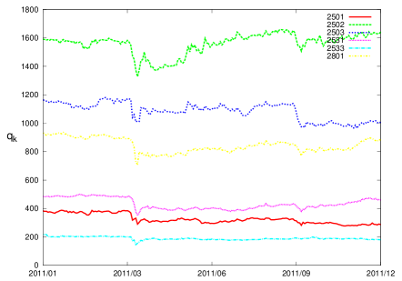
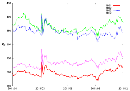
Figure 1: The prices of several major stocks in food industries (left) and construction industries (right) as a function of time (these are daily data sets). Each number shown at each line caption denotes the ID for each company: (i.e. 2501: Sapporo Breweries, 2502: Asahi Breweries, 2503: Kirin Holdings, 2531: Takara Holdings, 2533: Oenon Holdings, 2801: Kikkoman Corporation, 1801: Taisei Corporation, 1802: Obayashi Corporation, 1803: Shimizu Corporation, 1812: Kajima Corporation. These IDs can be checked at the web site [23]) (COLOR ONLINE)

However, it is impossible for us to mention the co-movement of stocks having correlation (with the majority bulk component including themselves) or anti-correlation during the crisis. In Figure 1, we plot the prices of several major stocks in food business (left) and construction business (right) as a function of time (these are daily data sets). From this figure, we find that The price of stocks for the same type of business behaves as correlated time series, whereas for different types of business, say, food industries and construction business, they have apparent any-correlations especially during the crisis.

Hence, it might be quite important for us to make an attempt to bring out more ‘microscopic’ useful information, which is never obtained from the averaged macroscopic quantities such as stock average, about the market. As a candidate of such ‘microscopic information’, we can use the (linear) correlation coefficient based on the two-body interactions between stocks [14, 15, 16, 17, 18, 19, 20, 21]. To make out the mechanism of financial crisis, it might be helpful for us to visualize such correlations in stocks and compare the dynamical behaviour of the correlation before and after crisis.

In this paper, in order to show and explain the hierarchical information cascade, we visualize the correlation of each stock in two-dimension. We specify each location of $K$ stocks from a given set of the $K(K-1)/2$ distances by making use of the so-called multi-dimensional scaling (MDS) [22]. We also propose a theoretical framework to predict several time-series simultaneously by using cross-correlations in financial markets. The justification of this assumption is numerically checked for the empirical Japanese stock data, for instance, those around 11 March 2011, and for foreign currency exchange rates around Greek crisis in spring 2010.

This paper is organized as follows. In section 2, we explain our tools of analysis, namely, the correlation coefficient and multi-dimensional scaling. In section 3, our forecasting model for stock prices is introduced. In section 4, we examine our model for empirical data sets. The last section gives several remarks.

2 Linear correlation coefficient and multi-dimensional scaling

We utilize the linear correlation coefficient to measure the strength of correlation between stocks [15, 16, 17, 18, 19, 20]. The correlation coefficient (Pearson estimator) is calculated as follows.

Let us define $p_{t}^{(i)}(\geq 0)$ as a price of stock $i$ at time $t$. Then, we evaluate the return of the price $p_{t}^{(i)}$ in terms of the logarithmic measurement as

$$\Delta r_{i}(t)\equiv\log p_{t}^{(i)}-\log p_{t-1}^{(i)}.$$ (1)

For the above logarithmically rescaled return, we calculate the moving average over a time window (interval) with width $M$ as

$$\overline{\Delta r_{i}(t)}\equiv\frac{1}{M}\sum_{l=t-M+1}^{t}\Delta r_{i}(l)$$ (2)

for stock $i$, and we also evaluate the two-body correlation between stocks $i,j$ by the following definition

$$\overline{\Delta r_{i}(t)\Delta r_{j}(t)}\equiv\frac{1}{M}\sum_{l=t-M+1}^{t}\Delta r_{i}(l)\Delta r_{j}(l).$$ (3)

Then, the linear correlation coefficient is given by

$$c_{ij}(t) = \frac{\overline{\Delta r_{i}(t)\Delta r_{j}(t)}-(\overline{\Delta r_{i}(t)})(\overline{\Delta r_{j}(t)})}{\sqrt{[\overline{(\Delta r_{i}(t))^{2}}-(\overline{\Delta r_{i}(t)})^{2}][\overline{(\Delta r_{j}(t))^{2}}-(\overline{\Delta r_{j}(t)})^{2}]}}.$$ (4)

2.1 Distribution of linear coefficient

As empirical data set, we pick up 200 stocks including the so-called TOPIX (TOkyo stock Price IndeX) Core30, which consists of typical 30 stock indices being picked up from the view point of ‘current price’ or ‘liquidity’ from the Japanese Nikkei stock market [23]. It should be kept in mind that the data itself is not provided as ‘tick-by-tick’ intra-day data, the minimal time interval of the data is one day (the closing price is given in the data set).

In order to investigate the statistical properties, we evaluate the distribution of the correlation coefficient $P(c)$ and plot the result in Figure 2.

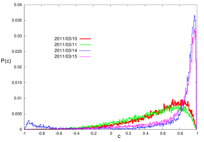
Figure 2: The distribution $P(c)$ of linear correlation coefficients. The result for before crisis (10th, 11th March 2011) and after crisis (14th, 15th March 2011) are shown. It should be noted that 12th and 13th were weekend and the market was closed. We find that a single peak before the crisis splits into the ‘correlated’ (with the majority bulk component including themselves) and ‘anti-correlated’ clusters on 14th. However, the anti-correlated cluster disappears on the next day. (COLOR ONLINE)

From this figure, we clearly find that the distribution is skewed and possesses a single peak at $c>0$ before the crisis. Namely, most of the 200 stocks are mutually correlated. On the other hand, just after the crisis, say, 14th March 2012, the single peak splits into two components and the bulk in which some pairs of two stocks posses the negative correlation appears. Thus, one can grasp the macroscopic aspect of the collective behaviour of the 200 stocks for both before and after the crisis. However, much more microscopic properties of the 200 stocks are unfortunately hided behind the distribution $P(c)$.

To reveal such hidden microscopic aspects of the collective behaviour of the 200 stocks, we shall next attempt to visualize the relationship between these stocks by specifying the location of each stock in two-dimensional space.

2.2 The multi-dimensional scaling: From correlation to distance

To make a plot of the location of each stock, one needs the information about the Euclidean distance between arbitrary two stocks. As we saw in the previous subsection, the correlation coefficient $c_{ij}(t)$ might posses some useful information about the relationship between arbitrary two stocks $i,j$, however, it should be noticed that the correlation coefficient (4) satisfies $-1\leq c_{ij}(t)\leq 1$, and apparently it cannot be treated as a ‘distance’. Hence, here we transform the correlation coefficient $c_{ij}(t)$ into the distance $d_{ij}(t)$ between the stocks $i,j$ as

$$d_{ij}(t)=\sqrt{\frac{1-c_{ij}(t)}{2}}.$$ (5)

We should bear in mind that the above distance satisfies $0\leq d_{ij}(t)\leq 1$ and defines the metric space in multi-dimension [14].

Obviously, once we obtain the location vectors $\bm{X}_{i},\bm{X}_{j}$ for the stocks $i,j$ , one can easily calculate the distance between them as $\|\bm{X}_{i}-\bm{X}_{j}\|$. However, the inverse process, namely, to specify the location vectors $\bm{X}_{i},\bm{X}_{j}$ for a given distance $\|\bm{X}_{i}-\bm{X}_{j}\|$ is not so easy when the number of the stocks $N$ increases. To carry out the inverse process systematically, we can use the well-known method named as multi-dimensional scaling (MDS) (see e.g. [22]). In following, we explain the procedure.

Let us first specify the location of an arbitrary stock $i$ at time $t$ by means of a $P$-dimensional vector $\bm{X}_{i}^{(t)}$ in the following way (Hereafter, we consider the case of $P=2$ especially):

$$\bm{X}_{i}(t)\equiv(x_{i1}(t),x_{i2}(t),\cdots,x_{iP}(t)),\,\,i=1,\cdots,K.$$ (6)

Naturally, the Euclidean distance between arbitrary two stocks $i,j$ is now given by

$$d_{ij}(t)=\sqrt{\sum_{m=1}^{P}(x_{im}(t)-x_{jm}(t))^{2}}.$$ (7)

Hence, the inner product of location vectors of stocks $i$ and $j$ is also calculated as

$$2\{\bm{X}_{i}(t)\cdot\bm{X}_{j}(t)\}=2z_{ij}(t)=\frac{1}{K}\sum_{i=1}^{K}d_{ij}(t)^{2}+\frac{1}{K}\sum_{j=1}^{K}d_{ij}(t)^{2}-\frac{1}{K^{2}}\sum_{i,j=1}^{K}d_{ij}(t)^{2}-d_{ij}(t)^{2}$$ (8)

where we should notice that we chose the origin of axis as the ‘center of mass’ $\bm{X}_{c}(t)$ for $K$ stocks points, that is to say,

$$\bm{X}_{c}(t)\equiv\frac{1}{K}\sum_{i=1}^{K}\bm{X}_{i}(t)=\bm{0}$$ (9)

to specify an arbitrary stock (vector) at each time $t$. This equation (9) implies that the center of mass is a time-independent vector and it is definitely fixed at the origin for all time $t\geq 0$.

Then, in order to look for the locations $\bm{X}_{i}(t),\,i=1\,\cdots,K$ which generates a set of distances $\{d_{ij}(t)\}$ consistently, we should minimize the following energy function (cost):

$$E_{t}=\sum_{i,j=1}^{K}\left(z_{ij}(t)-\sum_{m=1}^{P}x_{im}(t)x_{jm}(t)\right)^{2}$$ (10)

with respect to $\bm{X}_{i}(t),\,i=1,\cdots,K$.

Thus, our problem to find the best possible locations for stocks is now rewritten in terms of an optimization problem to look for the solution $\bm{X}_{i}(t),\,i=1,\cdots,K$ that minimizes the energy function $E_{t}$ at each time step $t$. We plot the result in Figure 3 for the same data set used in the plot of Figure 2.

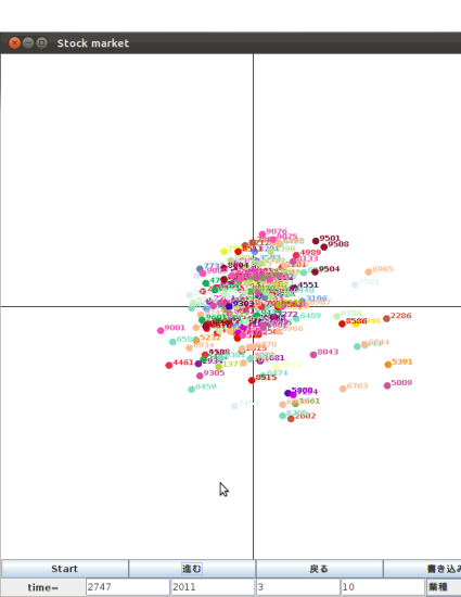
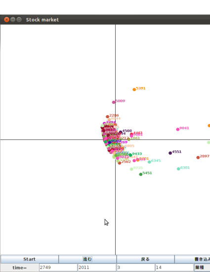
Figure 3: The result of the MDS. We pick up 200 stocks including the so-called TOPIX Core30 and the Nikkei stock average as empirical data set. The results on 10th (left) and 14th (right) March 2011 are shown. Different colors indicate different types of business. The numbers accompanying the dots show company IDs. The isolated points anti-correlated with the bulk are construction business, such as 1934: Yurtec Corporation, which is a construction industry in Tohoku area, 1826: Sata Construction Co. Ltd. We set the width of time window to evaluate the correlation coefficient as $M=7$ (days). (COLOR ONLINE)

From these panels, we clearly find that after the crisis, the scattered plots actually shrink into a small limited region centered at the origin (the center of mass) as we expected before. Isolated several dots separating from main clusters denote the price of ‘building industry’. These isolated points anti-correlated with the bulk are construction business, such as ID 1934: Yurtec corporation, which is a construction industry in Tohoku area, ID 1826: Sata construction Co. Ltd. Apparently we recognize that the large amount of demand is expected in such industries even after the crisis (mega earthquakes).

3 Prediction by using cross-correlation

It is necessary for us to investigate the human collective behaviour of the social agents such as traders in order to construct persistent systems in earthquake disasters. In financial systems, the price of each commodity as a macroscopic quantity is determined by huge number of trader’s making decisions. To predict the price efficiently, a lot of mathematical tools such as AR model and its extensions called as ARCH model or GARCH model [6], or Kalman filter and its various variants have been proposed. Recently, besides these rather traditional models, several physics inspired models have been also introduced by several authors [24, 25, 26]. However, these models apparently lack the microscopic view point. Namely, in these models, the predicted price is not constructed by the result from microscopic trader’s decision making.

Among these studies of prediction of stock prices, Kaizoji [27] attempted to represent ‘buying’ and ‘selling’ signals posted by traders by ‘Ising spin’. He proposed a model in which the return of the price is determined by the ‘magnetization’ of the Ising system. He carried out computer simulations and concluded that there are interesting relationship between financial phenomena such as ‘bubble’ or ‘crush’ and physically collective phenomena which are referred to as ‘phase transition’ in the Ising magnetic system.

However, those studies seem to be not yet extensive and there exist several open questions to be clarified. For instance, dynamics of macroscopic quantities which might specify the collective behaviour of traders should be revealed more extensively. And as we saw in the previous sections, just after crisis, several stocks are strongly correlated. Hence, we might use the cross-correlation to predict several prices simultaneously by modifying the Kaizoji’s model [27] by means of the cross-correlations. Therefore, from this section, we are focusing on the prediction of prices of several stocks simultaneously by using the cross-correlation in stock markets.

3.1 A link from microscopic making decisions to macroscopic prices

In order to investigate the effect of the cross-correlation on the prediction of several stock-prices, we first explain the model proposed by Kaizoji [27] as a basic model.

Let us define $p_{t}^{(k)}$ as the price of commodity $k$ at time $t$. Then, the return, which is defined as the difference between prices at successive two time steps $t$ and $t+1$ is given by

$$\Delta p_{t}^{(k)}\equiv p_{t+1}^{(k)}-p_{t}^{(k)}=m^{(k)}_{t},\,\,\,k=1,\cdots,K.$$ (11)

In order to construct the return $m_{t}^{(k)}$ from the microscopic view point, we assume that each trader ($i=1,\cdots,N_{k}$) possessing the stock $k$ buys or sells $v_{it}^{(k)}$-volumes at each time step $t$. Then, let us call the group of buyers as $\mathcal{A}_{+}(k,t)$, whereas the group of sellers is referred to as $\mathcal{A}_{-}(k,t)$. Hence, the total volumes of buying and selling are explicitly given by

$$\psi_{+}(k,t)\equiv\sum_{i\in\mathcal{A}_{+}(k,t)}v_{it}^{(k)},\,\,\psi_{-}(k,t)\equiv\sum_{i\in\mathcal{A}_{-}(k,t)}v_{it}^{(k)},$$ (12)

respectively. We should keep in mind that the total number of traders dealing with the stock $k$ is conserved, namely, the condition:

$$\mathcal{A}_{+}(k,t)+\mathcal{A}_{-}(k,t)=N_{k}$$ (13)

should be satisfied.

Then, the return $m_{t}^{(k)}$ is naturally defined by means of (12)

$$m_{t}=\lambda(\psi_{+}(k,t)-\psi_{-}(k,t))$$ (14)

where $\lambda$ is a positive constant. Namely, when the volume of buyers is greater than that of sellers, $\psi_{+}(k,t)>\psi_{-}(k,t)$, the return becomes positive $m_{t}^{(k)}>0$. As the result, the price of the commodity $k$ should be increased at the next time step as $\Delta p_{t}^{(k)}=m_{t}^{(k)}$.

3.1.1 Ising spin representation

The above microscopic observation and the set-up might be naturally accepted, however, here we shall make the situation much more simpler. Namely, we omit the information about the volume by setting $v_{it}^{(k)}=1\,(\forall_{i,t,k})$. The making decision of each trader ($i=1,\cdots,N_{k}$) is now obtained simply by an Ising spin:

$$S_{i}^{(k)}(t)=\left\{\begin{array}[]{cc}+1&\mbox{(the trader $i$ buys the stock $k$ at time $t$)}\\ -1&\mbox{(the trader $i$ sells the stock $k$ at time $t$)}\end{array}\right.$$ (15)

The return is also simplified as

$$m_{t}^{(k)}=\lambda(\psi_{+}(k,t)-\psi_{-}(k,t))=\lambda\sum_{i=1}^{N_{k}}v_{it}^{(k)}S_{i}^{(k)}(t)$$ (16)

where we set $\lambda=N_{k}^{-1}$ to make the return:

$$m_{t}^{(k)}=\frac{1}{N_{k}}\sum_{i=1}^{N}S_{i}^{(k)}(t)$$ (17)

satisfying $|m_{t}^{(t)}|\leq 1$. Thus, $m_{t}^{k}$ corresponds to the ‘magnetization’ in statistical physics, and the update rule of the price for the stock $k$ is governed in terms of the magnetization $m_{t}^{(k)}$ as

$$\Delta p_{t}^{(k)}=m_{t}^{(k)},\,k=1,\cdots,K.$$ (18)

3.2 The energy function

We next introduce the energy function of the system.

$$E_{t}(\bm{S}^{(k)})=-\frac{J_{t}^{(k)}}{N_{k}}\sum_{ij}S_{i}^{(k)}S_{j}^{(k)}-h_{t}^{(k)}\sum_{i}\sigma_{\tau}^{(k)}(t)S_{i}^{(k)}-\gamma_{t}^{(k)}\sum_{i}\left(\frac{1}{K}\sum_{\mu\neq k}^{K}c_{k\mu}(t)m_{t}^{(\mu)}\right)S_{i}^{(k)}$$ (19)

where we omitted the time dependence in $S_{i}^{(k)}$ for simplicity. The first term in the right hand side of (19) induces human collective behaviour, namely, each agent inclines to take the same decision as the others to decrease the total energy. The effect of this first term on the minimization of total energy might be recognized as the so-called Keynes’s beauty contest. It means that traders tend to make the same decision as the others, in particular, during a crisis. Namely, when a big negative news (mood) such as earthquake in Japan is broadcasted, almost all of the traders might sell their own stocks as the others also sell without any rationality. In other words, the first term causes the human collective behaviour of the traders, which is sometimes refereed to as information cascade in the literature of behavioral economics, for $J_{t}^{(k)}\geq h_{t}^{(k)},\gamma_{t}$. Actually, we find that the lower bound of the first term in the right hand side of (19) is evaluated as

$$-\frac{J_{t}^{(k)}}{N_{k}}\sum_{ij}S_{i}^{(k)}S_{j}^{(k)}\geq-N_{k}J_{t}^{(k)}$$ (20)

where the equal sign is satisfied if and only if $S_{i}^{(k)}=1\,\,(\forall_{i})$ or $S_{i}^{(k)}=-1\,\,(\forall_{i})$ holds.

The second term in (19) represents the cross-correlation between the decisions of traders and market (historical) information. In this paper, we choose the ‘trends’ :

$$\sigma_{\tau}^{(k)}(t)\equiv\frac{p_{t}-p_{t-\tau}}{\tau}$$ (21)

for such information. This means that the total energy should decrease when each trader posts the sign $S_{i}^{(k)}=\pm 1$ to the market so as to make the product $\sigma_{\tau}^{(k)}(t)S_{i}^{(k)}$ definitely positive. In other words, each trader buys the commodity $k$ if the price tends to increase over the past $\tau$-time steps, whereas the trader sells the stock vice versa. Actually, the second term is definitely minimized as

$$-h_{t}^{(k)}\sum_{i}\sigma_{\tau}^{(k)}(t)S_{i}^{(k)}\geq-N_{k}h_{t}^{(k)}|\sigma_{\tau}^{(k)}(t)|$$ (22)

where the equality should be satisfied when ${\rm sgn}[S_{i}^{(k)}]={\rm sgn}[\sigma_{\tau}^{(k)}(t)]$ holds.

The third term, which does not appear in the references [27], comes from correlation between the trader $i$ possessing the commodity $k$ and a ‘typical trader’ (a mean-field) $m_{t}^{(\mu)}$ possessing stocks $\mu\,(\neq k)$. A factor $c_{k\mu}(t)$ appearing in the third term stands for the correlation coefficient and we should remember that it is given by (4) explicitly. Hence, when the stocks $k$ and $\mu$ are correlated in terms of the positive coefficient, namely, $c_{k\mu}(t)>0$ from time $t-M+1$ to time $t$, the trader possessing the stock $k$ inclines to take the same decision as the typical trader dealing with the stock $\mu$, that is, $m_{t}^{(\mu)}$.

From the above argument, it might be useful for us to investigate to what extent those traders behave collectively through the values of macroscopic hyper-parameters $J_{t}^{(k)},h_{t}^{(k)}$ and $\gamma_{t}^{(k)}$. Namely, in the realistic stock market, there might exist a possibility that human behaviour turns out to be collective and ‘irrational’ in some sense when these parameters change the values as $h_{t}^{(k)}/J_{t}^{(k)}\to 0,\gamma_{t}^{(k)}/J_{t}^{(k)}\to 0$ and $J_{t}^{(k)}\to 1$ (a critical point of infinite range ferromagnetic Ising model).

3.3 The Boltzmann-Gibbs distribution

It should be noticed that the state vectors of the agents: $\bm{S}^{(k)}=(S_{1},\cdots,S_{N_{k}}),\,\,k=1,\cdots,K$ are determined so as to minimize the energy function (19) from the argument in the previous subsection. For most of the cases, the solution should be unique. However, in realistic financial markets, the decisions by agents should be much more ‘diverse’. Thus, here we consider statistical ensemble of traders for each commodity $\bm{S}^{(k)}$ and define the distribution of the ensemble by $P(\bm{S}^{(k)})$. Then, we shall look for the suitable distribution which maximizes the so-called Shannon’s entropy

$$H=-\sum_{\bm{S}^{(k)}}P(\bm{S}^{(k)})\log P(\bm{S}^{(k)})$$ (23)

under two distinct constraints:

$$\sum_{\bm{S}^{(k)}}P(\bm{S}^{(k)})=1,\,\,\sum_{\bm{S}^{(k)}}P(\bm{S}^{(k)})E(\bm{S}^{(k)})=E_{k}.$$ (24)

Namely, according to Jaynes [28], we choose the distribution which minimizes the following functional $f_{k}\{P(\bm{S}^{(k)})\}$:

$$f_{k}\{P(\bm{S}^{(k)})\} = -\sum_{\bm{S}^{(k)}}P(\bm{S}^{(k)})\log P(\bm{S}^{(k)})-\lambda_{1}^{(k)}\left(\sum_{\bm{S}^{(k)}}P(\bm{S}^{(k)})-1\right)$$ (25)

$$- \lambda_{2}^{(k)}\left(\sum_{\bm{S}^{(k)}}P(\bm{S}^{(k)})E_{k}(\bm{S}^{(k)})-E_{k}\right)$$

where $\lambda_{1}^{(k)},\lambda_{2}^{(k)}$ are Lagrange’s multipliers. After some easy algebra, we immediately notice that $\lambda_{1}^{(k)}$ gives a normalization constant of $P(\bm{S}^{(k)})$ and $\lambda_{2}^{(k)}\equiv\beta$ is a control parameter for ‘thermal fluctuation’ in the system. Thus, we have the solution as

$$P(\bm{S}^{(k)})=\frac{{\exp}[-\beta E(\bm{S}^{(k)})]}{\sum_{\bm{S}^{(k)}}{\exp}[-\beta E(\bm{S}^{(k)})]}$$ (26)

where $\beta$ stands for the inverse-temperature, and hereafter we set $\beta=1$. We also defined the sum with respect to $\bm{S}^{(k)}$ by

$$\sum_{\bm{S}^{(k)}}(\cdots)\equiv\sum_{S_{1}^{(k)}=\pm 1}\cdots\sum_{S_{N}^{(k)}=\pm 1}(\cdots).$$ (27)

3.4 A Bayesian interpretation

It might be helpful for us to interpret the above probability distribution (26) from the view point of Bayesian inference. Actually, one can derive the above Boltzmann-Gibbs form $P(\bm{S}^{(k)})$ by means of a posterior distribution in Bayesian statistics. Let us assume that the price change of stock might be caused by $\sigma_{\tau}^{(k)}(t)$ due to the microscopic decision making $S_{i}^{(k)}=\pm 1$ for trader $i$. Then, the following conditional probability

$$P(\sigma_{\tau}^{(k)}(t)|\bm{S}^{(k)})\propto{\exp}\left(h_{t}^{(k)}\sum_{i=1}^{N}\sigma_{\tau}^{(k)}(t)S_{i}^{(k)}\right)$$ (28)

denotes a likelihood of the result $\sigma_{\tau}^{(k)}(t)$ caused by the decision making of traders $\bm{S}^{(k)}$. Therefore, in order to forecast the decision of traders $\bm{S}^{(k)}$ for a given market data $\sigma_{\tau}^{(k)}(t)$, we construct the posterior $P(\bm{S}^{(k)}|\sigma_{\tau}^{(k)}(t))$ by means of the Bayesian formula

$$P(\bm{S}^{(k)}|\sigma_{\tau}^{(k)}(t))\propto P(\sigma_{\tau}^{(k)}(t)|\bm{S}^{(k)})Q(\bm{S}^{(k)}|\{m_{t}^{(\mu\neq k)}\})$$ (29)

where $Q(\bm{S}^{(k)}|\{m_{t}^{(\mu\neq k)}\})$ stands for the prior distribution. For a given set of mean-fields from the other Ising layers $\{m_{t}^{(\mu\neq k)}\}$, it is naturally accepted to choose the prior as

$$Q(\bm{S}^{(k)}|\{m_{t}^{(\mu\neq k)}\})\propto{\exp}\left[\frac{J_{t}^{(k)}}{N_{k}}\sum_{ij}S_{i}^{(k)}S_{j}^{(k)}+\gamma_{t}^{(k)}\sum_{i}\left(\frac{1}{K}\sum_{\mu\neq k}^{K}c_{k\mu}(t)m_{t}^{(\mu)}\right)S_{i}^{(k)}\right]$$ (30)

Then, we have the posterior

$$\fl P(\bm{S}^{(k)}|\sigma_{\tau}^{(k)}(t))$$

$$= \frac{{\exp}[\frac{J_{t}^{(k)}}{N_{k}}\sum_{ij}S_{i}^{(k)}S_{j}^{(k)}+h_{t}^{(k)}\sum_{i}\sigma_{\tau}^{(k)}(t)S_{i}^{(k)}+\gamma_{t}^{(k)}\sum_{i}(\frac{1}{K}\sum_{\mu\neq k}^{K}c_{k\mu}(t)m_{t}^{(\mu)})S_{i}^{(k)}]}{\sum_{\bm{S}^{(k)}}{\exp}[\frac{J_{t}^{(k)}}{N_{k}}\sum_{ij}S_{i}^{(k)}S_{j}^{(k)}+h_{t}^{(k)}\sum_{i}\sigma_{\tau}^{(k)}(t)S_{i}^{(k)}+\gamma_{t}^{(k)}\sum_{i}(\frac{1}{K}\sum_{\mu\neq k}^{K}c_{k\mu}(t)m_{t}^{(\mu)})S_{i}^{(k)}]}.$$

Thus, our model system is described by multi-layered Ising model in which arbitrary two layers (stocks) are coupled through the mean-fields.

3.5 The mean-field equation for instantaneous return

As it is well-known, when ingredients of the system are ‘fully-connected’, the partition function $Z$ (the numerator of (LABEL:eq:posterior)) is evaluated at the saddle point as

$$Z\simeq{\exp}\left[N_{k}\Phi(m^{(k)}:J_{t}^{(k)},h_{t}^{(k)},\gamma_{t}^{(k)},\{m_{t}^{(\mu)}\})\right]$$ (32)

in the limit of $N_{k}\to\infty$ with ‘free energy density’

$$\Phi=-\frac{J_{t}^{(k)}}{2}(m^{(k)})^{2}+\log\cosh\left(J_{t}^{(k)}m^{(k)}+h_{t}^{(k)}\sigma_{\tau}^{(k)}(t)+\frac{\gamma_{t}^{(k)}}{K}\sum_{\mu\neq k}^{K}c_{k\mu}(t)m_{t}^{(\mu)}\right).$$ (33)

Thus, the saddle point equation $\partial\Phi/\partial m^{(k)}=0$ yields

$$m^{(k)}=\tanh\left(J_{t}^{(k)}m^{(k)}+h_{t}^{(k)}\sigma_{\tau}^{(k)}(t)+\frac{\gamma_{t}^{(k)}}{K}\sum_{\mu\neq k}^{K}c_{k\mu}(t)m_{t}^{(\mu)}\right).$$ (34)

The second and third terms appearing in $\tanh(\cdots)$ are an external field from the market history and mean-fields from the other Ising layers, respectively. For a given non-stationary field $\sigma_{t}^{(k)}(t)$ and mean-field $\{m_{t}^{(\mu)}\}$, it could not be expected that the equilibrium solution for each layer $m^{(k)}$ exists. Hence, here we assume that such non-equilibrium effects could be built-in by dealing with the following time-dependent (naive) mean-field equation for the ‘instantaneous’ returns.

$$m_{t}^{(k)}=\tanh\left(J_{t-1}^{(k)}m_{t-1}^{(k)}+h_{t-1}^{(k)}\sigma_{\tau}^{(k)}(t-1)+\frac{\gamma_{t-1}^{(k)}}{K}\sum_{\mu\neq k}^{K}c_{k\mu}(t-1)m_{t-1}^{(\mu)}\right),\,\,k=1,\cdots,K$$ (35)

By solving the above non-linear maps numerically for a given set of past real market history $\{\sigma_{\tau}^{(k)}(t-1)\}$, one can forecast the price of each stock by means of $\Delta p_{t}=m_{t}^{(k)},\,\,k=1,\cdots,K$ simultaneously.

3.6 Hyper-parameter estimation from non-stationary time-series

In order to use the mean-field equation (35) for forecasting the stock prices, systematic estimation for the so-called hyper-parameters $(J_{t}^{(k)},h_{t}^{(k)},\gamma_{t}^{(k)})$ appearing in the right hand side of (35) is needed. In the literature of probabilistic information processing, say, in Bayesian image restoration [29], one cannot use the mean-square error as a cost function because it needs the ‘true (original) image’ to be constructed. Therefore, we usually use the marginal likelihood as the cost function to estimate the hyper-parameters. However, fortunately in our present model system, one can utilize the past market history, let us to say, the ‘true returns’ in the past $\Delta q_{l}^{(k)}\equiv q_{l}^{(k)}-q_{l-1}^{(k)},\,\,l=1,\cdots,t-1$, and it means that the ‘cumulative error’ could be defined as a cumulative mean-square error between the true observable and the estimate by

$$\mathcal{E}_{k} \equiv \frac{1}{2}\sum_{l=1}^{t-1}\left(\overline{\Delta q_{l}^{(k)}}-\overline{\Delta p_{l}^{(k)}}\right)^{2}$$ (36)

$$= \frac{1}{2}\sum_{l=1}^{t-1}{\Biggr{[}}\overline{\Delta q_{l}^{(k)}}-\tanh{\Biggr{(}}J_{t-1}^{(k)}\overline{\Delta q_{l-1}^{(k)}}+h_{t-1}^{(k)}\sigma_{\tau}^{(k)}(t-1)+\frac{\gamma_{t-1}^{(k)}}{K}\sum_{\mu=1}^{K}c_{k\mu}(t-1)\overline{\Delta q_{l-1}^{(\mu)}}{\Biggr{)}}{\Biggr{]}}^{2}$$

where we defined the ‘forecasted return’ $\Delta p_{l}^{(k)}\equiv p_{l}^{(k)}-p_{l-1}^{(k)},\,\,l=1,\cdots,t-1$ and the time-averages

$$\overline{\Delta q_{l}^{(k)}}\equiv\frac{1}{M}\sum_{i=l-M+1}^{l}(q_{i+1}^{(k)}-q_{i}^{(k)}),\,\,\overline{\Delta p_{l}^{(k)}}\equiv\frac{1}{M}\sum_{i=l-M+1}^{l}(p_{i+1}^{(k)}-p_{i}^{(k)})$$ (37)

for the time window with width $M$. To obtain the last line in the above equation (36), we used

$$\overline{\Delta p_{l}^{(k)}}\simeq m_{l}^{(k)}=\tanh\left(J_{t-1}^{(k)}m_{l-1}^{(k)}+h_{t-1}^{(k)}\sigma_{\tau}^{(k)}(t-1)+\frac{\gamma_{t-1}^{(k)}}{K}\sum_{\mu\neq k}^{K}c_{k\mu}(t-1)m_{l-1}^{(\mu)}\right)$$ (38)

and replaced the $m_{l-1}^{(k)},\,k=1,\cdots,K$ appearing in $\tanh(\cdots)$ by the corresponding observables $\overline{\Delta q_{l-1}^{(k)}},\,k=1,\cdots,K$ because one can actually use these values before forecasting.

Hence, we should infer these hyper-parameters $(J_{t}^{(k)},h_{t}^{(k)},\gamma_{t}^{(k)})$ from the past data set in the financial market by the gradient descent learning

$$J_{t}^{(k)}=J_{t-1}^{(k)}-\eta\,\frac{\partial\mathcal{E}_{k}}{\partial J_{t-1}^{(k)}},\,\,h_{t}^{(k)}=h_{t-1}^{(k)}-\eta\,\frac{\partial\mathcal{E}_{k}}{\partial h_{t-1}^{(k)}},\,\,\gamma_{t}^{(k)}=\gamma_{t-1}^{(k)}-\eta\,\frac{\partial\mathcal{E}_{k}}{\partial\gamma_{t-1}^{(k)}},$$ (39)

where $\eta$ is a learning rate. In the next section, we examine the above forecasting framework for empirical (intra-day) data sets in which a crisis appears.

4 Performance evaluation of forecasting for empirical high-frequency data sets

In this section, we check the usefulness of our prediction model with cross-correlation in stocks. As a simple examination, for the case of three different time-series $K=3$, we check the accuracy of our prediction procedure. In section 2, we visualized 200 stocks which are given as daily data during a crisis. However, the number of data points is not enough for our forecasting procedure. Hence, here we pick up EUR/AUD ($k=1$), EUR/CAD ($k=2$), EUR/JPY ($k=3$) exchange rates (EUR: Euro, CAD: Canadian dollar, AUD: Australian dollar, JPY: Japanese yen), which are given as high-frequency tick-by-tick data, from 27th April 2010 to 13th May 2010 as real values $q_{t}^{(k)}$. We plot those three true time series in Figure 4 as solid lines. We observe that these time series posses a crisis which corresponds to Greek crisis in spring 2010. In the left panels of Figure 4, the resulting prices $p_{t}^{(k)}$ predicted by our model are shown. We set the time window size as $M=\tau=100$ and the learning rate as $\eta=0.01$. Of course, we can choose the leaning rate as ‘adaptive one’ like $\eta=\eta(t)$, however, in this paper we set the value to a positive constant. From these panels, we find that our prediction procedure works well and the error is only a few percent of the average value of the rate.

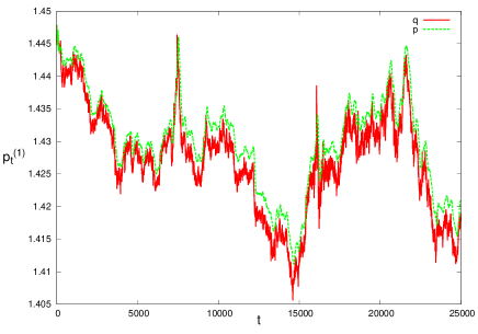
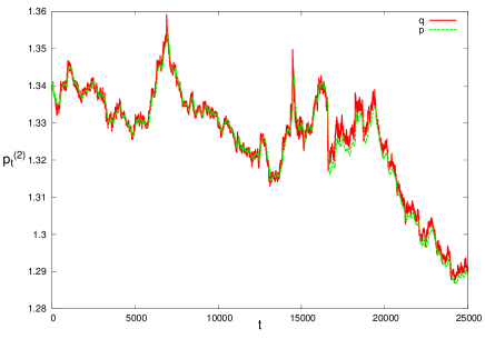
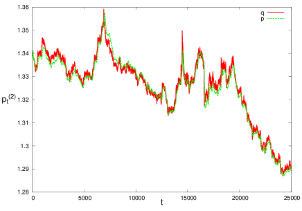
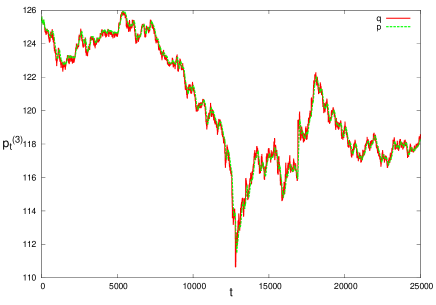
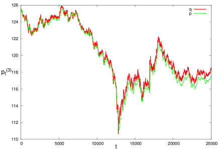
Figure 4: From the top to the bottom, EUR/AUD ($k=1$), real value $q_{t}^{(k)}$ and its prediction $p_{t}^{(k)}$ are plotted for EUR/CAD ($k=2$), EUR/JPY ($k=3$) exchange rates from 27th April 2010 to 13th May 2010. The panels in the left column are obtained by ‘stock-wise optimization’, whereas the panels in the right are calculated by ‘pair-wise optimization’ for the correlation strengths. We set the width of time window and the learning rate as $M=\tau=100,\eta=0.01$. (COLOR ONLINE)

4.1 Pair-wise optimization for hyper-parameters of correlation strengths

We next examine the following slight modification

$$\frac{\gamma_{t}^{(k)}}{K}\sum_{\mu\neq k}^{K}c_{k\mu}(t-1)\overline{\Delta q_{l-1}^{(\mu)}}\to\frac{1}{K}\sum_{\mu\neq k}^{K}\gamma_{t}^{(k\mu)}c_{k\mu}(t-1)\overline{\Delta q_{l-1}^{(\mu)}}$$ (40)

in (35)-(36). Namely, the strength of correlation between Ising layers is evaluated independently for each pair of layers. Due to this modification, the learning equation for $\gamma_{t}^{(k)}$ in (39) should be corrected as

$$\gamma_{t}^{(k\mu)}=\gamma_{t-1}^{(k\mu)}-\eta\,\frac{\partial\mathcal{E}_{k}}{\partial\gamma_{t-1}^{(k\mu)}},\,\mu\neq k.$$ (41)

From now on, the forecasting model with the above modification (40)(41) is referred to as ‘pair-wise optimization’, whereas the original version (35)(36) is called as ‘stock-wise optimization’ for hyper-parameters for the correlation strengths.

We plot the result in the right panels in Figure 4. From these panels, we are confirmed that the pair-wise optimization makes the result worse against our expectation. Especially, for large $t$ regime, the gap between the stock-wise optimization and the pair-wise optimization becomes large. From the result, we should consider the optimal number of hyper-parameters to fit the model to the time-series without over-fitting.

4.2 Flows of hyper-parameters during a crisis

Finally, we consider the dynamical behaviour of hyper-parameters during the crisis. We show the results in Figure 5.

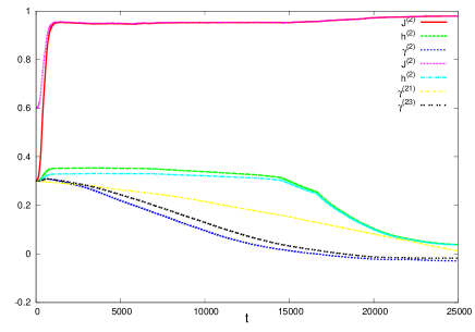
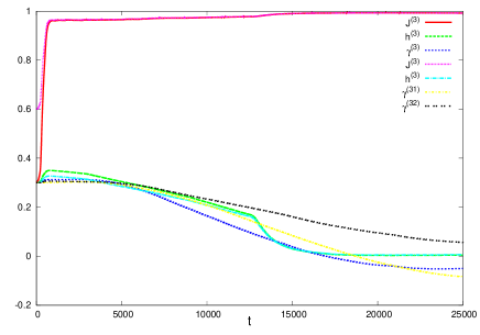
Figure 5: Dynamics of macroscopic parameters $(J_{t}^{(k)},h_{t}^{(k)},\gamma_{t}^{(k)})$ for ‘stock-wise optimization’ (The top three line captions) and $(J_{t}^{(k)},h_{t}^{(k)},\gamma_{t}^{(k\mu)})$ for ‘pair-wise optimization’ (The bottom four line captions). We show the result for $k=2$ (left panel) and $k=3$ (right). (COLOR ONLINE)

These panel show the dynamics of hyper-parameters $(J_{t}^{(k)},h_{t}^{(k)},\gamma_{t}^{(k)})$ for the stock-wise optimization and and $(J_{t}^{(k)},h_{t}^{(k)},\gamma_{t}^{(k\mu)})$ for the pair-wise optimization.

From this panel, we clearly find that for both cases $(k=2,3)$ of exchange rates in our forecasting model described by stock-wise optimization, the hyper-parameters $J^{(k)},h^{(k)}$ converge to $h^{(k)}=0$ and $J^{(k)}=1$, respectively. Then, the $\gamma_{t}^{(k)}$ converges to zero for $k=2$, which corresponds to the critical point of order-disorder phase transition in the infinite-range ferromagnetic Ising model. However, for $k=3$ it converges to slightly negative value across the zero. Hence for $k=3$ the stock-wise optimization does not detect the critical behaviour, and the deviation from the critical point becomes large as $t$ goes on. On the other hand, the model with the pair-wise optimization also detects the critical behaviour for $k=2$, however, the behavior of the hyper-parameters does not reflect the critical point (crisis) for $k=3$.

We can partially figure out these results in the original time series shown in Figure 4. From this figure, we can observe that the exchange rate $k=3$ was recovered from the crisis relatively faster than $k=2$, whereas it was still in a crisis for the exchange rate $k=2$ even in large $t$ regime. Actually, in this period, Japanese yen was strong, and at the crisis, this tendency of strong yen was enhanced. However, the term of extreme strong yen is not so long and the value of Euro against yen was recovered quickly. On the other hand, continuous drops of Euro against Canadian dollar was serious after the crisis and it could not escape from a ‘crush domain’ even at $t=250000$ (ticks). In this sense, the deviation from the critical point should be also observed through our model and actually it was confirmed in Figure 5.

5 Discussions and concluding remarks

There are many ways to visualize the co-movements of stocks, and using MDS is one of them. When the MDS studies were performed with daily data [35], we found that it was easier to visualize or detect specific sectors, strongly correlated pairs and market events. It was suggested that this type of plots using daily data may be used in designing strategies of “pairs trade” or identifying clusters or detecting market trends. It was also shown in Ref. [35], that we could follow the evolution of the market and/or trace the movements of particular companies (e.g., Lehmann Brothers) with respect to the rest of the market, before or after a market crisis.

In this paper, in order to show and forecast some cascade in financial systems, we visualized the correlation of each pair of stocks in two-dimension using MDS. We also proposed a theoretical framework based on the multi-layered Ising model to predict several time-series simultaneously by using cross-correlations in financial markets. Actually, in this paper, we showed that the knowledge of statistical mechanics of information (see e.g. [30]) could be applicable to the research topics outside of information processing, namely, quantitative finance or economics.

Finally, we would like to mention several remarks concerning our future direction.

5.1 On the time window size

In our model system, we set $M=\tau=100$ for the width of time window to evaluate several statistics in our forecasting model (see (21) and (37)). However, we should chose these lengths more carefully. Recently, Livan, Inoue and Scalas [31] examined the effect of non-stationarity of time series on the portfolio optimization by using several statistical test including some knowledge of the random matrix theory [32], and they found that the longer time window does not always give the better estimate of the true value of the portfolio. This implies that there might exist some optimal size of window to construct the forecasting model.

5.2 The turnover

The turnover, namely, the total number of volume being dealt with for a stock at time $t$:

$$a_{k}(t)\equiv\psi_{+}(k,t)+\psi_{-}(k,t)=\sum_{i=1}^{N_{k}}v_{it}^{(k)}$$ (42)

might be a good indicator for the financial crisis (see also (12)). Actually, in Figure 6, we show the empirical plot of the turnover for several stocks during the crisis in Japan 2011. From this figure, we find that the turnover takes a sharp peak around the shock (11th March 2011), which was remarkably observed in stocks of construction industries (see the right panel of Figure 6). In our preliminary study [33], we made a model to estimate the turnover by means of three state Ising model in which each spin can take zero (‘staying’) besides $\pm 1$ for ‘selling’ or ‘buying’.

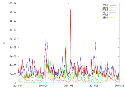
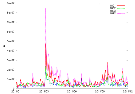
Figure 6: The turnover as a function of time (day). The number of caption denotes the ID for each company: (i.e. 2501: Sapporo Breweries, 2502: Asahi Breweries, 2503: Kirin Holdings, 2531: Takara Holdings, 2533: Oenon Holdings, 2801: Kikkoman Corporation, 1801: Taisei Corporation, 1802: Obayashi Corporation, 1803: Shimizu Corporation, 1812: Kajima Corporation. These IDs can be checked at the web site [23]) (COLOR ONLINE)

5.3 Suitable estimator for non-synchronous time series

The data sets used in the forecasting examination are not daily data but high-frequency data. Those are ‘non-synchronous’ time series, namely, there is no one-to-one correspondence in time axis in arbitrary two stocks. In this paper, for evaluating, say, $\Delta r_{i}(t)\Delta r_{j}(t^{{}^{\prime}})$ where $t\neq t^{{}^{\prime}}$, we chose the $t^{{}^{\prime}}$ simply by

$$t^{{}^{\prime}}={\rm argmin}_{t}\|t-t^{{}^{\prime}}\|$$ (43)

and of course, it might posses some evaluation error. In this sense (namely, ‘strict sense’), the Pearson estimator is not suitable to evaluate the cross-correlation, and we should use another way, say, the so-called Hayashi-Yoshida estimator [34, 35].

5.4 The inverse-Ising problem

In our forecasting model, we assumed that the traders are fully-connected. However, the graph topology is important for us to consider the communities in the markets. Hence, the procedure to estimate the adjacency matrix from the empirical data (behavior of traders) should be done. Definitely, it is formulated as an ‘inverse Ising problem’.

The studies related to the above four issues are now on-going and we will report the results at the meeting if we obtain the preliminary.

References

References

- [1] Cont R 2001 Quantitative Finance 1 223
- [2] Chakraborti A, Muni Toke I, Patriarca M and Abergel F 2011 Quantitative Finance 11 991
- [3] Chakraborti A, Muni Toke I, Patriarca M and Abergel F 2011 Quantitative Finance 11 1013
- [4] Chakraborti A, Patriarca M and Santhanam M S 2007 Econophysics of Markets and Business Networks (Milan: Springer) p 51
- [5] Bouchaud J P and Potters M 2000 Theory of Financial Risk and Derivative Pricing (Cambridge: Cambridge University Press)
- [6] Mantegna R N and Stanley H E 2000 An Introduction to Econophysics (Cambridge: Cambridge University Press)
- [7] Garibaldi U and Scalas E 2010 Finitary Probabilistic Methods in Econophysics (Cambridge: Cambridge University Press)
- [8] Aoyama H, Fujiwara Y, Ikeda Y, Iyetomi H, Souma W and Yoshikawa H 2011 Econophysics and Companies: Statistical Life and Death in Complex Business Networks (Cambridge: Cambridge University Press)
- [9] Sinha S, Chatterjee A, Chakraborti A and Chakrabarti B K 2011 Econophysics: An Introduction (Berlin: Wiley-VCH)
- [10] Chakrabarti B K, Chakraborti A, Chakravarty S R and Chatterjee A 2013 Econophysics of Income and Wealth Distributions (Cambridge: Cambridge University Press)
- [11] Eds. Chakrabarti B K, Chakraborti A and Chatterjee A 2006 Econophysics and Sociophysics: Trends and Perspectives (Weinheim: Wiley-VCH)
- [12] Keim D B 1983 J. Financial Economics 12 13
- [13] Kahneman D and Tversky A 1979 Econometrica 47 263
- [14] Ibuki T, Suzuki S and Inoue J 2012 Econophysics of Systemic Risk and Network Dynamics (Milan: Springer) p 239
- [15] Mantegna R N 1999 Eur. Phys. J. B 11 193
- [16] Onnela J-P, Chakraborti A, Kaski K, Kertesz J and Kanto A 2003 Phys. Rev. E 68 056110
- [17] Chakraborti A 2006 Econophysics of Stock and other Markets (Milan: Springer) p 13
- [18] Onnela J-P, Chakraborti A, Kaski K, Kertesz J and Kanto A 2003 Physica Scripta T 106 48
- [19] Onnela J-P, Chakraborti A, Kaski K and Kertesz J 2003 Physica A 324 247
- [20] Onnela J-P, Chakraborti A, Kaski K and Kertesz J 2002 Eur. Phys. J. B 30 285
- [21] Ibuki T, Higano S, Suzuki S and Inoue J 2012 ASE Human Journal 1 74
- [22] Borg I and Groenen P 2005 Modern Multidimensional Scaling: theory and applications (New York: Springer)
- [23] http://finance.yahoo.co.jp/
- [24] Bouchaud J P and Cont R 1998 Eur. Phys. J. B 6 543
- [25] Masukawa J 2002 Journal of the Japan Society for Simulation Technology 21 92
- [26] Watanabe K, Takayasu H and Takayasu M 2009 Physical Review E 80 056110
- [27] Kaizoji T 2000 Physica A 287 493
- [28] Jaynes T E 1957 Physical Review 106 620
- [29] Inoue J and Tanaka K 2002 Phys. Rev. E 65 016125
- [30] Nishimori H 2001 Statistical Physics of Spin Glasses and Information Processing: An Introduction (Oxford: Oxford University Press)
- [31] Livan G, Inoue J and Scalas E 2012 J. Stat. Mech.: Theory and Experiment P07025
- [32] Livan G, Alfarano S and Scalas E 2011 Phys. Rev. E 84 016113
- [33] Murota M and Inoue J 2013 Econophysics of Agent-based Models (Milan: Springer) in press
- [34] Hayashi T and Yoshida N 2005 Bernoulli 11 359
- [35] Tilak G, Szll T, Chicheportiche R and Chakraborti A 2012 Econophysics of Systemic Risk and Network Dynamics (Milan: Springer) p 77