Improved association in a classical density functional theory for water

Abstract

We present a modification to our recently published SAFT-based classical density functional theory for water. We have recently developed and tested a functional for the averaged radial distribution function at contact of the hard-sphere fluid that is dramatically more accurate at interfaces than earlier approximations. We now incorporate this improved functional into the association term of our free energy functional for water, improving its description of hydrogen bonding. We examine the effect of this improvement by studying two hard solutes: a hard hydrophobic rod and a hard sphere. The improved functional leads to a moderate change in the density profile and a large decrease in the number of hydrogen bonds broken in the vicinity of the solutes.

I Introduction

Water, the universal solvent, is of critical practical importance, and a continuum description of water is in high demand for a solvation model. A number of recent attempts to develop improved solvation models for water have built on the approach of classical density functional theory (DFT) Jeanmairet et al. (2013); Zhao et al. (2011a, b); Ramirez et al. (2005); Ramirez and Borgis (2005); Levesque et al. (2012a, b). Classical DFT is based on a description of a fluid written as a free energy functional of the density distribution. There are two general approaches used to construct a classical DFT for water. The first is to choose a convenient functional form which is then fit to properties of the bulk liquid at a given temperature and pressure Jeanmairet et al. (2013); Zhao et al. (2011a, b); Ramirez et al. (2005); Ramirez and Borgis (2005); Levesque et al. (2012a, b); Lischner and Arias (2010). Using this approach, it is possible to construct a functional that reproduces the exact second-order response function of the liquid under the fitted conditions. However, this class of functional will be less accurate at other temperatures or pressures—and in the inhomogeneous scenarios in which solvation models are applied. The second approach is to construct a functional by applying liquid-state theory to a model system, and then fit the model to experimental data such as the equation of state Hughes et al. (2013); Clark et al. (2006); Gloor et al. (2002, 2004, 2007); Jaqaman et al. (2004); Chuev and Sokolov (2006); Fu and Wu (2005); Kiselev and Ely (2006); Blas et al. (2001); Sundararaman et al. (2012).

A widely used family of models used in the development of classical density functionals is based on Statistical Associating Fluid Theory (SAFT) Chapman et al. (1989). SAFT is a theory based on a model of hard spheres with weak dispersion interactions and hydrogen-bonding association sites, which has been used to accurately model the equations of state of both pure fluids and mixtures over a wide range of temperatures and pressures Müller and Gubbins (2001); Tan et al. (2008). The association contribution to the free energy uses Wertheim’s first-order thermodynamic perturbation theory to describe an associating fluid as hard-spheres with strong associative interactions at specific sites on the surface of each sphere Wertheim (1984a, b, 1986a, 1986b). These association sites have an attractive interaction at contact, and rely on the hard-sphere pair distribution function at contact $g_{\sigma}^{\text{HS}}$ in order to determine the extent of association. While this function is known for the homogeneous hard-sphere fluid, it must be approximated for inhomogeneous systems, such as occur at liquid interfaces.

In a recent paper, we examined the pair distribution function at contact in various inhomogeneous configurations Schulte et al. (2012). We tested the accuracy of existing approximations for the pair distribution function at contact Yu and Wu (2002); Gross (2009), and derived a significantly improved approximation for the averaged distribution function at contact. In this paper we apply this improved $g_{\sigma}^{HS}$ to the SAFT-based classical density functional for water developed by Hughes et al. Hughes et al. (2013). This functional was constructed to reduce in the homogeneous limit to the 4-site optimal SAFT model for water developed by Clark et al. Clark et al. (2006). The DFT of Hughes et al. uses the association free energy functional of Yu and Wu Yu and Wu (2002), which is based on a $g_{\sigma}^{HS}$ that we have since found to be inaccurate Schulte et al. (2012). In this paper, we will examine the result of using the improved functional for $g_{\sigma}^{HS}$ developed in Hughes et al. to construct an association free energy functional.

II Method

The classical density functional for water of Hughes et al. consists of four terms:

$$F[n(\textbf{r})] =F_{\text{ideal}}[n(\textbf{r})]+F_{\text{HS}}[n(\textbf{r})]+F_{\text{disp}}[n(\textbf{r})]+F_{\text{assoc}}[n(\textbf{r})]$$ (1)

where $F_{\text{ideal}}$ is the ideal gas free energy and $F_{\text{HS}}$ is the hard-sphere excess free energy, for which we use the White Bear functional Roth et al. (2002). $F_{\text{disp}}$ is the free energy contribution due to the square-well dispersion interaction; this term contains one empirical parameter, $s_{d}$, which is used to fit the surface tension of water near one atmosphere. Finally, $F_{\text{assoc}}$ is the free energy contribution due to association, which is the term that we examine in this paper.

II.1 Dispersion

The dispersion term in the free energy includes the van der Waals attraction and any orientation-independent interactions. Following Hughes et al., we use a dispersion term based on the SAFT-VR approachGil-Villegas et al. (1997), which has two free parameters (taken from Clark et alClark et al. (2006)): an interaction energy $\epsilon_{\textit{d}}$ and a length scale $\lambda_{\textit{d}}R$.

The SAFT-VR dispersion free energy has the form Gil-Villegas et al. (1997)

$$F_{\text{disp}}[n] =\int\left(a_{1}(\textbf{r})+\beta a_{2}(\textbf{r})\right)n(\textbf{r})d\textbf{r}$$ (2)

where $a_{1}$ and $a_{2}$ are the first two terms in a high-temperature perturbation expansion and $\beta=1/k_{B}T$. The first term, $a_{1}$, is the mean-field dispersion interaction. The second term, $a_{2}$, describes the effect of fluctuations resulting from compression of the fluid due to the dispersion interaction itself, and is approximated using the local compressibility approximation (LCA), which assumes the energy fluctuation is simply related to the compressibility of a hard-sphere reference fluidBarker and Henderson (1976).

The form of $a_{1}$ and $a_{2}$ for SAFT-VR is given in reference Gil-Villegas et al. (1997), expressed in terms of the packing fraction. In order to apply this form to an inhomogeneous density distribution, we construct an effective local packing fraction for dispersion $\eta_{\textit{d}}$, given by a Gaussian convolution of the density:

$$\eta_{\textit{d}}(\textbf{r}) =\frac{1}{6\sqrt{\pi}\lambda_{\textit{d}}^{3}s_{d}^{3}}\int n(\textbf{r}^{\prime})\exp\left({-\frac{|\textbf{r}-\textbf{r}^{\prime}|^{2}}{2(2\lambda_{\textit{d}}s_{d}R)^{2}}}\right)d\textbf{r}^{\prime}.$$ (3)

This effective packing fraction is used throughout the dispersion functional, and represents a packing fraction averaged over the effective range of the dispersive interaction. Eq. 3 contains an additional empirical parameter $s_{d}$ introduced by Hughes et al., which modifies the length scale over which the dispersion interaction is correlated.

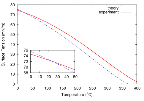
Figure 1: Comparison of Surface tension versus temperature for theoretical and experimental data. The experimental data is taken from NIST Lemmon et al. (2010). The length-scaling parameter $s_{d}$ is fit so that the theoretical surface tension will match the experimental surface tension near room temperature.

II.2 Association

The association free energy for our four-site model has the form:

$$F_{\text{assoc}}[n] =k_{B}T\int n_{\text{site}}(\textbf{r})\left(\ln X(\textbf{r})-\frac{X(\textbf{r})}{2}+\frac{1}{2}\right)d\textbf{r}$$ (4)

where $n_{\text{site}}(\textbf{r})$ is the density of bonding sites at position r:

$$n_{\text{site}}(\textbf{r}) =\begin{cases}4n(\textbf{r})&\text{this work}\\ 4n_{0}(\textbf{r})\zeta(\textbf{r})&\text{Hughes \emph{et al.}~{}\cite[cite]{\@@bibref{Authors Phrase1YearPhrase2}{hughes2013classical}{\@@citephrase{(}}{\@@citephrase{)}}}}\end{cases}$$ (5)

where the factor of four comes from the four hydrogen bond sites, the fundamental measure $n_{0}(\textbf{r})$ is the average density contacting point r, and $\zeta(\textbf{r})$ is a dimensionless measure of the density inhomogeneity from Yu and Wu Yu and Wu (2002). The functional $X(\textbf{r})$ is the fraction of association sites not hydrogen-bonded, which is determined for our 4-site model by the quadratic equation

$$X(\textbf{r}) =\frac{\sqrt{1+2n_{\text{site}}^{\prime}(\textbf{r})\kappa_{\textit{a}}g^{\textit{SW}}_{\sigma}(\textbf{r})\left(e^{-\beta\epsilon_{\textit{a}}}-1\right)}-1}{n_{\text{site}}^{\prime}(\textbf{r})\kappa_{\textit{a}}g^{\textit{SW}}_{\sigma}(\textbf{r})\left(e^{-\beta\epsilon_{\textit{a}}}-1\right)},$$ (6)

where

$$n_{\text{site}}^{\prime}(\textbf{r}) =\begin{cases}\frac{4}{\pi\sigma^{2}}\int n(\textbf{r}^{\prime})\delta(\sigma-|\textbf{r}-\textbf{r}^{\prime}|)d\textbf{r}^{\prime}&\text{this work}\\ 4n_{0}(\textbf{r})\zeta(\textbf{r})&\text{Hughes \emph{et al.}}\end{cases}$$ (7)

is the density of bonding sites that could bond to the sites $n_{\text{site}}(\textbf{r})$, and

$$g^{\textit{SW}}_{\sigma}(\textbf{r}) =g^{\textit{HS}}_{\sigma}(\textbf{r})+\frac{1}{4}\beta\left(\frac{\partial a_{1}}{\partial\eta_{\textit{d}}(\textbf{r})}-\frac{\lambda_{\textit{d}}}{3\eta_{\textit{d}}}\frac{\partial a_{1}}{\partial\lambda_{\textit{d}}}\right),$$ (8)

where $g^{\textit{HS}}_{\sigma}$ is the correlation function evaluated at contact for a hard-sphere fluid with a square-well dispersion potential, and $a_{1}$ and $a_{2}$ are the two terms in the dispersion free energy defined below Eq. 2. The radial distribution function of the square-well fluid $g^{\textit{SW}}_{\sigma}$ is written as a perturbative correction to the hard-sphere radial distribution function $g^{\textit{HS}}_{\sigma}$. The functional of Hughes et al. uses the $g_{\sigma}^{\textit{HS}}$ from Yu and Wu Yu and Wu (2002). In this work, we use the $g_{\sigma}^{\textit{HS}}$ derived by Schulte et al. Schulte et al. (2012).

As in Hughes et al., we use Clark’s five empirical parameters, and fit the calculated surface tension to experimental surface tension at ambient conditions by tuning the parameter $s_{d}$, which adjusts the length-scale of the average density used for the dispersion interaction. With the improved association term, we find these agree when $s_{d}$ is 0.454, which is an increase from the value of 0.353 found by Hughes et al.. In order to explore further the change made by the improved association term, we compared the new functional with that of Hughes et al. for the two hydrophobic cases of the hard rod and the hard spherical solute.

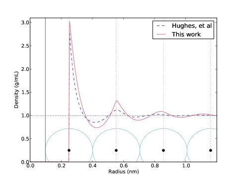
Figure 2: Density profiles for a water around a single hydrophobic rod of radius 0.1 nm. The solid red profile is from the functional developed in this paper and the dashed blue profile is the result from Hughes et al.. For scale, under the profiles is a cartoon of a string of hard spheres touching in one dimension. The horizontal black dotted line is the bulk density for water and the vertical line on the left at 0.1 nm represents the rod wall.

III Results

We will first discuss the case of a single hydrophobic rod immersed in water. Figure 2 shows the density profile of water near a rod with radius 1 Å. The density computed using the functional of this paper is qualitatively similar to that from Hughes et al., with a comparable density at contact—consistent with having made only a moderate change in the free energy. The first density peak near the surface is higher than that from Hughes et al., and the peak has a kink at the top. This reflects the improved accuracy of the $g_{\sigma}^{\textit{HS}}$ from Hughes et al., since beyond the first peak water molecules are unable to touch—or hydrogen bond to—molecules at the surface of the hard rod. This is illustrated under the profiles in Figure 2 by a cartoon of adjacent hard spheres that are increasingly distant from the hard rod surface.

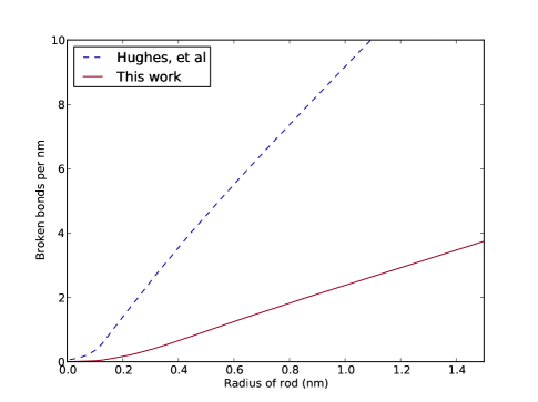
Figure 3: Broken hydrogen bonds per nanometer for hydrophobic rods immeresed in water. The solid red line uses the functional developed in this paper while the dashed blue line uses the functional from Hughes et al.. For large enough rods, the graph increases linearly for both functionals.

In addition to the density, we examine the number of hydrogen bonds which are broken due to the presence of a hard rod. We define this quantity as

$$N_{\text{broken HB}} =2\int(X(\textbf{r})-X_{\text{bulk}})n_{\text{site}}(\textbf{r})d\textbf{r}$$ (9)

where $X_{\text{bulk}}=0.13$ is the fraction of unbonded association sites in the bulk. The factor of 2 is chosen to account for the four association sites per molecule, and the fact that each broken hydrogen bond must be represented twice—once for each of the molecules involved. In Fig. 3 we show the number of hydrogen bonds broken by a hard rod per nanometer length, as predicted by the functional of Hughes et al. (dashed line) and this work (solid line), as a function of the radius of the hard rod. In each case in the limit of large rods, the number of broken bonds is proportional to the surface area. At every radius, the functional of Hughes et al. predicts approximately four times as many broken hydrogen bonds as the improved functional.

A common test case for studying hydrophobic solutes in water is the hard-sphere solute. Figure 4 shows results for the number of broken hydrogen bonds caused by a hard-sphere solute, as a function of the solute radius. As in Fig. 3, the number of broken bonds scales with surface area for large solutes, and the number of broken bonds is about four times smaller than the number from the functional of Hughes et al.. For solutes smaller than 3 Å in radius, there is less than a tenth of a hydrogen bond broken. This is consistent with the well-known fact that small solutes (unlike large solutes) do not disrupt the hydrogen-bonding network of water Chandler (2005).

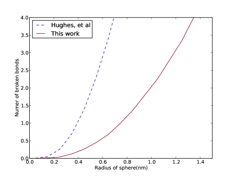
Figure 4: Broken hydrogen bonds for hard spheres immeresed in water. The solid red line uses our the functional developd in this paper while the dashed blue line is from Hughes et al..

IV Conclusion

We have modified the classical DFT for water developed by Hughes et al. Hughes et al. (2013) with the more accurate radial distribution function at contact developed by Schulte et al. Schulte et al. (2012), which affects the predicted hydrogen bonding between water molecules. We found that while this modification has a relatively mild effect on the free energy and density profiles, it predicts fewer broken hydrogen bonds around hydrophobic solutes and at aqueous interfaces.

References

- Jeanmairet et al. (2013) G. Jeanmairet, M. Levesque, R. Vuilleumier, and D. Borgis, The Journal of Physical Chemistry Letters 4, 619 (2013).
- Zhao et al. (2011a) S. Zhao, R. Ramirez, R. Vuilleumier, and D. Borgis, The Journal of chemical physics 134, 194102 (2011a).
- Zhao et al. (2011b) S. Zhao, Z. Jin, and J. Wu, The Journal of Physical Chemistry B 115, 6971 (2011b).
- Ramirez et al. (2005) R. Ramirez, M. Mareschal, and D. Borgis, Chemical physics 319, 261 (2005).
- Ramirez and Borgis (2005) R. Ramirez and D. Borgis, The Journal of Physical Chemistry B 109, 6754 (2005).
- Levesque et al. (2012a) M. Levesque, V. Marry, B. Rotenberg, G. Jeanmairet, R. Vuilleumier, and D. Borgis, The Journal of chemical physics 137, 224107 (2012a).
- Levesque et al. (2012b) M. Levesque, R. Vuilleumier, and D. Borgis, The Journal of Chemical Physics 137, 034115 (2012b).
- Lischner and Arias (2010) J. Lischner and T. Arias, The Journal of Physical Chemistry B 114, 1946 (2010).
- Hughes et al. (2013) J. Hughes, E. J. Krebs, D. Roundy, et al., The Journal of chemical physics 138, 024509 (2013).
- Clark et al. (2006) G. Clark, A. Haslam, A. Galindo, and G. Jackson, Molecular physics 104, 3561 (2006).
- Gloor et al. (2002) G. Gloor, F. Blas, E. del Rio, E. de Miguel, and G. Jackson, Fluid phase equilibria 194, 521 (2002).
- Gloor et al. (2004) G. Gloor, G. Jackson, F. Blas, E. Del Río, and E. de Miguel, The Journal of chemical physics 121, 12740 (2004).
- Gloor et al. (2007) G. Gloor, G. Jackson, F. Blas, E. del Río, and E. de Miguel, The Journal of Physical Chemistry C 111, 15513 (2007).
- Jaqaman et al. (2004) K. Jaqaman, K. Tuncay, and P. J. Ortoleva, J. Chem. Phys. 120, 926 (2004).
- Chuev and Sokolov (2006) G. N. Chuev and V. F. Sokolov, Journal of Physical Chemistry B 110, 18496 (2006).
- Fu and Wu (2005) D. Fu and J. Wu, Ind. Eng. Chem. Res 44, 1120 (2005).
- Kiselev and Ely (2006) S. Kiselev and J. Ely, Chemical Engineering Science 61, 5107 (2006).
- Blas et al. (2001) F. Blas, E. Del Río, E. De Miguel, and G. Jackson, Molecular Physics 99, 1851 (2001).
- Sundararaman et al. (2012) R. Sundararaman, K. Letchworth-Weaver, and T. A. Arias, The Journal of chemical physics 137, 044107 (2012).
- Chapman et al. (1989) W. Chapman, K. Gubbins, G. Jackson, and M. Radosz, Fluid Phase Equilibria 52, 31 (1989).
- Müller and Gubbins (2001) E. A. Müller and K. E. Gubbins, Industrial & engineering chemistry research 40, 2193 (2001).
- Tan et al. (2008) S. P. Tan, H. Adidharma, and M. Radosz, Industrial & Engineering Chemistry Research 47, 8063 (2008).
- Wertheim (1984a) M. S. Wertheim, Journal of statistical physics 35, 19 (1984a).
- Wertheim (1984b) M. S. Wertheim, Journal of statistical physics 35, 35 (1984b).
- Wertheim (1986a) M. S. Wertheim, Journal of statistical physics 42, 459 (1986a).
- Wertheim (1986b) M. S. Wertheim, Journal of statistical physics 42, 477 (1986b).
- Schulte et al. (2012) J. B. Schulte, P. A. Kreitzberg, C. V. Haglund, and D. Roundy, Physical Review E 86, 061201 (2012).
- Yu and Wu (2002) Y. X. Yu and J. Wu, The Journal of Chemical Physics 116, 7094 (2002).
- Gross (2009) J. Gross, The Journal of chemical physics 131, 204705 (2009).
- Roth et al. (2002) R. Roth, R. Evans, A. Lang, and G. Kahl, Journal of Physics: Condensed Matter 14, 12063 (2002).
- Gil-Villegas et al. (1997) A. Gil-Villegas, A. Galindo, P. Whitehead, S. Mills, G. Jackson, and A. Burgess, The Journal of Chemical Physics 106, 4168 (1997).
- Barker and Henderson (1976) J. Barker and D. Henderson, Reviews of Modern Physics 48, 587 (1976).
- Lemmon et al. (2010) E. W. Lemmon, M. O. McLinden, and D. G. Friend, “Nist chemistry webbook, nist standard reference database number 69,” (National Institute of Standards and Technology, Gaithersburg MD, 20899, 2010) Chap. Thermophysical Properties of Fluid Systems, http://webbook.nist.gov, (retrieved December 15, 2010).
- Chandler (2005) D. Chandler, Nature 437, 640 (2005).