Investment under uncertainty, competition and regulation

Abstract

We investigate a randomization procedure undertaken in real option games which can serve as a basic model of regulation in a duopoly model of preemptive investment. We recall the rigorous framework of M. Grasselli, V. Leclère and M. Ludkovsky (Priority Option: the value of being a leader, International Journal of Theoretical and Applied Finance, 16, 2013), and extend it to a random regulator. This model generalizes and unifies the different competitive frameworks proposed in the literature, and creates a new one similar to a Stackelberg leadership. We fully characterize strategic interactions in the several situations following from the parametrization of the regulator. Finally, we study the effect of the coordination game and uncertainty of outcome when agents are risk-averse, providing new intuitions for the standard case.

1 Introduction

A significant progress on the net present valuation method has been made by real option theory for new investment valuation. The latter uses recent methods from stochastic finance to price uncertainty and competition in complex investment situations. Real option games are the part of this theory dedicated to the competitive dimension. Following the seminal work of Smets [12], they correspond to an extensively studied situation, where two or more economic agents face with time a common project to invest into, and where there might be an advantage of being a leader (preemptive game) or a follower (attrition game). Grenadier [8], Paxson and Pinto [11] or Weeds [16] among many others develop nice examples of this type of model. On these problems and the related literature, Azevedo and Paxson [1] or Chevalier-Roignant et al. [5] provide comprehensive reviews. Real option games are especially dedicated to new investment opportunities following R&D developments, like technological products, a new drug or even real estate projects. The later investment opportunities indeed add competition risk to the uncertainty of future revenues in the strategic behavior of investors. The regulatory dimension is also an important part of such investment projects, and the present paper attempts to contribute in this direction.

The economic situation can be the following. We consider an investment opportunity on a new market for an homogeneous good, available for two agents labeled one and two. This investment opportunity is not constrained in time, but the corresponding market is regulated by an outside agent. Both agents have the same model for the project’s revenues, and both have also access to a financial market with one risky asset (a market portfolio) and a risk-free asset (a bank account). The situation is a non-cooperative duopoly of preemptive timing game for a single investment oppotunity.

A simple approach to regulation is to consider that when an agent wants to take advantage of such an opportunity, he must satisfy some non-financial criteria which are scrutinized by the regulator. Even though a model of regulatory decision is at the heart of this matter, we will take the most simple and naive approach. We will just assume that the regulator can accept or refuse an agent to proceed into the investment project, and that this decision is taken randomly. This extremely simple model finds its root in a widespread convenient assumption. In the standard real option game representing a Stackelberg duopoly, the settlement of leadership and followership is decided via the flipping of an even coin, independent of the model. The procedure is used for example in Weeds [16], Tsekeros [13] or Paxson and Pinto [11] who all refer to Grenadier [8] for the justification, which appears in a footnote for a real estate investment project:

A potential rationale for this assumption is that development requires approval from the local government. Approval may depend on who is first in line or arbitrary considerations.

This justification opens the door to many alterations of this assumption, inspired from other similar economic situations: the aforementioned considerations might lead to favor one competitor on the other or lead to a different outcome.

Let us take a brief moment to describe one of those economic situations we have in mind. Assume that two economic agents are running for the investment in a project with possibility of simultaneous investment, as in Grasselli et al. [7]. In practice, even if they are accurately described as symmetrical, they would never act at the exact same time, providing that instantaneous action in a continuous time model is just an idealized situation. Instead, they show their intention to invest to a third party (a regulator, a public institution) at approximatively the same time. An answer to a call for tenders is a typical example of such interactions. Then the arbitrator is invoked to judge the validity of these intentions. For example, he can evaluate which agent is the most suitable to be granted the project as a leader regarding qualitative criteria. This situation might be illustrated in particular where environmental or health exigences are in line. When simultaneous investment is impossible, the real estate market example of Grenadier [8] can also be cited again bearing in mind that, in addition to safety constraints, an aesthetic or confidence indicator can intervene in the decision of a market regulator. Because these criteria can be numerous, an approach via randomness of the decision is a decent first approximation. In the extremal case, the arbitrator can be biaised and show his preference for on agent. In general, it leads to an asymmetry in the chance to be elected leader and an unhedgeable risk, and perfectly informed agents should take into account this fact into their decision to invest or to defer. Those are some of the situations the introduction of a random regulator can shed some light on.

Our model is presented in a very particular way by using a normal form game in an extended natural virtual time, as initially proposed by Fudenberg and Tirole [6], and followed by Thijssen and al. [15] or Grasselli and al. [7]. This model bears a very specific interpretation, but appears to encompass in a continuous manner the Cournot competition setting of Smets [12] and the Stackelberg competition of Grenadier [8]. The introduction of a regulator also renders the market incomplete. We then follow two classical approaches, namely the risk-neutral and the risk-averse cases respectively. The latter case actually brings up new insights on the strategic interactions of players in the Cournot and Stackelberg setttings. Against the existing literature, the present contribution situates itself as a contribution to mathematical clarifications of the standard real option game, with new angles.

Let us present how the remaining of the paper proceeds. Section 2 introduces the standard model and its extension to the random regulatory framework. Section 3 provides the study of the model and optimal strategies in the general case. In Section 4, we present how the proposed model encompasses the usual types of competition, and propose a new asymmetrical situation related to the Stackelberg competition framework. Section 5 introduces risk-aversion in agents evaluation to study the effect of a random regulator and the uncertain outcome of a coordination game on equilibrium strategies of two opponents. Section 6 finishes on critism and possible extentions.

2 The model

2.1 The investment opportunity

We assume for the moment that the regulator does not intervene. The framework is thus the standard one that one shall find for example in Grasselli et al. [7]. Notations and results of this section follow from the latter. The later research will then be cited repeatedly in the present article.

We consider a stochastic basis $(\Omega,\mathcal{F},\mathbb{F},\mathbb{P})$ where $\mathbb{F}:=(\mathcal{F}_{t})_{t\geq 0}$ is the filtration of a one-dimensional Brownian motion $(W_{t})_{t\geq 0}$, i.e., $\mathcal{F}_{t}:=\sigma\{W_{s},\ 0\leq s\leq t\}$. The project delivers for each involved agent a random continuous stream of cash-flows $(D_{Q(t)}Y_{t})_{t\geq 0}$. Here, $Y_{t}$ is the stochastic profit per unit sold and $D_{Q(t)}$ is the quantity of sold units per agent actively involved on the market, when $Q(t)$ agents are actively participating at time $t$. The increments of $(Q(t))_{t\geq 0}$ inform on the timing decision of agents, and considering a perfect information setting, we assume that $(Q(t))_{t\geq 0}$ is a $\mathbb{F}$-adapted right-continuous process: agents are informed of competitors entry in the market, and expected future cash-flows can be computed. It is natural to assume that being alone in the market is better than sharing it with a competitor:

$$0=:D_{0}<D_{2}<D_{1}\;,$$ (1)

but we also assume these quantities to be known and constant. The process $(Y_{t})_{t\geq 0}$ is $\mathbb{F}$-adapted, non negative and continuous with dynamics given by

$$dY_{t}=Y_{t}(\nu dt+\eta dW_{t}),\quad t\geq 0\;,$$ (2)

with $(\nu,\eta)\in\mathbb{R}\times\mathbb{R}_{+}^{*}$. We assume that $(Y_{t})_{t\geq 0}$ is perfectly correlated to a liquid traded asset whose price dynamics is given by

$$dP_{t}=P_{t}(\mu dt+\sigma dW_{t})=P_{t}(rdt+\sigma dW^{\mathbb{Q}}_{t})$$ (3)

where $(\mu,\sigma)\in\mathbb{R}\times\mathbb{R}_{+}^{*}$, $r$ is the constant interest rate of the risk-free bank account available for both agents, and $W^{\mathbb{Q}}_{t}=W_{t}+\lambda t$ is a Brownian motion under the unique risk-neutral measure $\mathbb{Q}\sim\mathbb{P}$ of the arbitrage-free market. The variable $\lambda:=(\mu-r)/\sigma$ in 3 is the Sharpe ratio. The present financial setting is thus the standard Black-Scholes-Merton model [2] of a complete perfect financial market.

Remark 1.

The above setting defines $Y_{t}$ as a random unitary profit and $D$ as a fixed quantity, whereas Grenadier [9] and Grasselli et al.[7] labelled $Y_{t}$ and $D$ as the demand and the inverse demand curve respectively. This model choice has no incidence in complete market and Sections 2.2 and 2.3 herefater. The choice will be discussed in Remark 3 regarding the introduction of the regulator in Section 2.4.

2.2 The follower’s problem

In this setting, since $D_{Q(t)}$ takes known values, the future stream of cash-flows can be evaluated under the risk-neutral measure under which

$$dY_{t}=Y_{t}((\nu-\eta\lambda)dt+\eta dW^{\mathbb{Q}})\;.$$ (4)

Assume that one of the two agents, say agent one, desires to invest at time $t$ when $Y_{t}=y$. If $Q(t)=1$, then the available market for agent one is $D_{2}$. The risk-neutral expectation of the project’s discounted cash flows are then given by

$$V^{F}(t,y):=\mathbb{E}^{\mathbb{Q}}\left[\int_{t}^{\infty}e^{-r(s-t)}D_{2}Y_{s}ds\right]=\frac{D_{2}y}{\eta\lambda-(\nu-r)}=\frac{D_{2}y}{\delta}$$ (5)

with $\delta:=\eta\lambda-(\nu-r)$. We assume from now on $\delta>0$. Now to price the investment option of a follower, we recall that agent one can wait to invest as long as he wants. We also recall the sunk cost $K$ at time $\tau$ he invests. In the financial literature, this is interpreted as a Perpetual American call option of payoff $(D_{2}Y_{\tau}/\delta-K)^{+}$. The value function of this option is given by

$$F(t,y):=\sup\limits_{\tau\in\mathcal{T}_{t}}\mathbb{E}^{\mathbb{Q}}\left[e^{-r(\tau-t)}\left(\frac{D_{2}Y_{\tau}}{\delta}-K\right)^{+}\mathds{1}_{\{\tau<+\infty\}}|\mathcal{F}_{t}\right]$$ (6)

where $\mathcal{T}_{t}$ denotes the collection of all $\mathbb{F}$-stopping times with values in $[t,\infty]$. The solution to 6 is well-known in the literature, see Huang and Li [10] and Grenadier [8]. A formal recent proof can be found in Grasselli et al. [7].

Proposition 1 (Prop.1, [7]).

The solution to 6 is given by

$$F(y)=\left\{\begin{array}[]{ll}\frac{K}{\beta-1}\left(\frac{y}{Y_{F}}\right)^{\beta}&\text{ if }y\leq Y_{F},\\ \frac{D_{2}y}{\delta}-K&\text{ if }y>Y_{F},\\ \end{array}\right.$$ (7)

with a threshold $Y_{F}$ given by

$$Y_{F}:=\frac{\delta K\beta}{D_{2}(\beta-1)}$$ (8)

and

$$\beta:=\left(\frac{1}{2}-\frac{r-\delta}{\eta^{2}}\right)+\sqrt{\left(\frac{1}{2}-\frac{r-\delta}{\eta^{2}}\right)^{2}+\frac{2r}{\eta^{2}}}>1.$$ (9)

The behavior of the follower is thus quite explicit. He will defer investment until the demand reaches at least the level $Y_{F}=\beta/(\beta-1)K>K$ which depends on the profitability of the investment opportunity, the latter being conditioned by $\delta>0$. We thus introduce

$$\tau_{F}:=\tau(Y_{F})=\inf\{t\geq 0~{}:~{}Y_{t}\geq Y_{F}\}\;.$$ (10)

2.3 The leader’s problem

Assume now that instead of having $Q(t)=1$ we have $Q(t)=0$. Agent one investing at time $t$ will receive a stream of cash-flows associated to the level $D_{1}$ for some time, but he expects agent two to enter the market when the threshold $Y_{F}$ is triggered. After the moment $\tau_{F}$, both agents share the market and agent one receives cash-flows determined by level $D_{2}$. The project value is thus

$$V^{L}(t,y) :=\mathbb{E}^{\mathbb{Q}}\left[\int_{t}^{\infty}e^{-r(s-t)}(D_{1}\mathds{1}_{\{s<\tau_{F}\}}+D_{2}\mathds{1}_{\{s\geq\tau_{F}\}})Y_{s}^{t,y}ds\right]$$

$$=\frac{D_{1}y}{\delta}-\frac{(D_{1}-D_{2})Y_{F}}{\delta}\left(\frac{y}{Y_{F}}\right)^{\beta}$$

where detailed computation can be found in Grasselli et al. [7]. This allows to characterize the leader’s value function $L(t,y)$, i.e., the option to invest at time $t$ for a demand $y$, as well as the value of the project $S(t,y)$ in the situation of simultaneous investment.

Proposition 2 (Prop. 2, [7]).

The value function of a leader is given by

$$L(y)=\left\{\begin{array}[]{ll}\frac{D_{1}y}{\delta}-\frac{(D_{1}-D_{2})}{D_{2}}\frac{K\beta}{\beta-1}\left(\frac{y}{Y_{F}}\right)^{\beta}&\text{ if }y<Y_{F},\\ \frac{D_{2}y}{\delta}-K&\text{ if }y\geq Y_{F},\\ \end{array}\right.$$ (11)

If both agents invest simultaneously, we have

$$S(y):=\frac{D_{2}y}{\delta}-K\;.$$ (12)

Remark 2.

Notice that no exercise time is involved as we consider the interest of exercising immediately, $Y$ being non-negative. Notice also that $L$, $F$ and $S$ do not depend on $t$, since the problem is stationary.

The payoff of the investment opportunity is then fully characterized for any situation in the case of no regulatory intervention.

2.4 The regulator

Let us define $\tau_{1}$ and $\tau_{2}$ the time at which agents one and two respectively express their desire to invest. In full generality, $\tau_{i}$ for $i=1,2$ can depend on a probability of acting in a game, see the next subsection. We assume that agents cannot predict the decision of the regulator, so that $\tau_{1},\tau_{2}$ are $\mathbb{F}$-adapted stopping times. The regulator only intervenes at such times. If at time $\tau_{i}$ for $i=1,2$, $Q(\tau_{i}^{-})=0$, but $Q(\tau_{i})=1$ then his decision affects only agent $i$ who expresses his desire to be a leader. If however $Q(\tau_{i})=2$, then $\tau_{1}=\tau_{2}$ and the regulator shall decide if one or the other agent is accepted, none is or both are. Finally, if $Q(\tau_{i}^{-})=1$, then the regulator takes his decision upon the follower’s fate. The regulator decision thus depends on $\mathbb{F}$.

We introduce a probability space $(\Lambda,\mathcal{P}(\Lambda),\mathbb{A})$ where $\Lambda=\{\alpha_{0},\alpha_{1},\alpha_{2},\alpha_{S}\}$. We then introduce the product space $(\Omega\times\Lambda,\mathcal{F}\times\mathcal{P}(\Lambda),\mathbb{P}^{+})$ and the augmented filtration $\mathbb{F}^{+}:=(\mathcal{F}^{+}_{t})_{t\geq 0}$ with $\mathcal{F}^{+}_{t}:=\sigma\{\mathcal{F}_{t},\mathcal{P}(\Lambda)\}$. The regulator is modeled by a $\mathbb{F}^{+}$-adapted process.

Definition 2.1.

Fix $t$ and $Y_{t}=y$. For $i=1,2$, if $j=3-i$ is the index of the opponent and $\tau_{j}$ his time of investment, then agent $i$ desiring to invest at time $t$ receives

$$R_{i}(t,y):=\left\{\begin{array}[]{ll}0&\text{if }\alpha=\alpha_{0}\\ L(y)\mathds{1}_{\{t\leq\tau_{j}\}}+F(y)\mathds{1}_{\{t>\tau_{j}\}}&\text{if }\alpha=\alpha_{i}\\ F(y)\mathds{1}_{\{t=\tau_{j}\}}&\text{if }\alpha=\alpha_{j}\\ L(y)\mathds{1}_{\{t<\tau_{j}\}}+S(y)\mathds{1}_{\{t=\tau_{j}\}}+F(y)\mathds{1}_{\{t>\tau_{j}\}}&\text{if }\alpha=\alpha_{S}\\ \end{array}\right.\;.$$ (13)

Let us discuss briefly this representation. According to 13, agent $i$ is accepted if alternative $\alpha_{i}$ or $\alpha_{S}$ is picked up, and denied if $\alpha_{0}$ or $\alpha_{j}$ is picked up. It is therefore implicit in the model that time does not affect the regulator’s decision upon acceptability. However $Q(t)$ affects the position of leader or follower. Probability $\mathbb{P}^{+}$ can thus be given by $\mathbb{P}\times\mathbb{A}$, and probability $\mathbb{A}$ given by a quartet $\{q_{0},q_{1},q_{2},q_{S}\}$. However, as we will see shortly, the alternative $\alpha_{0}$ is irrelevant in what follows due to the way regulatory intevention is modelled. We assume $q_{0}<1$. Since for the unregulated model we assumed that agents are symmetrical, the general study of the regulator’s parameters given by $\mathbb{A}$ will be chosen without loss of generality such that $q_{1}\geq q_{2}$.

An additional major change comes into the evaluation of payoffs. Agents information is reduced to $\mathbb{F}$. Therefore the final settlement is not evaluable as in the complete market setting, and we shall introduce a pricing criterion. We follow Smets [12], Grenadier [8] and many others by making the usual assumption that agents are risk-neutral, i.e., they evaluate the payoffs by taking the expectation of previously computed values under $\mathbb{A}$. The incomplete market is also commonly handled via utility maximization, see Benssoussan et al. [3] and Grasselli et al. [7]. We postpone this approach to Section 5.

Remark 3.

Expectations of 13 are made under the minimal entropy martingale measure $\mathbb{Q}\times\mathbb{A}$ for this problem, meaning that uncertainty of the model follows a semi-complete market hypothesis: if we reduce uncertainty to the market information $\mathbb{F}$, then the market is complete. See Becherer [4] for details. Recalling Remark 1, we can thus highligh that payoffs $L(y)$, $F(y)$ or $S(y)$ can be perfectectly evaluated. Therefore definitions of $Y$ and $D$ only matter in the interpretation of the model and the present choice of probability is not affected by such interpretation.

Once the outcome of $\Lambda$ is settled, the payoff then depends on $Q(t)$, i.e., $\tau_{j}$. We thus focus now on strategic interactions that determine $Q(t)$.

2.5 Timing strategies

It has been observed since Fudenberg & Tirole [6] that real time $t\geq 0$ is not sufficient to describe strategic possibilities of opponents in a coordination game. If $Q(t)=0$ and agents coordinate by deciding to invest with probabilities $p_{i}\in(0,1)$ for $i=1,2$, then a one-round game at time $t$ implies a probability $(1-p_{1})(1-p_{2})$ to exit without at least one investor. However, another coordination situation appears for the instant just after and the game shall be repeated with the same parameters. The problem has been settled by Fudenberg and Tirole [6] in the deterministic case, and recently by Thijssen et al. [15] for the stochastic setting. We extend it to the model with regulator in the following manner.

It consists in extending time $t\in\mathbb{R}_{+}$ to $(t,k,l)\in\mathbb{R}_{+}\times\mathbb{N}^{*}\times\mathbb{N}^{*}$. The filtration $\mathbb{F}$ is augmented via $\mathcal{F}_{t,i,j}=\mathcal{F}_{t,k,l}\subseteq\mathcal{F}_{t^{\prime},i,j}$ for any $t<t^{\prime}$ and any $(i,j)\neq(k,l)$, and the state process is extended to $Y_{(t,k,l)}:=Y_{t}$. Therefore, when both agents desire to invest at the same time $t$, we extend the time line by freezing real time $t$ and indefinitely repeating a game on natural time $k$. Once the issue of the game is settled, the regulator intervenes on natural time $l=1$. If no participant is accepted, i.e., if $\alpha_{0}$ is picked up. the game is replayed for $l=2$, and so on.

This model needs to be commented. At first glance, a natural assumption is to make the regulator intervene once and for all for each agent or both at the same time. If the regulator refuses the entry of a competitor, one could assume for example that the game is over or that a delay is imposed before any other action of the rejected agent. The time extention above and the following Definition 2.2 do not obey this rule. However, it can be related to a unique intervention of the regulator by forthcoming Corollary 1 and Proposition 4, see Remark 4 at the end of Section 3.1. The motivation for the present model lies in presentation details. In Definition 2.1, it allows the generic expression 13 and avoids direct conditioning of $R_{i}(t,y)$ on the position of agent $i$. Expression 13 can thus be directly handled and modified to represent a more realistic situation than one implying the systematic entry of at least one player, as it will be shown in the next section. The present model also allows for the relevant specific cases of Section 4.1 and Section 4.2. By using the framework of Fudenberg and Tirole [6], the present model also shows its limitations as an idealized situation.

Definition 2.2.

A strategy for agent $i\in\{1,2\}$ is defined as a pair of $\mathbb{F}$-adapted processes $(G^{i}_{(t,k,l)},p^{i}_{(t,k,l)})$ taking values in $[0,1]^{2}$ such that

1. The process $G^{i}_{(t,k,l)}$ is of the type $G^{i}_{(t,k,l)}(Y_{t})=G^{i}_{t}(Y_{t})=\mathds{1}_{\{t\geq\tau(\hat{y})\}}$ with $\tau(\hat{y}):=\inf\{t\geq 0~{}:~{}Y_{t}\geq\hat{y}\}$.

2. The process $p_{i}(t,k,l)$ is of the type $p_{i}(t,k,l)=p_{i}(t)=p^{i}(Y_{t})$.

The reduced set of strategies is motivated by several facts. Since the process $Y$ is Markov, we can focus without loss of generality on Markov sub-game perfect equilibrium strategies. The process $G^{i}_{(t,k)}$ is a non-decreasing càdlàg process, and refers to the cumulative probability of agent $i$ exercising before $t$. Its use is kept when agent $i$ does not exercise immediately the option to invest, and when exercise depends on a specific stopping time of the form $\tau(\hat{Y})$, such as the follower strategy. The process $p^{i}_{(t,k,l)}$ denotes the probability of exercising in a coordinate game at round $k$, after $l-1$ denials of the regulator, when $\alpha=\alpha_{0}$. It should be stationary and not depend on the previous rounds of the game since no additional information is given. For both processes, the information is given by $\mathbb{F}$ and thus reduces to $Y_{t}$ at time $t$. Additional details can be found in Thijssen et al. [15].

3 Optimal behavior and Nash equilibria

3.1 Conditions for a coordination game

A first statement about payoffs can be immediately provided. A formal proof can be found in Grasselli et al. [7], following arguments initially developped in Grenadier [8, 9].

Proposition 3 (Prop. 1, [9]).

There exists a unique point $Y_{L}\in(0,Y_{F})$ such that

$$\left\{\begin{array}[]{ll}S(y)<L(y)<F(y)&\text{ for }y<Y_{L},\\ S(y)<L(y)=F(y)&\text{ for }y=Y_{L},\\ S(y)<F(y)<L(y)&\text{ for }Y_{L}<y<Y_{F},\\ S(y)=F(y)=L(y)&\text{ for }y\geq Y_{F}\;.\end{array}\right.$$ (14)

Fix $t$ and $Y_{t}=y$. In the deregulated situation, three different cases are thus possible, depending on the three intervals given by $0<Y_{L}<Y_{F}<+\infty$. It appears that in our framework, the discrimination also applies.

Consider the following situation. Assume $Q(t)=0$ and $t=\tau_{1}<\tau_{2}$: agent one wants to start investing in the project as a leader and agent two allows it, i.e., $(p_{1}(t),p_{2}(t))=(1,0)$. By looking at 13, agent one receives $L(y)$ with probability $q_{1}+q_{S}$ and $0$ with probability $q_{2}+q_{0}$. However, as noticed for the coordination game, if agent one is denied investment at $(t,1,1)$, he can try at $(t,1,2)$ and so on until he obtains $L(y)$. Consequently, if $q_{0}<1$ agents can do as if $\alpha_{0}$ is never picked up, see Remark 4 below. The setting is limited by the continuous time approach and Proposition 3 applies as well as in the standard case. The situation is identical if $\tau_{2}<\tau_{1}$.

Corollary 1.

Let $t\geq 0$ and $y>0$. Then for $i=1,2$

1. if $y<Y_{L}$, agent $i$ defers action until $\tau(Y_{L})$;

2. if $y>Y_{F}$, agent $i$ exercises immediately, i.e., $\tau_{i}=t$.

Proof.

(d) According to 14, if $\tau_{1}\neq\tau_{2}$, expected payoffs given to 13 verify $(q_{S}+q_{i})L(y)<(q_{S}+q_{i})F(y)$ and there is no incentive to act for agent $i$, $i=1,2$.

(e) Since $S(y)=F(y)=L(y)$ and $\tau_{F}=t$, both agents act with probability $(p_{1}(t),p_{2}(t))=(1,1)$. Since $q_{0}<1$, they submit their request as much as needed and receive $S(y)$ with probability $(1-q_{0})\sum_{l\in\mathbb{N}}q_{0}^{l}=1$. ∎

Corollary 1 does not describe which action is undertaken at $\tau(Y_{L})$ or if $y=Y_{F}$. We are thus left to study the case where $Y_{L}\leq y\leq Y_{F}$. This is done by considering a coordination game. Following the reasoning of the above proof, definition 13 allows to give the expected payoffs of the game. Let us define

$$(S_{1},S_{2}):=\left(\frac{1}{1-q_{0}}(q_{1}L+q_{2}F+q_{S}S),\frac{1}{1-q_{0}}(q_{2}L+q_{1}F+q_{S}S)\right)\;.$$ (15)

Notice that $S_{i}$ are bounded by $\max\{L,F,S\}$ since $q_{1}+q_{2}+q_{s}=1-q_{0}$.

Proposition 4.

For any $q_{0}<1$, agents play the coordination game given by Table 1 if $Y_{L}<y<Y_{F}$. Consequently, we can assume $q_{0}=0$ without loss of generality.

	Exercise	Defer
Exercise	$(S_{1}(y),S_{2}(y))$	$(L(y),F(y))$
Defer	$(F(y),L(y))$	Repeat

Table 1: Coordination game at $(t,k,l)$.

Proof.

If $\alpha=\alpha_{0}$ after settlement at round $k$ of the game, time goes from $(t,k,l)$ to $(t,1,l+1)$ and the game is repeated. Therefore, according to 13, the game takes the form of Table 1 for a fixed $l$ and is settled with probability $1-q_{0}$, or canceled and repeated with probability $q_{0}$. If $(p_{1},p_{2})$ is a given strategy for the game at $t$ and $(E_{1}(p_{1},p_{2}),E_{2}(p_{1},p_{2}))$ the consequent expected payoff for agents one and two in the game of Table 1, then the total expected payoff for agent $i$ at time $t$ is

$$E_{i}(p_{1},p_{2})(1-q_{0})\sum_{l\in\mathbb{N}}q_{0}^{l}=E_{i}(p_{1},p_{2})\;.$$ (16)

The game is thus not affected by $q_{0}<1$, which can take any value stricly lower than one. Without loss of generality, we can then take $q_{0}=0$ and reduce the game to one intervention of the regulator, i.e. $l\leq 1$.

When $\tau_{1}\neq\tau_{2}$, the probability that the regulator accepts agent $i$ demand for investment is $q_{i}+q_{S}$, see Corollary 1. There is a complete equivalence of payoffs and strategies for quartet $\{q_{0},q_{1},q_{2},q_{S}\}$ and quartet $\{0,q_{1}/(1-q_{0}),q_{2}/(1-q_{0}),q_{S}/(1-q_{0})\}$. Probability $q_{0}$ can then be settled to zero. ∎

Remark 4.

Extended time model of Section 2.5 implies strong limitations to the issues of the game: Corollary 1 and Proposition 4 impose the emergence of at least one player at $\tau_{1}$ and $\tau_{2}$. The confrontation has thus three outcomes and can bear the following interpretation. In the present model of competition, a regulator intervenes only if the two agents attemps to enter the investment opportunity at the same time. He then decides among three alternatives: letting one, or the other, or both agents enter the opportunity. The decision of the regulator is definitive and it is thus possible to connect this procedure to the original one of Grenadier [8] mentionned in the introduction, see also Section 4.1.

According to Remark 4, we settle $q_{0}=0$ from now on. We now turn to the solution to Table 1.

3.2 Solution in the regular case

We reduce the analysis here to the case where $0<q_{2}\leq q_{1}<1-q_{2}$. We can now assume that

$$\max(p_{1},p_{2})>0\;.$$ (17)

We now introduce $p_{0}(y):=(L(y)-F(y))/(L(y)-S(y))$ and two functions

$$P_{i}(y):=\frac{p_{0}(y)}{q_{i}p_{0}(y)+q_{S}}=\frac{L(y)-F(y)}{L(y)-S_{j}(y)},\quad i\neq j\in\{1,2\}^{2}\;.$$ (18)

The values of $P_{i}$ strongly discriminates the issue of the game. Since $q_{1}\geq q_{2}$, if $Y_{L}\leq y\leq Y_{F}$, then $S_{1}(y)\geq S_{2}(y)$ according to 14 on that interval and $P_{2}(y)\geq P_{1}(y)$.

Lemma 3.1.

The functions $P_{2}$ and $P_{1}$ are increasing on $[Y_{L},Y_{F}]$.

Proof.

By taking $d_{1}(y):=L(y)-F(y)$ and $d_{2}(y):=S(y)-F(y)$, we get

$$P_{i}(y)=\frac{1}{q_{i}}\left[\frac{d_{1}(y)}{d_{1}(y)+\gamma_{i}(d_{1}(y)-d_{2}(y))}\right]$$

and

$$P^{\prime}_{i}(y)=\frac{1}{q_{i}}\left[\frac{\gamma_{i}(d_{1}(y)d^{\prime}_{2}(y)-d_{2}(y)d^{\prime}_{1}(y))}{(d_{1}(y)+\gamma_{i}(d_{1}(y)-d_{2}(y)))^{2}}\right]$$

where $\gamma_{i}:=q_{S}/q_{i}\leq 1\text{ with }i\in\{1,2\}.$ We are thus interested in the sign of the quantity $g(y):=d_{1}(y)d^{\prime}_{2}(y)-d_{2}(y)d^{\prime}_{1}(y)$ which quickly leads to

$$\frac{g(y)\delta}{yD_{2}}=\left(\frac{y}{Y_{F}}\right)^{\beta-1}\left[(D_{1}-D_{2})(\beta+\frac{1}{\beta}-2-\frac{\delta K}{D_{2}})\right]+\frac{\delta K}{D_{2}}\left(D_{1}-D_{2}\right)\;.$$

Since $\beta>1$, $(y/Y_{F})^{\beta-1}$ is increasing in $y$. Since $0<y\leq Y_{F}$, it suffices to verify that $(\delta K)/D_{2}\geq(\beta+1/\beta-2-(\delta K)/D_{2})$, which is naturally the case for any $\beta$, to obtain that $g$ is non-negative on the interval. ∎

We will omit for now the symmetric case and assume $P_{1}(y)<P_{2}(y)$ for $Y_{L}<y<Y_{F}$. Recall now that $q_{i}>0$ for $i=1,2$. Then $P_{i}(Y_{F})=1/(q_{i}+q_{S})>1$ for $i=1,2$. Accordingly and by Lemma 3.1, there exists $Y_{L}<Y_{1}<Y_{2}<Y_{F}$ such that

$$\begin{array}[]{l}F(Y_{1})=q_{1}L(Y_{1})+q_{2}F(Y_{1})+q_{S}S(Y_{1})=S_{1}(Y_{1})\;,\\ F(Y_{2})=q_{2}L(Y_{2})+q_{1}F(Y_{2})+q_{S}S(Y_{2})=S_{2}(Y_{2})\;.\end{array}$$ (19)

Proposition 5.

Assume $Y_{L}<y<Y_{F}$. Then solutions of Table 1 are of three types:

1. If $Y_{L}<y<Y_{1}$ the game has three Nash Equilibria given by two pure strategies $(1,0)$ and $(1,0)$, and one mixed strategy $(P_{1}(y),P_{2}(y))$.

2. If $Y_{1}\leq 1<Y_{2}$, the game has one Nash Equilibrium given by strategies $(1,0)$.

3. If $Y_{2}\leq y<Y_{F}$, the game has one Nash Equilibrium given by strategies $(1,1)$.

Proof.

For $Y_{L}<y<Y_{1}$, we have $P_{1}<P_{2}<1$. Fix an arbitrary constant strategy $(p_{1},p_{2})\in[0,1]^{2}$. Considering the $\mathbb{A}$-expected payoffs, agent one receives $L(y)$ at the end of the game with a probability

$$a_{1}:=p_{1}\sum_{k\in\mathbb{N}^{*}}(1-p_{1})^{k-1}(1-p_{2})^{k}=\frac{p_{1}(1-p_{2})}{p_{1}+p_{2}-p_{1}p_{2}}\;.$$ (20)

Symmetrically, he receives $F(y)$, and agent two receives $L(y)$ with probability

$$a_{2}:=\dfrac{p_{2}(1-p_{1})}{p_{1}+p_{2}-p_{1}p_{2}}\;,$$ (21)

and they receives $(S_{1}(y),S_{2}(y))$ with probability

$$a_{S}:=\dfrac{p_{1}p_{2}}{p_{1}+p_{2}-p_{1}p_{2}}\;.$$ (22)

The expected payoff of the game for agent one is given by

$$\begin{array}[]{ll}E_{1}(p_{1},p_{2})&:=a_{1}L(y)+a_{2}F(y)+a_{S}S_{1}(y)\\ &\ =(a_{1}+a_{S}q_{1})L(y)+(a_{2}+a_{S}q_{2})F(y)+a_{S}q_{S}S(y)\;.\end{array}$$ (23)

A similar expression $E_{2}$ is given for agent two. Now fix $p_{2}$. Since $E_{1}$ is a continuous function of both variables, maximum of 23 depends on

$$\frac{\partial E_{1}}{\partial p_{1}}(p_{1},p_{2})=\frac{p_{2}(L(y)-F(y)+p_{2}^{2}(S_{1}(y)-L(y))}{(p_{1}(1-p_{2})+p_{2})^{2}}\;.$$ (24)

One can then see that the sign of 24 is the sign of $(p_{2}-P_{2})$. A similar discrimination for agent two implies $P_{1}$.

(a) If $Y_{L}<y<Y_{1}$, then according to 18 and 19, $P_{i}<1$ for $i=1,2$. Three situations emerge:

1. If $p_{2}>P_{2}$, the optimal $p_{1}$ is $0$. Then by 24, $E_{2}$ should not depend on $p_{2}$, and the situation is stable for any pair $(0,p_{2})$ with $p_{2}$ in $(P_{2},1]$.

2. If $p_{2}=P_{2}$, $E_{1}$ is constant and $p_{1}$ can take any value. If $p_{1}<P_{1}$, then by symmetry $p_{2}$ should take value $1$, leading to case (i). If $p_{1}=P_{1}$, $E_{2}$ is constant and either $p_{2}=P_{2}$, or we fall in case (i) or (iii). The only possible equilibrium is thus $(P_{1},P_{2})$.

3. If $p_{2}<P_{2}$, $E_{1}$ is increasing with $p_{1}$ and agent one shall play with probability $p_{1}=1>P_{1}$. Therefore $p_{2}$ optimizes $E_{2}$ when being $0$, and $E_{1}$ becomes independent of $p_{1}$. Altogether, situation stays unchanged if $p_{1}\in(P_{1},1]$ or if $p_{1}=0$. Otherwise, if $p_{1}\leq P_{1}$, we fall back into cases (i) or (ii). The equilibria here are $(p_{1},0)$ with $p_{1}\in(P_{1},1]$, and the trivial case $(0,0)$.

Recalling constraint 17, we get rid of case $(0,0)$. Coming back to the issue of the game when $k$ goes to infinity in $(t,k,1)$, three situations emerge from the above calculation. Two of them are pure coordinated equilibriums, of the type $(a_{1},a_{2})=(1,0)$ or $(0,1)$, which can be produced by pure coordinated strategies $(p_{1},p_{2})=(a_{1},a_{2})$, settling the game in only one round. The third one is a mixed equilibrium given by $(p_{1},p_{2}):=(P_{1},P_{2})$.

(b) According to 19, $S_{1}(Y_{1})=F(Y_{1})$. Following Lemma 3.1, agent one prefers being a leader for $y\geq Y_{1}$ and prefers a regulator intervention rather than the follower position, i.e. $S_{1}(y)\geq F(y)$. Thus $p_{1}=1$. For agent two, defering means receiving $F(y)>F(Y_{1})$ and exercising implies a regulation intervention. Since $y<Y_{2}$, $q_{1}F(y)+q_{2}L(y)+q_{S}S(y)<F(y)$ and defering is his best option: $p_{2}=0$. That means that on $(Y_{1},Y_{2})$, the equilibrium strategy is $(p_{1},p_{2})=(1,0)$.

(c) On the interval $[Y_{2},Y_{F})$, the reasoning of (b) still applies for agent one by monotony, and $p_{1}=1$. The second agent can finally bear the same uncertainty if $y\geq Y_{2}$, and $p_{2}=1$. Here, $1\leq P_{1}(y)\leq P_{2}(y)$ and both agents have greater expected payoff by letting the regulator intervene rather than being follower. Equilibrium exists when both agents exercise. ∎

Two reasons force us to prefer the strategy $(P_{1},P_{2})$ on $(1,0)$ and $(0,1)$ in case (a). First, it is the only one which extends naturally the symmetric case. Second, it is the only trembling-hand equilibrium. Considering $(P_{1},P_{2})$ in the interval (a), $(a_{1},a_{2},a_{S})$ follows according to 20, 21 and 22,

$$(a_{1},a_{2},a_{S})=\left(\frac{1-p_{0}}{2-p_{0}},\frac{1-p_{0}}{2-p_{0}},\frac{p_{0}}{2-p_{0}}\right)\;,$$ (25)

If we plug 25 into 23, we obtain that the payoff of respective agents do not depend on $(q_{1},q_{2},q_{S})$:

$$E_{1}(P_{1},P_{2})=E_{2}(P_{1},P_{2})=\frac{1-p_{0}}{2-p_{0}}(L(y)+F(y))+\frac{a_{0}}{2-p_{0}}S(y)\;.$$ (26)

In the case $q_{S}>0$, they are equal to $F$. As notice in Grasselli et al.[7], we retrieve a mathematical expression of the rent equalization principle of Fudenberg and Tirole [6]: agents are indifferent between playing the game and being the follower, and time value of leadership vanishes with preemption. In addition, asymmetry $q_{1}\geq q_{2}$ does not affect the payoffs and the final outcome of the game after decision of the regulator has the same probability as in the deregulated situation, see Grasselli et al. [7].

Figure 1: Values of $p_{1}(y)$ (blue) and $p_{2}(y)$ (red) for $(q_{1},q_{2},q_{S})=(0.5,0.2,0.3)$. Areas (a), (b) and (c) are separated by lines at $Y_{1}=0.53$ and $Y_{2}=0.72$ on $[Y_{L},Y_{F}]=[0.37,1.83]$. Area (d) is at the left of the graph and (e) at the right of it. Parameters set at $(K,\nu,\eta,\mu,\sigma,r,D_{1},D_{2})=(10,0.01,0.2,0.04,0.3,0.03,1,0.35)$.

3.2.1 Endpoints and overall strategy

We have to study junctions of areas (d) with (a), and (c) with (e). The technical issue has been settled in Thijssen et al. [15].

Lemma 3.2.

Assume $y=Y_{L}$. Then both agents have a probability $1/2$ to be leader or follower, and receive $L(Y_{L})=F(Y_{L})$.

Proof.

The junction of $[0,Y_{L})$ with $[Y_{L},Y_{1}]$ is a delicate point. At the left of point $Y_{L}$, no agent wants to invest. We thus shall use the strategy $G^{i}(Y_{L})$ for both agents. By right-continuity of this process, both agents shall exercise with probability 1 at point $Y_{L}$. Each agent receives $R_{i}(y)$ which takes value $L(y)=F(y)$ with probability $q_{1}+q_{2}$ and $S(y)$ with probability $q_{S}$:

$$E_{1}(y)=E_{2}(y)=(q_{1}+q_{2})F(y)+q_{S}S(y)\;.$$ (27)

At the right side of point $Y_{L}$ however, $P_{i}$ converges to $0$ when $y$ converges to $Y_{L}$, for $i=1,2$. Therefore, so do $(p_{1},p_{2})$ toward $(0,0)$. We cannot reconcile $G^{i}_{\tau(Y_{L})}(Y_{L})$ with $(p_{1}(Y_{L}),p_{2}(Y_{L}))=(0,0)$ and shall compare the payoffs. A short calculation provides

$$\lim_{y\downarrow Y_{L}}\frac{a_{1}(y)}{a_{2}(y)}=1\;\mbox{ and }\;\lim_{y\downarrow Y_{L}}a_{s}(y)=0\;.$$ (28)

Therefore at point $Y_{L}$, $(a_{1}(Y_{L}),a_{2}(Y_{L}),a_{S}(Y_{L}))=(1/2,1/2,0)$. It is clear at point $Y_{L}$ that the second option is better for both agents. ∎

Remark 5.

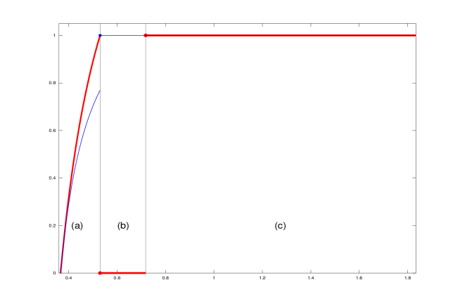
There is a continuity of behavior between (d) and (a) from the fact that regulatory intervention does not impact the outcome of the game, from the point of view of discrimination between the two agents: simultaneous investment is improbable at point $Y_{L}$, and probability $a_{S}(y)$ is continuous and null at this point. Consequently, the local behavior of agents around $Y_{L}$ is similar to the one given in Grasselli et al. [7]. Altogether and observing Figure 1, mixed strategies are right-continuous.

Let us complete the strategic interaction of the two agents by summarizing the previous results in the following Theorem. As we will see in the next section for singular cases, it extends Theorem 4 in [7].

Theorem 3.3.

Consider the strategic economic situation presented in Section 2, with

$$\min\{q_{1},q_{2},q_{S}\}>0\;\mbox{ and }\;q_{0}=0\;.$$ (29)

Then there exists a Markov sub-game perfect equilibrium with strategies depending on the level of profits as follows:

1. If $y<Y_{L}$, both agents wait for the profit level to rise and reach $Y_{L}$.

2. At $y=Y_{L}$, there is no simultaneous exercise and each agent has an equal probability of emerging as a leader while the other becomes a follower and waits until the profit level reaches $Y_{F}$.

3. If $Y_{L}<y<Y_{1}$, each agent choses a mixed strategy consisting of exercising the option to invest with probability $P_{i}(y)$. Their expected payoffs are equal, and the regulator intervenes on the settlement of positions.

4. If $Y_{1}\leq y<Y_{2}$, agent one exercises his option and agent two becomes a follower and waits until $y$ reaches $Y_{F}$.

5. If $Y_{2}\leq y<Y_{F}$, both agents express their desire to invest immediately, and the regulator is called. If one agent is elected leader, the other one becomes follower and waits until $y$ reaches $Y_{F}$.

6. If $Y_{F}\geq y$, both agents act as in (v), but if a follower emerges, he invest immediately after the other agent.

Some comments are in order. First, we shall emphasize that the regulator theoretically intervenes for any situation where $y\geq Y_{L}$. However, as explained at the beginning of this section, its intervention becomes mostly irrelevant in continuous time when agents do not act simultaneously. Its impact is unavoidable to settle the final payoff after the game, but its influence on agents’ strategies boils down to the interval $(Y_{L},Y_{2}]$.

At point $Y_{1}$, there is a strong discontinuity in the optimal behavior of both agents. For $y<Y_{1}$, the mixed strategy used by agent two tends toward a pure strategy with systematic investment. However at the point itself, the second agent defers investment and becomes the follower. It follows from the fact that agent one is indifferent between being follower or letting the regulator decide the outcome at this point. He suddenly seeks, without hesitation, for the leader’s position, creating a discontinuity in his behavior. The same happens for agent two at $Y_{2}$, creating another discontinuity in the strategy of the latter.

4 Singular cases

The proposed framework encompasses in a natural way the two main competition situations encountered in the literature, namely the Cournot competition and the Stackelberg competition. By introducing minor changes in the regulatory intervention, it is also possible to represent the situation of Stackelberg leadership advantage. Finally, our setting allows to study a new and weaker type of advantage we call weak Stackelberg leadership.

4.1 The Cournot and Stackelberg competitions

The Cournot duopoly refers to a situation when both players adjust quantities simultaneously. This is the framework of Grasseli et al. [7], involving the payoff $S(y)$ if agents invest at the same time. Recalling Definition 2.1, this framework corresponds to

$$(q_{1},q_{2},q_{S})=(0,0,1)\;.$$ (30)

We notice that agents then become symmetrical. This appears from 18 which implies $P_{1}(y)=P_{2}(y)=p_{0}(y)$. Additionally, $p_{0}(y)\in(0,1)$ if $y\in(Y_{L},Y_{F})$, and is increasing on this interval according to Lemma 3.

The Stackelberg competition refers to a situation where competitors adjust the level $D_{Q(t)}$ sequentially. In a preemptive game, this implies that in the case of simultaneous investment, one agent is elected leader and the other one becomes follower. This setting implies an exogenous randomization procedure, which by symmetry is given by a flipping of a fair coin. The procedure is described as such in Grenadier [8], Weeds [16], Tsekeros [13] or Paxson and Pinto [11]. Recalling Definition 2.1, the setting is retrieved by fixing

$$(q_{1},q_{2},q_{S})=(1/2,1/2,0)\;.$$ (31)

The implication in our context is the following: by symmetry, $P_{1}(y)=P_{2}(y)=2$. Therefore, the interval $(Y_{L},Y_{2})$ reduces to nothing, i.e., $Y_{L}=Y_{1}=Y_{2}$, and the strategical behavior boils down to (i), (v) and (vi) in Theorem 3.3.

Remark 6.

Notice that any combination $q_{2}=1-q_{1}\in(0,1)$ provides the same result as in 31, as $P_{i}(y)=1/q_{i}>1$ for $i=1,2$. The strategic behavior is unchanged with an unfair coin flipping. This is foreseeable as $q_{i}L(y)+(1-q_{i})F(y)>F(y)$ on $(Y_{L},Y_{F})$. This will also hold for a convex combination, i.e., for risk-averse agents.

Remark 7.

Assume now symmetry in the initial framework, i.e., $q:=q_{1}=q_{2}\in(0,1/2)$. We have $Y_{S}:=Y_{1}=Y_{2}$, and the region (b) reduces to nothing. By recalling 19, we straightly obtain

$$\lim\limits_{q\uparrow 1/2}Y_{S}=Y_{L}\ \;\mbox{ and }\;\ \lim\limits_{q\downarrow 0}Y_{S}=Y_{F}\;.$$ (32)

Therefore, the regulation intervention encompasses in a continuous manner the two usual types of games described above.

4.2 Stackelberg leadership

This economic situation represents an asymmetrical competition where the roles of leader and follower are predetermined exogenously. It can be justified as in Bensoussan et al. [3] by regulatory or competitive advantage. However Definition 2.1 does not allow to retrieve this case directly. Instead, we can extend it by conditioning the probability quartet $\{q_{0},q_{1},q_{2},q_{S}\}$. In this situation, the probability $\mathbb{P}^{+}$ depends on $\mathbb{F}$-adapted events in the following manner:

$$\mathbb{P}^{+}(\alpha_{0}|t<\tau_{1})=1\;\mbox{ and }\;\mathbb{P}^{+}(\alpha_{1}|t\geq\tau_{1})=1\;.$$ (33)

This means that no investment is allowed until agent one decides to invest, which leads automatically to the leader position. The strategical interaction is then pretty different from the endogenous attribution of roles. See Grasselli and al.[7] for a comparison of this situation with the Cournot game.

4.3 The weak Stackelberg advantage

We propose here a different type of competitive situation. Consider the investment timing problem in a duopoly where agent one has, as in the Stackelberg leadership, a significant advantage due to exogenous qualities. We assume that for particular reasons, the regulator only allows one agent at a time to invest in the shared opportunity. The advantage of agent one thus translates into a preference of the regulator, but only in the case of simultaneous move of the two agents. That means that agent two can still, in theory, preempt agent one. This situation can be covered by simply setting

$$(q_{1},q_{2},q_{S})=(1,0,0)\;.$$ (34)

In this setting, the results of Section 3 apply without loss of generality.

Proposition 6.

Assume 34. Then the optimal strategy for agents one and two is given by $(G^{1}(Y_{L}),G^{2}(Y_{F}))$.

Proof.

It suffices to consider the game of Table 1 on the interval $[Y_{L},Y_{F})$. The Nash equilibrium is given by $(p_{1}(y),p_{2}(y))=(1,0)$ for any $y\in[Y_{L},Y_{F}]$. Corollary 1 applies for other values. ∎

Remark 8.

As in Remark 7, we can observe that this situation corresponds to strategy (iv) of Theorem 3.3 expanded to the interval $[Y_{L},Y_{F})$. This situation can be obtained continuously with $q_{1}$ converging to one.

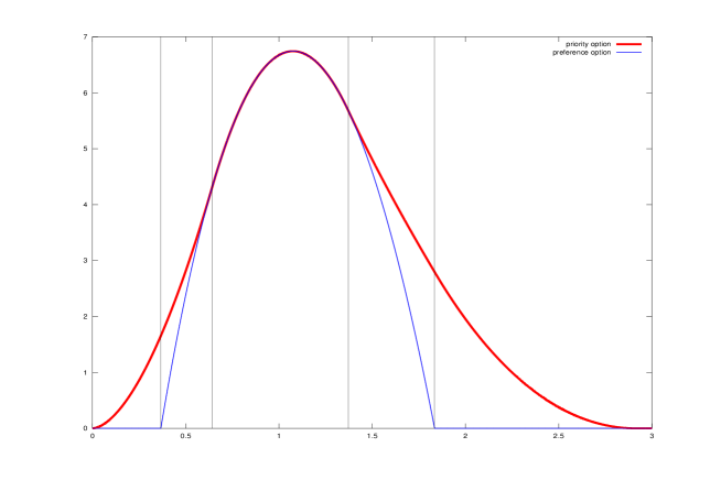
Following Grasselli et al. [7], we compare the advantage given by such an asymmetry to the usual Cournot game. In the latter, the positive difference between the Stackelberg leadership and the Cournot game provides a financial advantage which is called a priority option. By similarity, we call the marginal advantage of the weak Stackelberg advantage on the Cournot game a preference option.

Corollary 2.

Let us assume $q_{2}=q_{0}=0$. Let us denote $E_{1}^{(q_{1},q_{S})}(y)$ the expected payoff of agent one following from Theorem 3.3 when $(q_{1},q_{S})$ is given, for a level $y\in\mathbb{R}_{+}$. Then the preference option value is given by $\pi^{0}(y):=E_{1}^{(1,0)}(y)-E_{1}^{(0,1)}(y)$ for all $y\in\mathbb{R}_{+}$. Its value is equal to

$$\pi^{0}(y)=(L(y)-F(y))^{+}\quad\forall y\in\mathbb{R}_{+}\;.$$ (35)

Proof.

The proof is straightforward and follows from 26, where $E_{1}^{(0,1)}(y)=F(y)$ for $y\in[Y_{L},Y_{F}]$. Following Proposition 6, agent one shall invest at $\tau(Y_{L})$ if $y\leq Y_{L}$ at first. In this condition, his payoff is $L(Y_{L})=F(Y_{L})$, which provides 35. ∎

This option gives an advantage to its owner, agent one, without penalizing the other agent, who can always expect the payoff $F$. A comparison with the priority option is given in Figure 2.

Figure 2: Priority option value (red) and Preference option value (blue) in function of $y$. Vertical lines at $Y_{L}=0.37$, $Y_{1}=0.64$, $Y_{2}=1.37$ and $Y_{F}=1.83$. Option values are equal on $[Y_{1},Y_{2}]$. Same parameters as in Figure 1.

A very similar situation to the weak Stackelberg advantage can be observed if we take $q_{2}=0$ but $q_{S}>0$. The economic situation however loses a part of its meaning. It would convey the situation where agent two is accepted as investor only if he shares the market with agent one or become a follower. In this setting we can apply also the results of Section 3. We observe from definition 19 that in this case, $Y_{2}=Y_{F}$ and $Y_{1}$ verifies $F(Y_{1})=q_{1}L(Y_{1})+(1-q_{1})S(Y_{1})$. The consequence is straightforward: the interval $[Y_{1},Y_{2})$ expands to $[Y_{1},Y_{F})$. The fact that $Y_{1}>Y_{L}$ for $q_{1}<1$ has also a specific implication.

In that case, the equilibrium $(1,0)$ is more relevant than $(P_{1}(y),P_{2}(y))$ on $[Y_{L},Y_{1})$. Indeed, if agent one invests systematically on that interval then agent two has no chance of being the leader since $q_{2}=0$. Thus $p_{2}=0$ and the payoffs become

$$(E_{1}(y),E_{2}(y))=\left(L(y),F(y)\right)\text{ for }y\in[Y_{L},Y_{1})\;.$$ (36)

In opposition of the trembling-hand equilibrium, this pure strategy can be well figured by being called steady-hand Comparing 26 to 36, agent one shall use the pure strategy, whereas agent two is indifferent between the mixed and the pure strategy. Setting $q_{2}=0$ thus provides a preference option to agent one.

5 Aversion for confrontation

The introduction of the regulator rendering the market incomplete, utility indifference pricing can be invoked to evaluate payoffs. Although its action is purely random in the presented model, the regulator represents a third actor in the game. We study here the the impact of risk aversion on the coordination game only, which can be seen as an original dimension we denote aversion for confrontation.

5.1 Risk aversion in complete market

We keep the market model of Section 2. However, we now endow each agent with the same CARA utility function

$$U(x)=-\exp(-\gamma x)$$ (37)

where $\gamma>0$ is the risk-aversion of agents. The function $U$ is strictly concave and is chosen to avoid dependence on initial wealth. Recalling Remark 3, the market without regulator is complete and free of arbitrage, so that both agents still price the leader, the follower and sharing positions with the unique risk-neutral probability $\mathbb{Q}$. Thus, agents compare the utility of the different investment option market prices, denoted $l(y):=U(L(y))$, $f(y):=U(F(y))$ and $s(y):=U(S(y))$. The $s_{i}$, $i=1,2$ are defined the same way. When needed, variables will be indexed with $\gamma$ to make the dependence explicit. The definition of regulation is updated.

Definition 5.1.

Fix $t$ and $Y_{t}=y$. For $i=1,2$, if $j=3-i$ is the index of the opponent and $\tau_{j}$ his time of investment, then agent $i$ receives utility

$$r_{i}(t,y):=\left\{\begin{array}[]{ll}0&\text{if }\alpha=\alpha_{0}\\ l(y)\mathds{1}_{\{t\leq\tau_{j}\}}+f(y)\mathds{1}_{\{t>\tau_{j}\}}&\text{if }\alpha=\alpha_{i}\\ f(y)\mathds{1}_{\{t=\tau_{j}\}}&\text{if }\alpha=\alpha_{j}\\ l(y)\mathds{1}_{\{t<\tau_{j}\}}+s(y)\mathds{1}_{\{t=\tau_{j}\}}+f(y)\mathds{1}_{\{t>\tau_{j}\}}&\text{if }\alpha=\alpha_{S}\\ \end{array}\right.\;.$$ (38)

From Definition 5.1, it appears that by monotonicity of $U$, the game is strictly the same as in Section 2, apart from payoffs. Both agents defer for $y<Y_{L}$ and both act immediately for $y\geq Y_{F}$. The incomplete market setting is now handled with a utility maximization criterion. Each agent uses now a mixed strategy $p^{\gamma}_{i}$, in order to maximize an expected utility slightly different from 23 on $(Y_{L},Y_{F})$:

$$E^{\gamma}_{1}(y)=(a^{\gamma}_{1}+a^{\gamma}_{s}q_{1})l(y)+(a^{\gamma}_{2}+a^{\gamma}_{S}q_{2})f(y)+a^{\gamma}_{s}q_{S}s(y)$$ (39)

Results of Section 3 thus hold by changing $(L,F,S)$ for $(l,f,s)$. It follows that in that case

$$P_{i,\gamma}(y)=\frac{l(y)-f(y)}{q_{i}(l(y)-f(y))-q_{S}(l(y)-s(y))}\text{ with }i\in\{1,2\}$$ (40)

play the central role and that optimal strategic interaction of agents can be characterized by the value of $y$, or equivalently on the interval $[Y_{F},Y_{L}]$ by the values of $P_{1,\gamma}(y)$ and $P_{2,\gamma}(y)$. The question we address in this section is how risk-aversion influences the different strategic interactions.

5.2 Influence of $\gamma$ on strategies

First, aversion for confrontation is expressed through diminishing probability of intervention with $\gamma$.

Proposition 7.

Assume $q_{S}=1$, and $y\in(Y_{L},Y_{S})$. Denote $p_{\gamma}(y):=P_{1,\gamma}(y)=P_{2,\gamma}(y)$. Then $p_{\gamma}\leq p_{0}$ and furthermore,

$$\lim\limits_{\gamma\downarrow 0}p_{\gamma}=p_{0}\;\mbox{ and }\;\lim\limits_{\gamma\uparrow\infty}p_{\gamma}=0\;.$$ (41)

Proof.

According to 40 with $q_{S}=1$, $p_{\gamma}(y)\in(0,1)$ on $(Y_{L},Y_{S})$. From 40 we get

$$p_{\gamma}(y)=\frac{l(y)-f(y)}{l(y)-s(y)}=\frac{-e^{\gamma L(y)}+e^{\gamma F(y)}}{-e^{\gamma L(y)}+e^{\gamma S(y)}}=\frac{e^{\gamma(L-F(y))}-1}{e^{\gamma(L-S(y))}-1}\;.$$ (42)

Since $u(x):=-1-U(-x)=e^{\gamma x}-1$ is a positive strictly convex function on $\mathbb{R}_{+}$ with $u(0)=0$, we have that

$$p_{\gamma}(y)=\frac{u(L(y)-F(y))}{u(L(y)-S(y))}<\frac{L(y)-F(y)}{L(y)-S(y)}=:p_{0}(y)\;.$$ (43)

For $\gamma$ going to zero, we apply l’Hôpital’s rule to obtain that $\lim_{\gamma\downarrow 0}p_{\gamma}=p_{0}$. The other limit follows from expliciting the utility function:

$$\lim\limits_{\gamma\uparrow\infty}p_{\gamma}(y)=\lim\limits_{\gamma\uparrow\infty}e^{-\gamma(F(y)-S(y))}=0\;.$$ (44)

∎

Remark 9.

Notice that there is no uniform convergence since $p_{0}$ is continuous and $p_{0}(Y_{F})=1$. The above convergence holds for all $y\in[Y_{L},Y_{F})$. It is clear from 43 that $p_{\gamma}$ is monotonous in $\gamma$ on $\mathbb{R}_{+}^{*}$. Then according to 44, it is convex decreasing with $\gamma$.

For the general case $q_{S}<1$, the above result still holds, but on a reduced interval. Nevertheless, this interval depends on $\gamma$.

Proposition 8.

Assume $\min\{q_{1},q_{2},q_{S}\}>0$. Let $Y_{1,\gamma}\in[Y_{L},Y_{F}]$ be such that $P_{2,\gamma}(Y_{1,\gamma})=1$, and $Y_{2,\gamma}\in[Y_{L},Y_{F}]$ such that $P_{1,\gamma}(Y_{2,\gamma})=1$. Then for $i=1,2$, $Y_{i,\gamma}$ is increasing in $\gamma$ and

$$\lim\limits_{\gamma\uparrow\infty}Y_{i,\gamma}=Y_{F}\;.$$ (45)

Proof.

Consider $i\in\{1,2\}$. First notice that along Lemma 3, $Y_{i,\gamma}$ is uniquely defined on the designated interval. Following Remark 9, $P_{i,\gamma}$ is a concave non-decreasing functions of $p_{\gamma}$. It is then a decreasing function of $\gamma$. Since $P_{i,\gamma}(y)$ is decreasing with $\gamma$, $Y_{i,\gamma}$ is an increasing function of $\gamma$: the region $(Y_{L},Y_{1,\gamma})$ spreads on the right with $\gamma$. Adapting 19 to the present values, $Y_{i,\gamma}$ shall verify:

$$q_{i}(1-e^{\gamma(L(Y_{i,\gamma})-F(Y_{i,\gamma}))})+q_{S}(1-e^{\gamma(S(Y_{i,\gamma})-F(Y_{i,\gamma}))})=0$$

and when $\gamma$ goes to $\infty$, following 44, we need $L(Y_{i,\gamma})-F(Y_{i,\gamma})$ to go to 0, so that $Y_{i,\gamma}$ tends toward $Y_{F}$. ∎

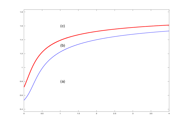
With risk aversion, the region (a) takes more importance and the competitive advantage of agent one decreases with $\gamma$. Figure 3 resumes the evolution.

Figure 3: Values of $Y_{1}$ (blue) and $Y_{2}$ (red) as a function of risk aversion $\gamma$. Y-axis limited to $[Y_{L},Y_{F}]=[0.37,1.83]$. Limit values of $(Y_{1},Y_{2})$ for $\gamma$ going to 0 corresponds to $(0.53,0.72)$ of Figure 1. Same parameters as previous figures.

The interval $(Y_{L},Y_{1,\gamma})$ describing the case (a) is the more relevant in terms of strategies, as the only one to involve mixed strategies. Propositions 7 and 8 imply the following result on this interval.

Corollary 3.

Assume $y\in[Y_{L},Y_{1,\gamma})$. Let $(a_{1}^{\gamma},a_{2}^{\gamma},a_{S}^{\gamma})$ be defined by 20, 21 and 22 where $(p_{1},p_{2})$ is replaced by $(P_{1,\gamma},P_{2,\gamma})$. Then

$$\lim\limits_{\gamma\uparrow\infty}a_{S}=0\;\mbox{ and }\;\lim\limits_{\gamma\uparrow\infty}\frac{a_{1}^{\gamma}}{a_{2}^{\gamma}}=1\;.$$ (46)

Proof.

Denote $p_{i}^{\gamma}:=P_{i,\gamma}$ and $p_{\gamma}:=(l(y)-f(y))/(l(y)-s(y))$ the equivalent of $p_{0}$ in the risk averse setting. From 22, $a_{S}^{\gamma}$ is a decreasing function of both $p_{1}^{\gamma}$ and $p_{2}^{\gamma}$, and the first limit is a straightforward consequence of 41.

Plugging 40 into $a_{i}^{\gamma}$, we obtain

$$a^{\gamma}_{i}=\frac{p_{i}^{\gamma}(1-p_{j}^{\gamma})}{p_{1}^{\gamma}+p_{2}^{\gamma}-p_{1}^{\gamma}p_{2}^{\gamma}},\quad i\neq j\in\{1,2\}^{2}\;,$$ (47)

and differentiating in $p_{\gamma}$, we obtain that $a^{\gamma}_{i}$ is increasing in $\gamma$. It also follows that

$$\frac{a^{\gamma}_{1}}{a^{\gamma}_{2}}=\frac{p^{\gamma}_{1}-p^{\gamma}_{1}p^{\gamma}_{2}}{p^{\gamma}_{2}-p^{\gamma}_{1}p^{\gamma}_{2}}=\frac{q_{S}-(1-q_{2})p_{\gamma}}{q_{S}-(1-q_{1})p_{\gamma}}\leq 1\;.$$ (48)

The second limit of 46 follows immediately from Proposition 7. ∎

Remark 10.

We can easily assert as in Proposition 7 that $a_{S}^{\gamma}<a_{S}$ for any $\gamma>0$, where $a_{S}$ is the probability of simultaneous action in the game for risk-neutral agents. Equivalently,

$$\frac{a_{1}}{a_{2}}=\frac{F(y)-S_{1}(y)}{F(y)-S_{2}(y)}<\frac{a_{1}^{\gamma}}{a_{2}^{\gamma}},\quad\forall\gamma>0\;.$$ (49)

The above results can be interpreted as follows. The parameter $\gamma$ is an aversion for the uncertainty following from the coordination game and the regulatory intervention. As expected, the higher this parameter, the lower the probability to act $P_{i,\gamma}$ in the game. However the game being infinitely repeated until action of at least one agent, for values of $P_{i,\gamma}$ lower than one, the game is extended to a bigger interval $[Y_{L},Y_{1,\gamma})$ with $\gamma$. Then, it naturally reduces simultaneity of investment, but tends also to an even chance of becoming a leader for both agents. There is thus a consequence to a high risk-aversion $\gamma$: agents synchronize to avoid playing the game and the regulator decision. In some sense, the behavior in a Stackelberg competition is the limit with risk-aversion of the behavior of competitors in a Cournot game.

How does $\gamma$ impact the outcome of the game? As above since we are in complete market, the risk aversion makes no relevant modification to the cases where the coordination game is not played. On the interval $(Y_{L},Y_{1,\gamma})$ then, we need to compare the expected values of options $L,F$ and $S$ to homogeneously quantities.

Proposition 9.

For $y\in[Y_{L},Y_{1,\gamma})$, let $E_{1}^{\gamma}(y)$ be the expected utility of agent one in the coordination game when strategies $(P_{1,\gamma}(y),P_{2,\gamma}(y))$ are played. Then the indifference value of the game for agent one is given by

$$e_{1,\gamma}(y):=U^{-1}(E_{1}^{\gamma}(y))=-\frac{1}{\gamma}\log\left(-a^{\gamma}_{1}l(y)-a^{\gamma}_{2}f(y)-a^{\gamma}_{S}s_{i}(y)\right)\;.$$ (50)

We define $e_{2,\gamma}$ similarly. Assume now $q_{S}>0$. For $y\in[Y_{L},Y_{1,\gamma})$, we have for $i=1,2$ that

$$e_{i,\gamma}(y)=E_{i}(y)=F(y)\quad\forall\gamma>0\;,$$ (51)

with $E_{i}(y)$ defined in 26.

Proof.

Using 47, we can proceed as in the end of Section 3 to retrieve

$$a_{1,\gamma}l(y)+a_{2,\gamma}f(y)+a_{S,\gamma}s_{i}(y)=f(y),\quad i=1,2\;,$$ (52)

and 51 follows from the definition of $e_{i,\gamma}$. ∎

Risk-aversion in complete market has thus the interesting property to keep true the rent equalization principle of Fudenberg and Tirole [6]: agents adapt their strategies to be indifferent between playing the game or obtaining the follower’s position.

6 Criticism and extensions

If real option games model are to be applied, the role of a regulator shall be introduced in order to suit realistic situations of competition. Indeed regulators often intervene for important projects in energy, territorial acquisition and highly sensitive products such as drugs. Despite its simplicity and its idealization, the present model has still something to say. One can see it as an archetype model, unifying mathematically the Stackelberg and the Cournot competition frameworks and leading to simple formulas. The model we proposed is a first attempt, and could be improved on several grounds. Three main objections can be raised.

As observed in Remark 4 of Section 3, the extention of strategies in 2.5 in the fashion of Fudenberg and Tirole [6] has unrealistic and strongly constrained implications due to continuous time and perfect information. This is emphasized here in the interpretation that the regulator can only intervene when agents simultaneously invest. A prioritize objective would be to propose a new setting for the standard game conveying a dynamical dimension to strategies.

A realistic but involved complication is the influence of explicit parameters on the law $\mathbb{P}^{+}$, parameters on which agents have some control. The value of being preferred, introduced as a financial option in subsection 4.3, would then provide a price to a competitive advantage and to side efforts to satisfy non-financial criteria. Eventually, a game with the regulator as a third player appears as a natural track of inquiry.

Finally, the introduction of risk-aversion should not be restrained to the coordination game. This issue is already tackled in Bensoussan et al. [3], and Grasselli et al. [7] for the incomplete market setting. But as a fundamentally different source of risk, the coordination game and the regulator’s decision shall be evaluated with a different risk-aversion parameter, as we proposed in Section 5. An analysis of asymmetrical risk aversion as in Appendix C of Grasselli et al. [7] shall naturally be undertaken.

References

- [1] A.F. Azevedo and D.A. Paxson, Real options game models: A review, Real Options 2010, 2010.
- [2] F. Black and M. Scholes, The pricing of options and corporate liabilities, The journal of political economy (1973), 637–654.
- [3] A. Bensoussan, J.D. Diltz and S. Hoe, Real options games in complete and incomplete markets with several decision makers, SIAM Journal on Financial Mathematics, 1(2010), 666–728.
- [4] D. Becherer, Rational hedging and valuation of integrated risks under constant absolute risk aversion, Insurance: Mathematics and economics, 33 (2003), 1–28.
- [5] B. Chevalier-Roignant, C.M Flath, A. Huchzermeier and L. Trigeorgis, Strategic investment under uncertainty: a synthesis, European Journal of Operational Research, 215 (2011), 639–650.
- [6] D. Fudenberg and J. Tirole, Preemption and rent equalization in the adoption of new technology. The Review of Economic Studies, 52 (1985), 383–401.
- [7] M. Grasselli, V. Leclere and M. Ludkovski, Priority Option: The Value of Being a Leader, International Journal of Theoretical and Applied Finance, 16.01, 2013.
- [8] S.R. Grenadier, The strategic exercise of options: Development cascades and overbuilding in real estate markets, The Journal of Finance, 51 (1996), 1653–1679.
- [9] S.R. Grenadier, Option exercise games: the intersection of real options and game theory, Journal of Applied Corporate Finance, 13 (2000), 99–107.
- [10] C-f Huang and L. Lode, Entry and exit: Subgame perfect equilibria in continuous-time stopping games, working paper, 1991.
- [11] D. Paxson and H. Pinto, Rivalry under price and quantity uncertainty, Review of Financial Economics, 14 (2005), 209–224.
- [12] F. Smets, F., “Essays on Foreign Direct Investment”, Ph.D. Thesis, Yale University, 1993.
- [13] A. Tsekrekos, The effect of first-mover’s advantages on the strategic exercise of real option, in “Real R&D Options” (eds. D. Paxson), Butterworth-Heinemann (2003), 185–207.
- [14] J.J. Thijssen, Preemption in a real option game with a first mover advantage and player-specific uncertainty, Journal of Economic Theory, 145 (2010), 2448–2462.
- [15] J.J. Thijssen, K.J. Huisman and P.M. Kort, Symmetric equilibrium strategies in game theoretic real option models, CentER DP 81, 2002.
- [16] H. Weeds, Strategic delay in a real options model of R&D competition, The Review of Economic Studies, 69(2002), 729–747.