On quadrilateral orbits in complex algebraic planar billiards

Abstract

The famous conjecture of V.Ya.Ivrii (1978) says that in every billiard with infinitely-smooth boundary in a Euclidean space the set of periodic orbits has measure zero. In the present paper we study the complex algebraic version of Ivrii’s conjecture for quadrilateral orbits in two dimensions, with reflections from complex algebraic curves. We present the complete classification of 4-reflective algebraic counterexamples: billiards formed by four complex algebraic curves in the projective plane that have open set of quadrilateral orbits. As a corollary, we provide classification of the so-called real algebraic pseudo-billiards with open set of quadrilateral orbits: billiards formed by four real algebraic curves; the reflections allow to change the side with respect to the reflecting tangent line.

To my dear teacher Yu.S.Ilyashenko on the occasion of his 70-th birthday

1 Introduction

1.1 Main result: the classification of 4-reflective complex planar algebraic billiards

The famous V.Ya.Ivrii’s conjecture [10] says that in every billiard with infinitely-smooth boundary in a Euclidean space of any dimension the set of periodic orbits has measure zero. As it was shown by V.Ya.Ivrii [10], his conjecture implies the famous H.Weyl’s conjecture on the two-term asymptotics of the spectrum of Laplacian [23]. A brief historical survey of both conjectures with references is presented in [6, 7].

For the proof of Ivrii’s conjecture it suffices to show that for every $k\in\mathbb{N}$ the set ot $k$-periodic orbits has measure zero. For $k=3$ this was proved in [2, 16, 18, 24] for dimension two and in [22] for any dimension. For $k=4$ in dimension two this was proved in [6, 7].

Remark 1.1

Ivrii’s conjecture is open already for piecewise-analytic billiards, and we believe that this is its principal case. In the latter case Ivrii’s conjecture is equivalent to the statement saying that for every $k\in\mathbb{N}$ the set of $k$-periodic orbits has empty interior.

In the present paper we study a complexified version of Ivrii’s conjecture in complex dimension two. More precisely, we consider the complex plane $\mathbb{C}^{2}$ with the complexified Euclidean metric, which is the standard complex-bilinear quadratic form $dz_{1}^{2}+dz_{2}^{2}$. This defines notion of symmetry with respect to a complex line, reflections with respect to complex lines and more generally, reflections of complex lines with respect to complex analytic (algebraic) curves. The symmetry is defined by the same formula, as in the real case. More details concerning the complex reflection law are given in Subsection 2.1. One could have replaced the initial real Euclidean metric by a pseudo-Euclidean one: the geometry of the latter is somewhat similar to that of our complex Euclidean metric. Billiards in pseudo-Euclidean spaces were studied, e.g., in [4, 11]. Proofs of the classical Poncelet theorem and its generalizations by using complex methods can be found in [8, 17].

To formulate the complexified Ivrii’s conjecture, let us introduce the following definitions.

Definition 1.2

A complex projective line $l\subset\mathbb{CP}^{2}\supset\mathbb{C}^{2}$ is isotropic, if either it coincides with the infinity line, or the complexified Euclidean quadratic form vanishes on $l$. Or equivalently, a line is isotropic, if it passes through some of two points with homogeneous coordinates $(1:\pm i:0)$: the so-called isotropic points at infinity (also known as cyclic (or circular) points).

Definition 1.3

A complex analytic (algebraic) planar billiard is a finite collection of complex irreducible analytic (algebraic) curves $a_{1},\dots,a_{k}$ that are not isotropic lines; we set $a_{k+1}=a_{1}$, $a_{0}=a_{k}$. A $k$-periodic billiard orbit is a collection of points $A_{j}\in a_{j}$, $A_{k+1}=A_{1}$, $A_{0}=A_{k}$, such that for every $j=1,\dots,k$ one has $A_{j+1}\neq A_{j}$, the tangent line $T_{A_{j}}a_{j}$ is not isotropic and the complex lines $A_{j-1}A_{j}$ and $A_{j}A_{j+1}$ are symmetric with respect to the line $T_{A_{j}}a_{j}$ and are distinct from it. (Properly saying, we have to take vertices $A_{j}$ together with prescribed branches of curves $a_{j}$ at $A_{j}$: this specifies the line $T_{A_{j}}a_{j}$ in unique way, if $A_{j}$ is a self-intersection point of the curve $a_{j}$.)

Definition 1.4

A complex analytic (algebraic) billiard $a_{1},\dots,a_{k}$ is $k$-reflective, if it has an open set of $k$-periodic orbits. In more detail, this means that there exists an open set of pairs $(A_{1},A_{2})\in a_{1}\times a_{2}$ extendable to $k$-periodic orbits $A_{1}\dots A_{k}$. (Then the latter property automatically holds for every other pair of neighbor mirrors $a_{j}$, $a_{j+1}$.)

Problem (Complexified version of Ivrii’s conjecture). Classify all the $k$-reflective complex analytic (algebraic) billiards.

Contrarily to the real case, where there are no piecewise $C^{4}$-smooth 4-reflective planar billiards [6, 7], there exist 4-reflective complex algebraic planar billiards. In the present paper we classify them (Theorem 1.11 stated at the end of the subsection). Basic families of 4-reflective algebraic planar billiards are given below. Theorem 1.11 shows that their straightforward analytic extensions cover all the 4-reflective algebraic planar billiards.

Remark 1.5

An $l$-reflective analytic (algebraic) billiard generates $ml$-reflective analytic (algebraic) billiards for all $m\in\mathbb{N}$. Therefore, $k$-reflective billiards exist for all $k\equiv 0(mod4)$.

Now let us pass to the construction of 4-reflective complex billiards. The construction comes from the real domain, and we use the following relation between real and complex reflection laws in the real domain.

Remark 1.6

In a real billiard the reflection of a ray from the boundary is uniquely defined: the reflection is made at the first point where the ray meets the boundary. In the complex case, the reflection of lines with respect to a complex analytic curve is a multivalued mapping (correspondence) of the space of lines in $\mathbb{CP}^{2}$: we do not have a canonical choice of intersection point of a line with the curve. Moreover, the notion of interior domain does not exist in the complex case, since the mirrors have real codimension two. Furthermore, the real reflection law also specifies the side of reflection. Namely, a triple of points $A,B,C\in\mathbb{R}^{2}$, $A\neq B$, $B\neq C$, and a line $L\subset\mathbb{R}^{2}$ through $B$ satisfy the real reflection law, if the lines $AB$ and $BC$ are symmetric with respect to $L$, and also the points $A$ and $C$ lie in the same half-plane with respect to the line $L$. The complex reflection law says only that the complex lines $AB$ and $BC$ are symmetric with respect to $L$ and does not specify the positions of the points $A$ and $C$ on these lines: they may be arbitrary. A triple of real points $A,B,C\in\mathbb{R}^{2}$, $A\neq B$, $B\neq C$ and a line $L\subset\mathbb{R}^{2}$ through $B$ satisfy the complex reflection law, if and only if

- either they satisfy the usual real reflection law (and then $A$ and $C$ lie on the same side from the line $L$),

- or the line $L$ is the bissectrix of the angle $ABC$ (and then $A$ and $C$ lie on different sides from the line $L$).

In the latter case we say that the triple $A$, $B$, $C$ and the line $L$ satisfy the skew reflection law.

Example 1.7

Consider the following complex billiard with four mirrors $a$, $b$, $c$, $d$: $a=c$ is a non-isotropic complex line; $b$ is an arbitrary analytic (algebraic) curve distinct from $a$; $d$ is symmetric to $b$ with respect to the line $a$. This complex billiard obviously has an open set of 4-periodic orbits $ABCD$, these orbits are symmetric with respect to the line $a$, see Fig.1.

Figure 1: 4-reflective billiards symmetric with respect to a line mirror: real pictures

Example 1.8

Consider a complex billiard formed by four distinct lines $a$, $b$, $c$, $d$ passing through the same point $O\in\mathbb{CP}^{2}$ such that the line pairs $(a,b)$ and $(d,c)$ (or equivalently, $(a,d)$ and $(b,c)$) are unimodularly isometric. That is, there exists a complex Euclidean isometry with unit Jacobian that transforms one pair into the other: a complex rotation around the intersection point $O$, see Fig.2. This billiard is 4-reflective, or equivalently, the composition of symmetries $\sigma_{g}$, $g=a,b,c,d$, with respect to the lines $a$, $b$, $c$ and $d$ that act on the dual projective plane is identity: $\sigma_{a}\circ\sigma_{b}\circ\sigma_{c}\circ\sigma_{d}=Id$ on $\mathbb{CP}^{2*}$. Indeed, the latter identity is equivalent to the same identity on the projective plane, i.e., $\sigma_{a}\circ\sigma_{b}=\sigma_{d}\circ\sigma_{c}$ on $\mathbb{CP}^{2}$. The latter holds if there exists a complex rotation around $O$ sending the pair $(a,b)$ to $(d,c)$. This follows from the fact that the composition of symmetries with respect to two lines through a point $O$ is a complex rotation around $O$ and the commutativity of the group of complex rotations around $O$. Let us prove the converse: assuming the same identity we show that $(d,c)$ is obtained from $(a,b)$ by complex rotation around $O$. Let $c^{\prime}$ denote the image of the line $b$ under the complex rotation sending $a$ to $d$. One has $\sigma_{a}\circ\sigma_{b}=\sigma_{d}\circ\sigma_{c^{\prime}}=\sigma_{d}\circ\sigma_{c}$, by the previous statement and assumption. Therefore, $\sigma_{c^{\prime}}=\sigma_{c}$, hence $c^{\prime}=c$.

Figure 2: 4-reflective billiards on two unimodularly isometric line pairs: real pictures

Example 1.9

Consider the complex billiard with four mirrors $a$, $b$, $c$, $d$: $a=c$ and $b=d$ are complexifications of two distinct concentric circles on the real plane. Say, $a=c$ is the smaller circle. We say that we reflect from the bigger circle $b=d$ in the usual way, ”from interior to interior”, and we reflect from the smaller circle in the skew way: ”from interior to exterior” and vice versa. Take arbitrary points $A\in a$ and $B\in b$ such that the segment $AB$ lies outside the disk bounded by $a$. Let $R$ denote the ray symmetric to the ray $BA$ with respect to the diameter through $B$. Let $C$ denote its second intersection point with the smaller circle mirror $a=c$. (We say that the ray $R$ passes through the first intersection point ”without noticing the mirror $a$”.) Consider the symmetry with respect to the diameter orthogonal to the line $AC$. Let $D\in b=d$ denote the symmetric image of the point $B$, see Fig.3. Thus, we have constructed a self-intersected quadrilateral $ABCD$ depending analytically on two parameters: $A\in a$ and $B\in b$.

Figure 3: A 4-reflective billiard on concentric circles

Claim. The above quadrilateral $ABCD$ is a 4-periodic orbit of the complex billiard $a$, $b$, $c$, $d$, and the billiard is 4-reflective.

Proof.

The reflection law is obviously satisfied at the vertices $B,D\in b=d$. It suffices to check the skew reflection law at the vertices $A,C\in a$. By symmetry, it suffices to show that the tangent line $T_{A}a$ is the bissectrix of the angle $BAD$. The union of lines $AD$ and $BC$ intersects the circle $a$ at four points with equal intersection angles, since these lines are symmetric with respect to a diameter. Similarly, the lines $AB$ and $BC$ intersect the circle $a$ at equal angles: they are symmetric with respect to the diameter through $B$. The two latter statements together imply that the tangent line $T_{A}a$ is the bissectrix of the angle $BAD$. Thus, we have a two-parametric quadrilateral orbit family $ABCD$ that extends analytically to complex domain. Hence, the billiard is 4-reflective. This proves the claim. ∎

Consider a generalization of the above example: a complex billiard $a$, $b$, $c$, $d$ similar to the above one, but now $a=c$ and $b=d$ are complexifications of distinct confocal ellipses, say, $a=c$ is the smaller one.

Theorem 1.10

(M.Urquhart, see [20, p.59, corollary 4.6]). The above two confocal ellipse billiard $a$, $b$, $a$, $b$, see Fig.4, is 4-reflective.

Figure 4: A 4-reflective billiard on confocal ellipses

The main result of the paper is the following theorem.

Theorem 1.11

A complex planar algebraic billiard $a$, $b$, $c$, $d$ is 4-reflective, if and only if it has one of the following types:

Case 1): some mirror, say $a$ is a line, $a=c$, and the curves $b,d\neq a$ are symmetric with respect to the line $a$, cf. Example 1.7, Fig.1.

Case 2): $a$, $b$, $c$, $d$ are distinct lines through the same point $O\in\mathbb{CP}^{2}$; the line pair $(a,b)$ is sent to $(d,c)$ by complex rotation around $O$, cf. Example 1.8, Fig.2.

Case 3): $a=c$, $b=d$ and they are distinct confocal conics, cf. Theorems 1.10 and 2.25, Fig.3, 4.

Remark 1.12

The notion of confocality of complex conics is the immediate analytic extension to complex domain of confocality of real conics. See more precise Definition 2.24 in Subsection 2.4.

Remark 1.13

There is an analogue of Ivrii’s conjecture in the invisibility theory: Plakhov’s invisibility conjecture [13, conjecture 8.2, p.274]. Its complexification coincides with the above complexified Ivrii’s conjecture [5]. For more results on invisibility see [1, 13, 14, 15]. Another analogue of the 4-reflective planar Ivrii’s conjecture is Tabachnikov’s commuting billiard problem [19, p.58, the last paragraph]; their complexifications coincide. Thus, results about the complexified Ivrii’s conjecture have applications not only to the original Ivrii’s conjecture, but also to Plakhov’s invisibility conjecture and Tabachnikov’s commuting billiard problem.

1.2 Plan of the proof of Theorem 1.11 and structure of the paper

Theorem 1.11 is proved in Sections 2–4. In Section 6 we present its application (Theorem 6.3), which gives the classification of so-called 4-reflective real algebraic pseudo-billiards: billiards that have open set of 4-periodic orbits with skew reflection law at some vertices and usual at the other ones.

The definition of confocal complex conics and the proof of 4-reflectivity of a billiard $a$, $b$, $a$, $b$ on distinct confocal conics $a$ and $b$ (Theorem 2.25) are given in Subsection 2.4. The 4-reflectivity of billiards of types 1) and 2) in Theorem 1.11 was already explained in Examples 1.7 and 1.8.

The main part of Theorem 1.11 saying that each 4-reflective planar algebraic billiard $a$, $b$, $c$, $d$ is of one of the types 1)–3) is proved in Subsection 2.3 and Sections 3, 4. The main idea of the proof is similar to that from [6, 7]: to study the “degenerate” limits of open set of quadrilateral orbits, i.e., quadrilaterals having either an edge tangent to a mirror at an adjacent vertex, or a pair of coinciding neighbor vertices, or a vertex that is an isotropic tangency point of the corresponding mirror. We deal with the compact Riemann surfaces $\hat{a}$, $\hat{b}$, $\hat{c}$, $\hat{d}$, the so-called normalizations of the curves $a$, $b$, $c$, $d$ respectively that parametrize them bijectively except for self-intersections. We study the closure in $\hat{a}\times\hat{b}\times\hat{c}\times\hat{d}$ of the open set of 4-periodic orbits in the usual topology. This is a purely two-dimensional algebraic set, which we will call the 4-reflective set and denote $U$, that contains a Zariski open and dense subset $U_{0}\subset U$ of 4-periodic billiard orbits (Proposition 2.14). The above-mentioned degenerate quadrilaterals form the complement $U\setminus U_{0}$. The proof of Theorem 1.11 consists of the following steps.

Step 1. Description of a large class of degenerate quadrilaterals $ABCD\in U\setminus U_{0}$ (Subsections 2.1 and 2.2).

1A) Case, when some vertex, say $B$ is an isotropic tangency point of the corresponding mirror $b$. We prove the isotropic reflection law: if $B\neq A,C$, then at least one of the lines $AB$, $BC$ coincides with the isotropic tangent line $T_{B}b$. (Propositions 2.7 and 2.14 in Subsection 2.1)

1B) Case, when some edge is tangent to the mirror through an adjacent vertex, say, $AB=T_{B}b$. We show that this cannot be the only degeneracy (Proposition 2.16). We show that the case, when $AB=T_{B}b$, $b=c$ and $B=C$ is also impossible without other degeneracies (Proposition 2.18). We then deduce (Corollary 2.19) that no 4-reflective algebraic planar billiard can have a pair of coinciding neighbor mirrors, say $b=c$. This is done by contradiction: assuming the contrary, we deform a quadrilateral orbit $ABCD$ to a limit quadrilateral with $B=C$ forbidden by Proposition 2.18.

1C) Case, when $AB=T_{B}b$ and it is not an isotropic line, and there are no degeneracies at the neighbor vertices $A$ and $C$. We show that either $AD=T_{D}d$, $A=C$ and $a=c$, or $D$ is a cusp with non-isotropic tangent line (Corollary 2.20 in Subsection 2.2). This follows from Proposition 2.16 and the fact (proved in the same subsection) that there exists no one-parameter family of quadrilaterals $ABCD\in U$ with $C,D\in AB=T_{B}b=T_{D}d$. Corollary 2.20 implies Corollary 2.21 saying that if the mirror $b$ is not a line and $d$ has no cusps with non-isotropic tangent lines, then $a=c$.

Step 2. Proof of Theorem 1.11 in the case, when some of the mirrors, say $a$ is a line (Proposition 2.22 in Subsection 2.3). In the subcase, when some its neighbor mirror, say $b$ is not a line, this is done by considering a one-parametric family $\mathcal{T}$ of degenerate quadrilaterals $ABCD\in U$ with $AB=T_{B}b$. The above-mentioned Corollary 2.20 together with the reflection law at $A$ imply that for every $ABCD\in\mathcal{T}$ one has $AD=T_{D}d$, the vertices $B$, $D$ are symmetric with respect to the line $a$ (an elementary projective duality argument) and $a=c$. Thus, the billiard is of type 1) in Theorem 1.11. In the subcase, when $a$, $b$ and $d$ are lines, the above arguments applied to $b$ instead of $a$ imply that $c$ is also a line. The composition of symmetries with respect to the lines $a$, $b$, $c$ and $d$ acting on the dual projective plane is identity, by 4-reflectivity. Hence, the billiard is of type 2), if the lines are distinct, and of type 1) otherwise.

The rest of the proof concerns the case, when no mirror is a line.

Step 3. Birationality of neighbor edge correspondence and rationality of mirrors (Subsection 3.1). The image of the projection $U\to\hat{b}\times\hat{a}\times\hat{d}$ is a two-dimensional projective algebraic variety. It defines an algebraic correspondence $\psi_{a}:\hat{b}\times\hat{a}\to\hat{a}\times\hat{d}:$ $(B,A)\mapsto(A,D)$ for every $ABCD\in U$. First we prove (Lemma 3.1) that $\psi_{a}$ is birational, by contradiction. The contrary assumption implies that some of the transformations $\psi_{a}^{\pm 1}$, say $\psi_{a}$ has two holomorphic branches on some open subset $V\subset\hat{b}\times\hat{a}$: every $(A,B)\in V$ completes to two distinct 4-periodic orbits $ABCD,ABC^{\prime}D^{\prime}\in U_{0}$. It follows that the quadrilaterals $CDD^{\prime}C^{\prime}$ form a two-parameter family of 4-periodic orbits of the billiard $c$, $d$, $d$, $c$ with coinciding neighbor mirrors, and the latter billiard is 4-reflective, – a contradiction to Corollary 2.19 (Step 1B)). Next we prove that the mirrors are rational curves (Corollary 3.2). The proof is based on the observation that for every isotropic tangency point $A\in\hat{a}$ the transformation $\psi_{a}$ contracts the curve $\hat{b}\times A$ to a point $(A,D)$ with $\pi_{d}(D)\in T_{A}a\cap d$ (follows from the isotropic reflection law, see Proposition 2.14, Step 1A)). Applying the classical Indeterminacy Resolution Theorem ([9], p.545 of the Russian edition) to the inverse $\psi_{a}^{-1}$ yields that the curve $b$ is rational. At the end of Subsection 3.1 we deduce Corollary 3.4, which deals with one-parametric family $\Gamma$ of quadrilaterals $ABCD\in U\setminus U_{0}$ with $D$ being a fixed cusp with isotropic tangent line. It shows that $B\equiv const$ on $\Gamma$ and $B$ is a cusp of the same degree, as $D$.

Step 4. We show that all the mirrors have common isotropic tangent lines and each mirror has the so-called property (I): all the isotropic tangencies are of maximal order, i.e., the intersection of each mirror, say $a$ with its isotropic tangent line corresponds to a single point of its normalization $\hat{a}$ (Lemma 3.5 in Subsection 3.2). Namely, given an isotropic tangency point $A\in\hat{a}$ of the curve $a$, we have to show that the curve $d$ intersects the line $L=T_{A}a$ at a single point. This is equivalent to the statement saying that for every $D\in\hat{d}$ with $\pi_{d}(D)\in d\cap L$ the mapping $\psi_{a}$ contracts the curve $\hat{b}\times A$ to the point $(A,D)$. Or in other words, the projection to $\hat{b}\times\hat{a}\times\hat{d}$ of the graph of the birational correspondence $\psi_{a}$ contains the curve $\hat{b}\times A\times D$. The proof of this statement is split into the following substeps.

4A) Proof of the local version of the latter inclusion (Lemma 2.45 in Subsection 2.6), which deals with two distinct irreducible germs of analytic curves $(a,A),(b,B)\subset\mathbb{CP}^{2}$ such that the line $L=T_{A}a$ is isotropic and $B\in L$. Its statement concerns the germ of two-dimensional analytic subset $\Pi_{ab}$ in $b\times a\times\mathbb{CP}^{2*}$ at the point $(B,A,L)$ defined as follows: we say that $(B^{\prime},A^{\prime},L^{\prime})\in\Pi_{ab}$, if $A^{\prime}\in L^{\prime}$ and either $(A^{\prime},L^{\prime})=(A,L)$, or $(B^{\prime},A^{\prime})=(B,A)$, or the lines $A^{\prime}B^{\prime}$ and $L^{\prime}$ are symmetric with respect to the tangent line $T_{A^{\prime}}a$. By definition, the germ $\Pi_{ab}$ contains the germ of the curve $b\times A\times L$. Lemma 2.45 states that under a mild additional condition the germ $\Pi_{ab}$ is irreducible. The most technical part of the paper is the proof of Lemma 2.45 in the case, when the germs $a$ and $b$ are tangent to each other. The additional condition from the lemma is imposed only in the case of germs tangent to each other at a finite point and is formulated in terms of their Puiseaux exponents: the germs are represented as graphs of multivalued functions in appropriate coordinates, and we take the lower powers in their Puiseaux expansions. The above additional condition is satisfied automatically, if either the germ $a$ is smooth, or its Puiseaux exponent is no less than that of the germ $b$. The proof of Lemma 2.45 for tangent germs is based on Proposition 2.50 from Subsection 2.6, which deals with the family of tangent lines to $b$. It relates the asymptotics of the tangency point with that of the intersection points of the tangent line with the curve $a$.

4B) We cyclically rename the mirrors so that the mirror $a$ has a germ tangent to $L$ that satisfies the condition of Lemma 2.45 for every branch of the curve $b$ at its intersection point with $L$. This will be true, e.g., if we name $a$ the curve having a tangent germ to $L$ that is either smooth, or at an infinite point, or with the maximal possible Puiseaux exponent. We show that each one of the curves $d$ and $b$ intersects the line $L$ at a unique point. This follows from the irreducibility of the germ $\Pi_{ab}$ (Lemma 2.45), by elementary topological argument given by Proposition 2.47.

4C) We show that each one of the curves $\hat{a}$ and $\hat{c}$ intersects the line $L$ at a unique point. In the case, when the intersection point $D=d\cap L$ is either infinite, or smooth, this follows by applying Step 4B) to the curve $d$ instead of $a$. Otherwise, if $D$ is a finite cusp, we show that the curves $a$ and $c$ are conics with focus $D$, by using Corollary 3.4 (Step 3) and Proposition 2.32 (Subsection 2.4). Finally, we show that $a=c$, by using Corollary 2.21 (Step 1C)) and proving that the curve $d$ has no cusps with non-isotropic tangent lines. The latter statement is proved by applying Riemann-Hurwitz Formula to the projection $d\to\mathbb{CP}^{1}$ from appropriate point: the intersection point of two isotropic tangent lines to $a$.

Step 5. We show that the opposite mirrors coincide: $a=c$, $b=d$. This follows immediately from Corollary 2.21 and absence of cusps with non-isotropic tangent lines in rational curves with property (I). The latter follows from the description of rational curves with property (I) having cusps (Corollary 2.44 in Subsection 2.5).

Step 6. We prove that the mirrors are conics (Theorem 4.1 in Subsection 4.1). To do this, first we show that they have no cusps (Lemma 4.2). Assuming the contrary, we show that a mirror with cusps should have two distinct cusps of equal degrees (basically follows from Corollary 3.4, Step 3). This would contradict the above-mentioned Corollary 2.44, which implies that there are at most two cusps and their degrees are distinct. The rest of the proof of Theorem 4.1 is based on the fact that for every $A\in a$ with non-isotropic tangent line $T_{A}a$ the collection of the tangent lines to $b$ through $A$ is symmetric with respect to $T_{A}a$ (Corollary 3.6, which follows immediately from Corollary 2.20, Step 2). We apply Corollary 3.6 as $A$ tends to an isotropic tangency point, and deduce from symmetry that the isotropic tangency should be quadratic. In the case, when $a$ and $b$ are tangent to some isotropic line at distinct finite points, this is done by elementary local analysis. In the case, when $a$ and $b$ are isotropically tangent to each other, the proof is slightly more technical and uses Proposition 2.50, see Step 4A).

Step 7. We prove that the conics $a=c$ and $b=d$ are confocal (Subsection 4.2), by using confocality criterion given by Lemma 2.35 in Subsection 2.4. If one of them is transverse to the infinity line, then their confocality immediately follows from the lemma and the coincidence of their isotropic tangent lines. In the case, when both $a$ and $b$ are tangent to the infinity line, the proof is slightly more technical and is done by using the above-mentioned Corollary 3.6 and Proposition 2.50.

2 Preliminaries

2.1 Complex reflection law and nearly isotropic reflections.

We fix an Euclidean metric on $\mathbb{R}^{2}$ and consider its complexification: the complex-bilinear quadratic form $dz_{1}^{2}+dz_{2}^{2}$ on the complex affine plane $\mathbb{C}^{2}\subset\mathbb{CP}^{2}$. We denote the infinity line in $\mathbb{CP}^{2}$ by $\overline{\mathbb{C}}_{\infty}=\mathbb{CP}^{2}\setminus\mathbb{C}^{2}$.

Definition 2.1

The symmetry $\mathbb{C}^{2}\to\mathbb{C}^{2}$ with respect to a non-isotropic complex line $L\subset\mathbb{CP}^{2}$ is the unique non-trivial complex-isometric involution fixing the points of the line $L$. For every $x\in L$ it acts on the space $\mathcal{M}_{x}=\mathbb{CP}^{1}$ of lines through $x$, and this action is called symmetry at $x$. If $L$ is an isotropic line through a finite point $x$, then a pair of lines through $x$ is called symmetric with respect to $L$, if it is a limit of pairs of lines $(l_{1}^{n},l_{2}^{n})$ through points $x_{n}\to x$ such that $l_{1}^{n}$ and $l_{2}^{n}$ are symmetric with respect to non-isotropic lines $L_{n}$ through $x_{n}$ converging to $L$.

Remark 2.2

If $L$ is a non-isotropic line, then its symmetry is a projective transformation. Its restriction to the infinity line is a conformal involution. The latter is conjugated to the above action on $\mathcal{M}_{x}$ via the projective isomorphism $\mathcal{M}_{x}\simeq\overline{\mathbb{C}}_{\infty}$ sending a line to its intersection point with $\overline{\mathbb{C}}_{\infty}$.

Lemma 2.3

Let $L$ be an isotropic line through a finite point $x$. Two lines through $x$ are symmetric with respect to $L$, if and only if some of them coincides with $L$.

Let us introduce an affine coordinate $z$ on $\overline{\mathbb{C}}_{\infty}$ in which the isotropic points $I_{1}=(1:i:0)$, $I_{2}=(1:-i:0)$ at infinity be respectively $0$ and $\infty$. As it is shown below, Lemma 2.3 is implied by the following proposition

Proposition 2.4

The symmetry with respect to a finite non-isotropic line through a point $\varepsilon\in\overline{\mathbb{C}}_{\infty}\setminus\{0,\infty\}$ acts on $\overline{\mathbb{C}}_{\infty}$ by the formula $z\mapsto\frac{\varepsilon^{2}}{z}$.

Proof.

Let $L_{\varepsilon}$ and $\tau_{\varepsilon}$ denote respectively the above line and symmetry. Then $\tau_{\varepsilon}$ acts on $\overline{\mathbb{C}}_{\infty}$ by fixing $\varepsilon$ and preserving the isotropic point set $\{0,\infty\}$, by definition. It cannot fix $0$ and $\infty$, since otherwise, it would fix three distinct points in $\overline{\mathbb{C}}_{\infty}$ and hence, would be identity there. Therefore, it would be identity on the whole projective plane, since it also fixes the points of a finite line $L_{\varepsilon}$, while it should be a nontrivial involution, – a contradiction. Thus, $\tau_{\varepsilon}:\overline{\mathbb{C}}_{\infty}\to\overline{\mathbb{C}}_{\infty}$ is a conformal transformation fixing $\varepsilon$ and permuting $0$ and $\infty$. Hence, it sends $z$ to $\frac{\varepsilon^{2}}{z}$. This proves the proposition. ∎

Proof.

of Lemma 2.3. Without loss of generality we consider that $0=I_{1}\in L$. Let $L^{n}$ be an arbitrary sequence of non-isotropic lines converging to $L$, set $\varepsilon_{n}=L^{n}\cap\overline{\mathbb{C}}_{\infty}$: $\varepsilon_{n}\to 0$. Let $L_{1}\neq L$ be another line through $x$, and let $L_{1}^{n}$ be a sequence of lines converging to $L_{1}$. Set $q_{n}=L_{1}^{n}\cap\overline{\mathbb{C}}_{\infty}$, $x_{n}=L_{1}^{n}\cap L^{n}$: $q_{n}\to q=L_{1}\cap\overline{\mathbb{C}}_{\infty}\neq 0$, $x_{n}\to x$. Then the image $L_{2}^{n}$ of the line $L_{1}^{n}$ under the symmetry with respect to $L^{n}$ is the line through the points $x_{n}$ and $p_{n}=\frac{\varepsilon_{n}^{2}}{q_{n}}\in\overline{\mathbb{C}}_{\infty}$ (Proposition 2.4). One has $p_{n}\to 0$. Hence, $L_{2}^{n}\to L$, as $n\to\infty$. This proves the lemma. ∎

Remark 2.5

The statement of Lemma 2.3 is wrong in the case, when $L=\overline{\mathbb{C}}_{\infty}$. Indeed, fix a non-isotropic line $l$ and consider a sequence of lines $L^{n}\to L$ orthogonal to $l$. Then for every $n$ the line symmetric to $l$ with respect to $L^{n}$ is the line $l$ itself, and it does not tend to $L$. On the other hand, the next proposition provides an analogue of Lemma 2.3 in the case, when the lines $L=\overline{\mathbb{C}}_{\infty}$ and $L^{n}\to L$ are tangent to one and the same irreducible germ of analytic curve.

In what follows we deal with irreducible germs of analytic curves that are not lines; we will call them non-linear irreducible germs. For every curve $\Gamma\subset\mathbb{CP}^{2}$ and $t\in\Gamma$ we identify the tangent line $T_{t}\Gamma$ with the projective tangent line to $\Gamma$ at $t$ in $\mathbb{CP}^{2}$.

Definition 2.6

An irreducible germ $(\Gamma,O)\subset\mathbb{CP}^{2}$ of analytic curve has isotropic tangency at $O$, if the projective line tangent to $\Gamma$ at $O$ is isotropic.

Proposition 2.7

Let $(\Gamma,O)$ be a non-linear irreducible germ of analytic curve in $\mathbb{CP}^{2}$ at its isotropic tangency point $O$, set $L=T_{O}\Gamma\subset\mathbb{CP}^{2}$. Let $l_{t}$ be an arbitrary family of projective lines through $t\in\Gamma$ that do not accumulate to $L$, as $t\to O$. Let $l_{t}^{*}$ denote their symmetric images with respect to the tangent lines $T_{t}\Gamma$. Then $l_{t}^{*}\to L$, as $t\to O$.

Proposition 2.7 together with its next more precise addendum will be proved below. To state the addendum and in what follows, we will use the next convention and definition.

Convention 2.8

Fix an affine chart in $\mathbb{CP}^{2}$ (not necessarily the finite plane) with coordinates $(x,y)$ and the projective coordinate $z=\frac{x}{y}$ on its complementary “new infinity” line. The complex azimuth $\operatorname{az}(L)$ of a line $L$ in the affine chart is the $z$-coordinate of its intersection point with the new infinity line. We define the ordered complex angle $\angle(L_{1},L_{2})$ between two complex lines as the difference $\operatorname{az}(L_{2})-\operatorname{az}(L_{1})$ of their azimuths. We identify the projective lines $\mathcal{M}_{w}\simeq\mathbb{CP}^{1}$ by translations for all $w$ in the affine chart under consideration. We fix a round sphere metric on $\mathbb{CP}^{1}\simeq\mathcal{M}_{w}$.

Definition 2.9

Consider a non-linear irreducible germ $(\Gamma,O)$ of analytic curve at a point $O\in\mathbb{CP}^{2}$ and a local chart $(x,y)$ centered at $O$ with the tangent projective line $T_{O}\Gamma\subset\mathbb{CP}^{2}$ being the $x$-axis. Then the curve $\Gamma$ is the graph of a (multivalued) analytic function with Puiseaux asymptotics

$$y=\sigma x^{r}(1+o(1)),\text{ as }x\to 0;\ r\in\mathbb{Q},\ r>1,\ \sigma\neq 0.$$ (2.1)

The exponent $r$, which is independent on the choice of coordinates, will be called the Puiseaux exponent of the germ $(\Gamma,O)$.

Addendum to Proposition 2.7. In Proposition 2.7 let us measure the angles between lines with respect to an affine chart $(x,y)$ centered at $O$ with $L$ being the $x$-axis. Let $r$ be the Puiseaux exponent of the germ $(\Gamma,O)$. Then the azimuth $\operatorname{az}(l_{t}^{*})$ has one of the following asymptotics:

Case 1): the affine chart is the finite plane, thus, $O$ is finite. Then

$$\operatorname{az}(l_{t}^{*})=O(|\frac{y(t)}{x(t)}|^{2})=O(|x(t)|^{2(r-1)}),\text{ as }t\to O.$$ (2.2)

Case 2): the point $O$ is infinite. Then

$$\operatorname{az}(l_{t}^{*})=p\frac{y(t)}{x(t)}(1+o(1))=p\sigma(x(t))^{r-1}(1+o(1)),\text{ as }t\to O;\ p,\sigma\neq 0,$$ (2.3)

$$p=\frac{r}{2}\text{ if }O\neq I_{1},I_{2};\ p=1\text{ if }O\in\{I_{1},I_{2}\}\text{ and }L\text{ is finite;}$$

$$p=\frac{r^{2}}{2r-1}\text{ if }O\in\{I_{1},I_{2}\}\text{ and }L=\overline{\mathbb{C}}_{\infty}.$$

In the proof of Proposition 2.7 and its addendum and in what follows we will use the following elementary fact.

Proposition 2.10

Let $(\Gamma,O)$ be a non-linear irreducible germ at the origin of analytic curve in $\mathbb{C}^{2}$ that is tangent to the $x$-axis, and let $r$ be its Puiseaux exponent. For every $t\in\Gamma$ let $P_{t}$ denote the intersection point of the tangent line $T_{t}\Gamma$ with the $x$-axis. Then

$$x(P_{t})=\frac{r-1}{r}x(t)(1+o(1)),\text{ as }t\to O.$$ (2.4)

Proof.

of Proposition 2.7 and its addendum. The statement of Proposition 2.7 obviously follows from its addendum, since $y(t)=o(x(t))$ by assumption. Thus, it suffices to prove the addendum.

Case 1): the affine chart is finite. Without loss of generality we consider that the isotropic line $L$ passes through the point $I_{1}$. Then formula (2.2) follows from Proposition 2.4 with $\varepsilon=\operatorname{az}(T_{t}\Gamma)\simeq r\frac{y(t)}{x(t)}$.

Case 2): the point $O$ is infinite. Let $P_{t}$, $Q_{t}^{*}$, $Q_{t}$ denote respectively the points of intersection of the (true) infinity line $\overline{\mathbb{C}}_{\infty}$ with the lines $T_{t}\Gamma$, $l_{t}^{*}$, $l_{t}$.

Subcase 2a): $O\neq I_{1,2}$. Then $L=\overline{\mathbb{C}}_{\infty}$. Recall that $L$ is the $x$-axis, set $u_{t}=x(t)$. One has

$$x(Q_{t})-u_{t}=o(u_{t}),\ x(P_{t})=qu_{t}(1+o(1)),\text{ as }t\to O;\ q=\frac{r-1}{r}\neq 1.$$ (2.5)

The former equality follows from the condition of Proposition 2.7: the line $l_{t}$ through $t$ and $Q_{t}$ has azimuth bounded away from below, since it does not accumulate to $L$. The latter equality follows from (2.4). The $x$-coordinates of the points $Q_{t}$, $P_{t}$, $Q_{t}^{*}$ form asymptotically an arithmetic progression: $x(P_{t})-x(Q_{t})=(x(Q_{t}^{*})-x(P_{t}))(1+o(1))$. Indeed, the points $P_{t}$ and $Q_{t}^{*}$ collide to $O\neq I_{1,2}$, as $t\to O$, and the symmetry with respect to $T_{t}\Gamma$ acts by a conformal involution $S_{t}:L\to L$ fixing $P_{t}$, permuting $Q_{t}$ and $Q_{t}^{*}$ and permuting distant isotropic points $I_{1,2}$ (reflection law). The involutions $S_{t}$ obviously converge to the limit conformal involution $S_{O}$ fixing $O$ and permuting $I_{1,2}$. This implies the above statement on asymptotic arithmetic progression. The latter in its turn together with (2.5) implies that $x(Q_{t}^{*})=u_{t}(s+o(1))$, $s=2q-1=\frac{r-2}{r}\neq 1$, as $t\to O$. Finally, the line $l_{t}^{*}$ passes through the points $t=(x(t),y(t))$ and $Q_{t}^{*}=(x(t)(s+o(1)),0)$, hence $\operatorname{az}(l_{t}^{*})=p\frac{y(t)}{x(t)}(1+o(1))$, $p=\frac{1}{1-s}=\frac{r}{2}$. This proves (2.3).

Subcase 2b): $O$ is an isotropic point at infinity, say $O=I_{1}$, and the line $L=T_{O}\Gamma$ is finite. We work in the above coordinate $z$ on the infinity line $\overline{\mathbb{C}}_{\infty}$, in which $O$ is the origin. We choose coordinates $(x,y)$ so that $\overline{\mathbb{C}}_{\infty}$ is the $y$-axis and $y=z$ there. Here and in the next paragraph we identify the points $P_{t}$, $Q_{t}^{*}$, $Q_{t}$ with their $z$-cordinates. One has

$$Q_{t}^{*}=\frac{P_{t}^{2}}{Q_{t}},$$ (2.6)

by Proposition 2.4. One has $P_{t}=O(|x(t)|^{r})$, by definition and transversality of the lines $L$ and $\overline{\mathbb{C}}_{\infty}$; $x(t)=O(Q_{t})$, since the line $l_{t}$ does not accumulate to $L=T_{O}\Gamma$. Hence, $Q_{t}^{*}=O(|x(t)|^{2r-1})=o(y(t))$, by (2.6). This implies that the line $l_{t}^{*}$ through the points $t=(x(t),y(t))$ and $Q_{t}^{*}=(0,o(y(t)))$ has azimuth of order $\frac{y(t)}{x(t)}(1+o(1))$ and proves (2.3).

Subcase 2c): $O=I_{1}$ and $L=\overline{\mathbb{C}}_{\infty}$. We choose the local coordinates $(x,y)$ centered at $O$ so that $L$ is the $x$-axis and $x=z$ there. One has $Q_{t}=x(t)(1+o(1))$, $P_{t}=\frac{r-1}{r}x(t)(1+o(1))$ as in Subcase 2a). Hence, $Q_{t}^{*}=qx(t)(1+o(1))$, $q=(\frac{r-1}{r})^{2}$, by (2.6). Therefore, the line $l_{t}^{*}$ through the points $t=(x(t),y(t))$ and $Q_{t}^{*}=(qx(t)(1+o(1)),0)$ has azimuth with asymptotics $p\frac{y(t)}{x(t)}(1+o(1))$, $p=\frac{1}{1-q}=\frac{r^{2}}{2r-1}$. This proves (2.3) and finishes the proof of Proposition 2.7 and its addendum. ∎

We will apply Proposition 2.7 to study limits of periodic orbits in complex billiards. To do this, we will use the following convention.

Convention 2.11

An irreducible analytic (algebraic) curve $a\subset\mathbb{CP}^{2}$ may have singularities: self-intersections or cusps. We will denote by $\pi_{a}:\hat{a}\to a$ its analytic parametrization by an abstract connected Riemann surface $\hat{a}$ that is bijective except for self-intersections. It is usually called normalization. In the case, when $a$ is algebraic, the Riemann surface $\hat{a}$ is compact. Sometimes we idendify a point (subset) in $a$ with its preimage in the normalization $\hat{a}$ and denote both subsets by the same symbol. In particular, given a subset in $\mathbb{CP}^{2}$, say a line $l$, we set $\hat{a}\cap l=\pi_{a}^{-1}(a\cap l)\subset\hat{a}$. If $a,b\subset\mathbb{CP}^{2}$ are two curves, and $A\in\hat{a}$, $B\in\hat{b}$, $\pi_{a}(A)\neq\pi_{b}(B)$, then for simplicity we write $A\neq B$ and the line $\pi_{a}(A)\pi_{b}(B)$ will be referred to, as $AB$.

Definition 2.12

Let $a$ be an irreducible analytic curve in $\mathbb{CP}^{2}$, and let $\hat{a}$ be its normalization, see the above convention. For every $A\in\hat{a}$ the local branch $a_{A}$ of the curve $a$ at $A$ is the irreducible germ of analytic curve given by the germ of normalization projection $\pi_{a}:(\hat{a},A)\to(a,\pi_{a}(A))$. For every line $l\subset\mathbb{CP}^{2}$ through $\pi_{a}(A)$ the intersection index at $A\in\hat{a}$ of the curve $\hat{a}$ and the line $l$ is the intersection index of the line $l$ with the local branch $a_{A}$. The tangent line $T_{\pi_{a}(A)}a_{A}$ will be referred to, as $T_{A}a$.

Definition 2.13

Let $a_{1},\dots,a_{k}\subset\mathbb{CP}^{2}$ be an analytic (algebraic) billiard, $P_{k}\subset\hat{a}_{1}\times\dots\times\hat{a}_{k}$ be the set of $k$-gons corresponding to its periodic orbits. Consider the closure $\overline{P_{k}}$ in the usual topology. We set

$$U_{0}=\operatorname{Int}(P_{k}),\ U=\overline{U_{0}}\subset\overline{P_{k}}.$$

The set $U$ will be called the $k$-reflective set.

Proposition 2.14

The sets $\overline{P_{k}}$ and $U$ are analytic (algebraic), and $U$ is the union of the two-dimensional irreducible components of the set $\overline{P_{k}}$. The billiard is $k$-reflective, if and only $U$ is non-empty. In this case for every $j$ the projection $U\to\hat{a}_{j}\times\hat{a}_{j+1}$ is a submersion on an open dense subset in $U$. In the $k$–reflective algebraic case the latter projection is epimorphic and the subset $U_{0}\subset U$ is Zariski open and dense. For every $A_{1}\dots A_{k}\in\overline{P_{k}}$ and every $j$ such that $A_{j\pm 1}\neq A_{j}$ the complex reflection law holds:

- if the tangent line $l_{j}=T_{A_{j}}a_{j}$ is not isotropic, then the lines $A_{j-1}A_{j}$ and $A_{j}A_{j+1}$ are symmetric with respect to $l_{j}$;

- if $l_{j}$ is isotropic, then either $A_{j-1}A_{j}$, or $A_{j}A_{j+1}$ coincides with $l_{j}$.

Proof.

The set $P_{k}$ is the difference $\Pi_{k}\setminus D_{k}$ of the two following analytic sets. The set $\Pi_{k}$ is locally defined by a system of $k$ analytic equations on vertices $A_{j}$ and $A_{j\pm 1}$, $j=1,\dots,k$, saying that either the lines $A_{j}A_{j-1}$ and $A_{j}A_{j+1}$ are symmetric with respect to the tangent line $T_{A_{j}}a_{j}$, or the line $T_{A_{j}}a_{j}$ is isotropic, or some of the vertices $A_{j\pm 1}$ coincides with $A_{j}$. For example, if a $k$-gon $A_{1}^{\prime}\dots A_{k}^{\prime}\in\Pi_{k}$ has finite vertices $A_{j}^{\prime}$, $A_{j\pm 1}^{\prime}$ for some $j$, then the corresponding $j$-th equation defining $\Pi_{k}$ in its neighborhood can be written as

$$(y(A_{j+1})-y(A_{j}))(y(A_{j-1})-y(A_{j}))=(\operatorname{az}(T_{A_{j}}a_{j}))^{2}(x(A_{j+1})-x(A_{j}))(x(A_{j-1})-x(A_{j})).$$

The set $D_{k}$ consists of the $k$-gons having either some of the latter degeneracies (isotropic tangency or neighbor vertex collision), or a vertex $A_{j}$ such that $A_{j}A_{j+1}=T_{A_{j}}a_{j}$. The set $\overline{P_{k}}$ is the union of those irreducible components of the set $\Pi_{k}$ that intersect $P_{k}$. Hence, it is analytic (algebraic). Similarly, the set $U$ is analytic (algebraic), and it is the union of two-dimensional irreducible component of the set $\overline{P_{k}}$. The $k$-reflectivity criterion and submersivity follow from definition; the epimorphicity in the algebraic case follows from compactness. The (Zariski) openness and density of the subset $U_{0}\subset U$ is obvious. The reflection law follows from definition and Proposition 2.7. In more detail, let $A_{1}^{n}\dots A_{k}^{n}\to A_{1}\dots A_{k}$ be a sequence of $k$-periodic orbits converging in $\overline{P_{k}}$. Let for a certain $j$ one have $A_{j\pm 1}\neq A_{j}$ and the tangent line $l_{j}=T_{A_{j}}a_{j}$ be isotropic. If $A_{j-1}A_{j}=l_{j}$, then we are done. Otherwise $A_{j}A_{j+1}=l_{j}$, since the image $A_{j}^{n}A_{j+1}^{n}$ of the line $A_{j-1}^{n}A_{j}^{n}$ under the symmetry with respect to $T_{A_{j}^{n}}a_{j}$ tends to $l_{j}$, by Proposition 2.7. This proves Proposition 2.14. ∎

2.2 Tangencies in $k$-reflective billiards

Here we deal with (germs of) analytic $k$-reflective planar billiards $a_{1},\dots,a_{k}$ in $\mathbb{CP}^{2}$: the mirrors are (germs of) analytic curves with normalizations $\pi_{a_{j}}:\hat{a}_{j}\to a_{j}$, see Convention 2.11; $\hat{a}_{j}$ are neighborhoods of zero in $\mathbb{C}$, $j=1,\dots,k$. Let $U\subset\hat{a}_{1}\times\dots\times\hat{a}_{k}$ be the $k$-reflective set, see Proposition 2.14, $U_{0}=\operatorname{Int}(P_{k})\subset U$. The main results of the subsection concern degenerate $k$-gons $A_{1}\dots A_{k}\subset U\setminus U_{0}$ such that for a certain $j$ the mirror $a_{j}$ is not a line, $A_{j\pm 1}A_{j}=T_{A_{j}}a_{j}$ and the latter line is not isotropic. Propositions 2.16 and 2.18 show that they cannot have types as at Fig. 5 and 6a). We deduce the following corollaries for $k=4$: Corollary 2.19 saying that every 4-reflective algebraic billiard has no pair of coinciding neighbor mirrors; Corollary 2.20 describing the degeneracy at the vertex opposite to tangency; Corollary 2.21 giving a mild sufficient condition for the coincidence of opposite mirrors.

Definition 2.15

A point of a planar analytic curve is marked, if it is either a cusp, or an isotropic tangency point. Given a parametrized curve $\pi_{a}:\hat{a}\to a$ as above, a point $A\in\hat{a}$ is marked, if it corresponds to a marked point of the local branch $a_{A}$, see Definition 2.12.

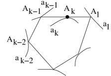
Proposition 2.16

Let $a_{1},\dots,a_{k}$ and $U$ be as above. Then $U$ contains no $k$-gon $A_{1}\dots A_{k}$ with the following properties:

- each pair of neighbor vertices correspond to distinct points, and no vertex is a marked point;

- there exists a unique $s\in\{1,\dots,k\}$ such that the line $A_{s}A_{s+1}$ is tangent to the curve $a_{s}$ at $A_{s}$, and the latter curve is not a line, see Fig.5.

Remark 2.17

A real version of Proposition 2.16 is contained in [7] (lemma 56, p.315 for $k=4$, and its generalization (lemma 67, p.322) for higher $k$).

Figure 5: Impossible degeneracy of simple tangency: $s=k$.

Proof.

Suppose the contrary: there exists a $k$-gon $A_{1}\dots A_{k}\in U$ as above. Without loss of generality we consider that $s=k$. Moreover, without loss of generality we can and will assume that the above tangency is quadratic: the quadrilaterals with a tangency vertex $A_{s}\in\hat{a}_{s}$ form a holomorphic curve in $U$ with variable $A_{s}$. For every $j=1,\dots,k$ the reflection with respect to the local branch of the curve $a_{j}$ at $A_{j}$ induces a mapping in the space $\mathbb{CP}^{2*}$ of projective lines. More precisely, for every $j\neq k$ it induces a germ of biholomorphic mapping $\psi_{j}:(\mathbb{CP}^{2*},A_{j}A_{j-1})\to(\mathbb{CP}^{2*},A_{j+1}A_{j})$, since the line $A_{j}A_{j-1}$ is transverse to $T_{A_{j}}a_{j}$ for these $j$. On the other hand, the germ $\psi_{k}$ is double-valued, with branching locus being the family of lines tangent to $a_{k}$. Indeed, the image of a line close to $A_{k}A_{k-1}=T_{A_{k}}a_{k}$ under the reflection from the curve $a_{k}$ at their intersection point depends on choice of the intersection point. The latter intersection point is a double-valued function with the above branching locus. The product $\psi_{k}\circ\dots\circ\psi_{1}$ should be identity on an open set accumulating to the line $A_{k}A_{1}$, since $A_{1}\dots A_{k}$ is a limit of an open set of $k$-periodic orbits. But this is impossible, since the product of a biholomorphic germ $\psi_{k-1}\circ\dots\circ\psi_{1}$ and a double-valued germ $\psi_{k}$ cannot be identity. The proposition is proved. ∎

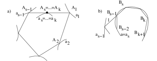
Proposition 2.18

Let $a_{1},\dots,a_{k}$ and $U$ be as at the beginning of the subsection. Then $U$ contains no $k$-gon $A_{1}\dots A_{k}$ with the following properties:

1) each its vertex is not a marked point of the corresponding mirror;

2) there exist $s,r\in\{1,\dots,k\}$, $s<r$ such that $a=a_{s}=a_{s+1}=\dots=a_{r}$, $A_{s}=A_{s+1}=\dots=A_{r}$, and $a$ is not a line;

3) For every $j\notin\mathcal{R}=\{s,\dots,r\}$ one has $A_{j}\neq A_{j\pm 1}$ and the line $A_{j-1}A_{j}$ is not tangent to $a_{j}$ at $A_{j}$, see Fig.6a.

Figure 6: Coincidence of subsequent vertices and mirrors: $r=k$.

Proof.

The proof of Proposition 2.18 repeats the above proof with some modifications. For simplicity we give the proof only in the case, when the complement $\{1,\dots,k\}\setminus\mathcal{R}$ is non-empty. In the opposite case the proof is analogous and is a straightforward complexification of the arguments from [21]. Without loss of generality we consider that $r=k$, then $s\geq 2$, and we will assume that the mirror $a=a_{s}$ has quadratic tangency with $T_{A_{s}}a_{s}$, as in the above proof. Consider the germs $\psi_{j}$ from the above proof. Set

$$\phi=\psi_{s-1}\dots\psi_{1},\ \psi=\psi_{k}\dots\psi_{s}.$$

A holomorphic branch of the product $\psi\circ\phi$ following an open set of $k$-periodic orbits accumulating to $\pi_{a_{1}}(A_{1})\dots\pi_{a_{k}}(A_{k})$ should be identity, as in the above proof. The germ $\phi$ is biholomorphic. We claim that the germ $\psi$ is double-valued on a small neighborhood of the line $A_{s-1}A_{s}$. Indeed, a line $l$ close to $A_{s-1}A_{s}=T_{A_{s}}a_{s}$ and distinct from the latter intersects the local branch $a_{A_{s}}$ at two distinct points close to $\pi_{a}(A_{s})$. Let us choose one of them and denote it $B_{s}\in l\cap a_{A_{s}}$, and denote $B_{s-1}$ the other intersection point. Then the ordered pair $(B_{s-1},B_{s})$ extends to a unique orbit $B_{s-1}\dots B_{k+1}$ of length $k+3-s$ of the billiard on the local branch $a_{A_{s}}$, see Fig.6b. The line $l^{*}=B_{k}B_{k+1}$ is the image of the line $l$ under a branch of the mapping $\psi$. For different choices of the intersection point $B_{s}$ we get different lines $l^{*}$. Indeed let us fix the above $B_{s}$ and complete the above orbit to the orbit $B_{2s-k-2}\dots B_{k+1}$ on $a_{A_{s}}$ of length $2k+4-2s$. Then the output line $l^{*}$ corresponding to the other intersection point $B_{s-1}$ is the line $B_{2s-k-1}B_{2s-k-2}$, by definition. It is distinct from the line $B_{k}B_{k+1}$ for an open set of lines $l$, analogously to arguments from [21]. This together with the double-valuedness of the intersection point $l\cap a_{A_{s}}$ proves the double-valuedness of the above germ $\psi$. Each $k$-periodic orbit $B_{1}\dots B_{k}$ corresponding to a point in $U_{0}$ close to $A_{1}\dots A_{k}$ contains a sub-orbit $B_{s}\dots B_{k}$ on $a_{A_{s}}$ as above. This implies that the product of the above biholomorphic germ $\phi$ and double-valued germ $\psi$ should be identity, – a contradiction. This proves the proposition. ∎

Corollary 2.19

There are no 4-reflective planar algebraic billiards with a pair of coinciding neighbor mirrors.

Proof.

Suppose the contrary: there exists a 4-reflective planar algebraic billiard $a$, $b$, $b$, $d$. Then $b$ cannot be a line, since otherwise, there would exist no 4-periodic orbit $ABCD$: by Definition 1.3, the lines $AB\neq b$ and $BC=b$ should be symmetric with respect to the non-isotropic line $b$, which is impossible. Let $U\subset\hat{a}\times\hat{b}\times\hat{b}\times\hat{d}$ denote the 4-reflective set. It is two-dimensional and contains at least one irreducible algebraic curve $\Gamma$ consisting of quadrilaterals $ABBD$ with coinciding variable vertices $B=C$, by epimorphicity of the projection $U\to\hat{b}\times\hat{b}$ (Proposition 2.14). Let us fix the above $\Gamma$. There are three possible cases:

Case 1): $A\not\equiv B$, $D\not\equiv B$ on $\Gamma$. Then $AB\equiv BD\equiv T_{B}b\not\equiv T_{A}a,T_{D}d$, since the set of lines tangent to two algebraic curves at distinct points is finite. This implies that $A\not\equiv D$ and a generic quadrilateral $ABBD\in\Gamma$ represents a counterexample to Proposition 2.18 with $s=2$, $r=3$.

Case 2): $A\equiv B$, $D\not\equiv B$ on $\Gamma$. Then we get a contradiction to Proposition 2.18 with $s=1$, $r=3$. The case $A\not\equiv B$, $D\equiv B$ is symmetric.

Case 3): $A\equiv B\equiv C\equiv D$ on $\Gamma$. Then we get a contradiction to Proposition 2.18 with $s=1$, $r=4$. Corollary 2.19 is proved. ∎

Corollary 2.20

Let $a$, $b$, $c$, $d$ be a 4-reflective analytic planar billiard, and let $b$ be not a line. Let $U\subset\hat{a}\times\hat{b}\times\hat{c}\times\hat{d}$ be the 4-reflective set. Let $ABCD\in U$ be such that $A\neq B$, $B\neq C$, the line $AB=BC$ is tangent to the curve $b$ at $B$ and is not isotropic. Then

- either $AD=DC$ is tangent to the curve $d$ at $D$, $\pi_{a}(A)=\pi_{c}(C)$, $a=c$ and the corresponding local branches coincide, i.e., $a_{A}=c_{C}$ (see Convention 2.11): “opposite tangency connection”, see Fig.7a;

- or $\pi_{d}(D)$ is a cusp of the branch $d_{D}$ and the tangent line $T_{D}d$ is not isotropic: “tangency–cusp connection”, see Fig.7b.

Figure 7: Opposite degeneracy to tangency vertex: tangency or cusp.

Proof.

Let $\mathcal{T}\subset U$ denote an irreducible germ at $ABCD$ of analytic curve consisting of quadrilaterals $A^{\prime}B^{\prime}C^{\prime}D^{\prime}$ such that $A^{\prime}B^{\prime}=T_{B^{\prime}}b$. Then $A^{\prime}B^{\prime}\equiv B^{\prime}C^{\prime}\equiv T_{B^{\prime}}b$ on $\mathcal{T}$, hence $A^{\prime}$, $B^{\prime}$, $C^{\prime}$ vary along the curve $\mathcal{T}$. Without loss of generality we consider that

(i) the line $AB=BC$ has quadratic tangency with the curve $b$ at $B$ and is transverse to $a$ and $c$ at $A$ and $C$ respectively;

(ii) the points $A$, $B$, $C$ are finite and not marked;

(iii) $A\neq D$ and $D\neq C$;

(iv) the germ at $ABCD$ of the projection $\pi_{a,b}:U\to\hat{a}\times\hat{b}$ is open.

One can achieve this by deforming the quadrilateral $ABCD$ along the curve $\mathcal{T}$. Indeed, it is easy to achieve conditions (i) and (ii). Condition (iv) can be achieved, since the projection $\pi_{a,b}$ is open at a generic point of the curve $\mathcal{T}$. Indeed, it is a submersion on an open and dense subset in $U$ (Proposition 2.14). Hence, it is open outside at most countable union of curves contracted to points by $\pi_{a,b}$ (if any), while $\Gamma$ is not contracted. Condition (iii) can be achieved, since $A^{\prime}\not\equiv D^{\prime}$ and $D^{\prime}\not\equiv C^{\prime}$ on $\mathcal{T}$. Indeed, if, e.g., $A^{\prime}\equiv D^{\prime}$, then the one-parameter family of lines $A^{\prime}B^{\prime}$ would be tangent to both curves $a$ and $b$ at distinct points $\pi_{a}(A^{\prime})$, $\pi_{b}(B^{\prime})$, which is impossible. Then either $D^{\prime}=D$ is a marked point (cusp or isotropic tangency) that is constant on the curve $\mathcal{T}$, or the line $A^{\prime}D^{\prime}=D^{\prime}C^{\prime}$ is tangent to $d$ at $D^{\prime}$ for every $A^{\prime}B^{\prime}C^{\prime}D^{\prime}\in\mathcal{T}$. This follows from conditions (i)–(iv), Proposition 2.16 and the discreteness of the set of marked points in $\hat{d}$.

Case 1): $D^{\prime}=D$ is a marked point that is constant on $\mathcal{T}$. Let $D$ be an isotropic tangency point. Then one of the lines $A^{\prime}D$ or $DC^{\prime}$ identically coincides with the isotropic tangent line $T_{D}d$ (Proposition 2.14). Hence, either $A^{\prime}$, or $C^{\prime}$ is constant on the curve $\mathcal{T}$, which is impossible, see the beginning of the proof. Thus, $\pi_{d}(D)$ is a cusp and the tangent line $T_{D}d$ is not isotropic.

Case 2): $D$ is not a marked point, the line $AD=DC$ is tangent to $d$ at $D$, and this holds in a neighborhood of the quadrilateral $ABCD$ in the curve $\mathcal{T}$. In the case, when $\pi_{a}(A^{\prime})\equiv\pi_{c}(C^{\prime})$ on $\mathcal{T}$, one has $a_{A}=c_{C}$, and we are done. Let us show that the opposite case is impossible. Suppose the contrary. Then deforming the quadrilateral $ABCD$ along the curve $\mathcal{T}$, one can achieve that in addition to conditions (i)–(iv), one has $A\neq C$. Thus, the line $A^{\prime}C^{\prime}$ is identically tangent to both curves $b$ and $d$ at $B^{\prime}$ and $D^{\prime}$ respectively along the curve $\mathcal{T}$. Therefore, $B^{\prime}\equiv D^{\prime}$, $b=d$ and the tangent line $A^{\prime}B^{\prime}$ to $b$ is orthogonal to both $T_{A^{\prime}}a$ and $T_{C^{\prime}}c$ identically on $\mathcal{T}$ (reflection law). Let us fix a local parameter $t$ on the curve $b$ in a neighborhood of the point $B$. Consider a quadrilateral $A_{1}B_{1}C_{1}D_{1}\in U_{0}\subset U\setminus\mathcal{T}$ close to $ABCD$. Then $A_{1}B_{1}\neq T_{B_{1}}b$ and $A_{1}B_{1}\neq A_{1}D_{1}$. Let $L_{1}$ ($R_{1}$) denote the line through $A_{1}$ ($C_{1})$ orthogonal to $T_{A_{1}}a$ (respectively, $T_{C_{1}}c$). These lines are tangent to $b$ at some points $B_{L,1}$ and $B_{R,1}$ respectively. Set $\varepsilon=t(B_{1})-t(B_{L,1})$. Without loss of generality we consider that the point $\pi_{d}(D)$ is finite, since $D^{\prime}\equiv B^{\prime}$ varies along the curve $\mathcal{T}$. We measure angles between lines in the finite affine chart $\mathbb{C}^{2}$. We show that the angle between the tangent lines $T_{B_{1}}b$ and $T_{D_{1}}b$ is of order $\varepsilon$ on one hand, and of order $O(\varepsilon^{2})$ on the other hand, as $\varepsilon\to 0$. The contradiction thus obtained will prove the corollary. We identify a point of the curve $b$ (or its normalization $\hat{b}$) with its $t$-coordinate. The angle between the lines $L_{1}$ and $A_{1}B_{1}$ is of order $\varepsilon^{2}$ (quadraticity of tangency). This and analogous statement for $C_{1}$ together with the reflection law at $A_{1}$, $C_{1}$ and $D_{1}$ imply the following asymptotics, as $\varepsilon\to 0$:

a) $\angle(A_{1}B_{1},A_{1}D_{1})=O(\varepsilon^{2})$, $\angle(C_{1}B_{1},C_{1}D_{1})=O(\varepsilon^{2})$;

b) $B_{1}-D_{1}=c\varepsilon(1+o(1))$, $c\neq 0$.

Let us prove statement b) in more detail. The lines $A_{1}B_{1}$ and $A_{1}D_{1}$ are symmetric with respect to the line $L_{1}$, hence $\angle(L_{1},A_{1}B_{1})\simeq-\angle(L_{1},A_{1}D_{1})$. They intersect the local branch $b_{B_{L,1}}$ at the points $B_{1}$ and $D_{1}$ respectively. This together with the quadraticity implies that $B_{1}-B_{L,1}\simeq\pm i(D_{1}-B_{L,1})$. The latter implies statement b) with appropriate constant $c\neq 0$. The angle $\angle(T_{B_{1}}b,T_{D_{1}}b)$ is an order $\varepsilon$ quantity, by statement b) and quadraticity. On the other hand, it is the angle between the symmetry lines for the pairs of lines $(A_{1}B_{1},B_{1}C_{1})$ and $(A_{1}D_{1},D_{1}C_{1})$ respectively. This together with statement a), which says that the latter pairs are “$O(\varepsilon^{2})$-close”, implies that the above angle should be also of order $O(\varepsilon^{2})$. The contradiction thus obtained proves the corollary. ∎

Corollary 2.21

Let in a 4-reflective complex algebraic planar billiard $a$, $b$, $c$, $d$ the mirror $b$ be not a line and $d$ have no cusps with non-isotropic tangent lines. Then $a=c$.

Proof.

There exists an irreducible algebraic curve $\mathcal{T}\subset U$ consisting of those quadrilaterals $ABCD$ with variable $B$ for which $AB=T_{B}b$: every 4-periodic billiard orbit can be deformed without changing the vertex $B$ to such a quadrilateral. Let us fix an $ABCD\in\mathcal{T}$ with $B\neq A,C$ and non-isotropic tangent line $T_{B}b$. Its vertex $D$ is not a cusp with non-isotropic tangent line, by assumption. Therefore, $a=c$, by Corollary 2.20. ∎

2.3 Case of a straight mirror

Here we apply the results of the previous subsection to classify the 4-reflective algebraic billiards with at least one mirror being a line.

Proposition 2.22

Let $a$, $b$, $c$, $d$ be a 4-reflective algebraic billiard in $\mathbb{CP}^{2}$ such that $a$ is a line. If some of the mirrors $b$ or $d$ is not a line, then $a=c$ and the curves $b$, $d$ are symmetric with respect to the line $a$, see Fig.1. If $a$, $b$, $d$ are lines, then $c$ is also a line, the lines $a$, $b$, $c$, $d$ pass through the same point, and the line pairs $(a,b)$, $(d,c)$ are sent one into the other by complex isometry with unit Jacobian, see Fig.2.

Proof.

We already know that $b\neq a$, $a\neq d$, by Corollary 2.19. Let us first consider the case, when one of the mirrors $b$, $d$, say $b$ is not a line. Let $U$ be the 4-reflective set, and let $\mathcal{T}\subset U$ be an irreducible algebraic curve as in the proof of Corollary 2.20: it consists of those quadrilaterals $ABCD$ with variable $B$, for which the line $AB$ is tangent to $b$ at $B$. For every $ABCD\in\mathcal{T}$ such that $B$ is not a marked point and $A,C\neq B,D$ either the point $\pi_{d}(D)$ is a cusp of the branch $d_{D}$ (the same for all $ABCD\in\mathcal{T}$), or the line $AD$ is tangent to $d$ at $D$. This follows from Corollary 2.20. The first, cusp case is impossible, by a projective duality argument. Indeed, if $D$ were constant along the curve $\mathcal{T}$, then the lines $AB$ with variable $B$ would intersect at one and the same point $B^{*}$ symmetric to $\pi_{d}(D)$ with respect to the line $a$ (the reflection law). On the other hand, for every $ABCD\in\mathcal{T}$ and any other $A^{\prime}B^{\prime}C^{\prime}D^{\prime}\in\mathcal{T}$ close to it the intersection point $AB\cap A^{\prime}B^{\prime}=T_{B}b\cap T_{B^{\prime}}b$ tends to $\pi_{b}(B)$, as $A^{\prime}B^{\prime}C^{\prime}D^{\prime}\to ABCD$. Therefore, $\pi_{b}(B)\equiv B^{*}$, hence $B\equiv const$, as $ABCD$ ranges in $\mathcal{T}$, – a contradiction. Thus, for every $ABCD\in\mathcal{T}$ the line $AD$ is tangent to $d$ at the point $D$. Finally, the family of tangent lines $AB$ to $b$ is symmetric to the family of tangent lines $AD$ to $d$ with respect to the line $a$. This implies that the curves $b$ and $d$ are also symmetric: the above argument shows that the intersection points $AB\cap A^{\prime}B^{\prime}$ and $AD\cap A^{\prime}D^{\prime}$ should be symmetric and tend to $\pi_{b}(B)$ and $\pi_{d}(D)$ respectively. One has $\pi_{a}(A)\equiv\pi_{c}(C)$ on $\mathcal{T}$, hence $a=c$ (Corollary 2.20). The first statement of Proposition 2.22 is proved. Now let us consider the case, when $a$, $b$ and $d$ are lines. Let us prove the second statement of the proposition. If $c$ were not a line, then $a$ would also haven’t been a line, being symmetric to $c$ with respect to the line $b$ (the first statement of the proposition), – a contradiction to our assumption. Therefore, $c$ is a line. The composition of reflections from the lines $a$, $b$, $c$, $d$ is identity as a transformation of the space $\mathbb{CP}^{2*}$ of projective lines (4-reflectivity). This together with the last statement of Example 1.8 proves the second statement of the proposition. ∎

Let us prove that every 4-reflective billiard with at least one straight mirror is of one of the types 1) or 2). If each mirror is a line and some of them coincide, then the billiard is of type 1). Indeed, in this case the coinciding mirrors are opposite (Corollary 2.19), say $a=c$, and $b$, $d$ are symmetric with respect to the line $a$, by the isometry of the pairs $(a,b)$ and $(d,c)$. Otherwise, a billiard with a straight mirror is of type either 1), or 2), by Proposition 2.22. This proves Theorem 1.11 in the case of straight mirror.

2.4 Complex confocal conics

Here we recall the classical notions of confocality and foci for complex conics. We extend Urquhart’s Theorem 1.10 and the characterization of ellipse as a curve with two given foci to complex conics (Theorem 2.25 and Proposition 2.32 respectively). Afterwards we state and prove Lemma 2.35 characterizing pairs of confocal complex conics in terms of their isotropic tangent lines. Lemma 2.35 and its proof are based on the classical relations between foci and isotropic tangent lines (Propositions 2.27 and Corollary 2.28).

Let $\mathcal{K}_{\mathbb{R}}$ ($\mathcal{K}$) denote the space of all the conics in $\mathbb{RP}^{2}$ ($\mathbb{CP}^{2}$) including degenerate ones: couples of lines. This is a 5-dimensional real (complex) projective space. One has complexification inclusion $\mathcal{K}_{\mathbb{R}}\subset\mathcal{K}$. Let $\mathcal{K}^{\prime}\subset\mathcal{K}$ denote the set of smooth (non-degenerate) complex conics. Consider the subset $\Lambda_{\mathbb{R}}\subset\mathcal{K}_{\mathbb{R}}\times\mathcal{K}_{\mathbb{R}}$ of pairs of confocal ellipses. Let

$$\Lambda\subset\mathcal{K}\times\mathcal{K}$$

denote the minimal complex projective algebraic set containing $\Lambda_{\mathbb{R}}$.

Remark 2.23

The projective algebraic set $\Lambda$ is irreducible and has complex dimension 6. It is symmetric, as is $\Lambda_{\mathbb{R}}$. The subset

$$\Lambda^{\prime}=(\Lambda\setminus\operatorname{diag})\cap\mathcal{K}^{\prime}\times\mathcal{K}^{\prime}\subset\Lambda$$

is Zariski open and dense. These statements follow from definition.

Definition 2.24

Two smooth planar complex conics are confocal, if their pair is contained in $\Lambda$.

Theorem 2.25

For every pair of distinct complex confocal conics $a$ and $b$ the complex billiard $a$, $b$, $a$, $b$ is 4-reflective.

Proof.

Consider the fibration $\pi:F\to\mathcal{K}^{2}$, $F\subset(\mathbb{CP}^{2})^{4}\times\mathcal{K}^{2}$: the $F$-fiber over a pair $(a,b)\in\mathcal{K}^{2}$ is the product $a\times b\times a\times b\subset(\mathbb{CP}^{2})^{4}$. Let $\Sigma\subset F$ denote the set of pairs $(ABCD,(a,b))\in F$ such that $ABCD$ is an interior point of the 4-periodic orbit set of the billiard $a$, $b$, $a$, $b$. Set

$$\Lambda^{\prime\prime}=\pi(\Sigma)\cap\Lambda^{\prime}\subset\Lambda^{\prime}.$$

For the proof of Theorem 2.25 it suffices to show that $\Lambda^{\prime\prime}=\Lambda^{\prime}$. The set $\Sigma$ is a difference of two analytic subsets in $F$, as in the proof of Proposition 2.14. The set $\Lambda^{\prime\prime}$ is constructible, by the latter statement and Remmert’s Proper Mapping Theorem (see, [9, p.46 of the Russian edition]). The set $\Lambda^{\prime\prime}$ contains a Zariski dense subset $\Lambda_{\mathbb{R}}\setminus\operatorname{diag}\subset\Lambda^{\prime}$, by Urquhart’s Theorem 1.10. Hence, $\Lambda^{\prime\prime}$ contains a Zariski open and dense subset in $\Lambda^{\prime}$. Now it suffices to show that the subset $\Lambda^{\prime\prime}\subset\Lambda^{\prime}$ is closed in the usual topology. That is, fix an arbitrary sequence $(a_{n},b_{n})\in\Lambda^{\prime\prime}$ converging to a pair of smooth distinct confocal conics $(a,b)$, and let us show that the billiard $a$, $b$, $a$, $b$ is 4-reflective. To do this, fix an arbitrary pair $(A,B)\in a\times b$ that satisfies the following genericity conditions: $A\neq B$; $A$ and $B$ are finite and not isotropic tangency points of the corresponding conics; the pair of lines symmetric to $AB$ with respect to the lines $T_{A}a$ and $T_{B}b$ intersect the union $a\cup b$ at eight distinct points that are not isotropic tangency points. Pairs $(A,B)$ satisfying the latter conditions exist and form a Zariski open subset in $a\times b$, since $a\neq b$. The pair $(A,B)$ is a limit of pairs $(A^{n},B^{n})\in a^{n}\times b^{n}$ extendable to periodic orbits $A^{n}B^{n}C^{n}D^{n}$ of the billiard $a^{n}$, $b^{n}$, $a^{n}$, $b^{n}$, since the latter pairs form a Zariski open dense subset in $a^{n}\times b^{n}$, by Proposition 2.14. After passing to a subsequence, the above orbits converge to a 4-periodic orbit $ABCD$ of the billiard $a$, $b$, $a$, $b$, by construction and genericity assumption. Thus, each pair $(A,B)$ from a Zariski open subset in $a\times b$ extends to a quadrilateral orbit, and hence, the billiard is 4-reflective. Theorem 2.25 is proved. ∎

Remark 2.26

In the above argument the assumption that $a\neq b$ is important. Otherwise, a priori it may happen that while passing to the limit, some neighbor vertices $A^{n}$ and $B^{n}$ of a 4-periodic orbit collide, and in the limit we get a degenerate 4-periodic orbit with coinciding neighbor vertices.

Proposition 2.27

([12, p.179], [3, subsection 17.4.3.1, p.334], goes back to Laguerre) For every smooth real conic (ellipse, hyperbola, parabola) each its focus lies in two transverse isotropic tangent lines to the complexified conic.

Corollary 2.28

[12, p.179] Every two complexified confocal real planar conics have the same isotropic tangent lines: a pair of transverse isotropic lines through each focus (with multiplicities, see the next remark).

Remark 2.29

For every conic $a\subset\mathbb{CP}^{2}$ and $C\in\mathbb{CP}^{2}\setminus a$ there are two distinct tangent lines to $a$ through $C$. But if $C\in a$, then $T_{C}a$ is the unique tangent line through $C$. We count it twice, since it is the limit of two confluenting tangent lines through $C^{\prime}\notin a$, as $C^{\prime}\to C$. If $C\in a$ is an isotropic point at infinity, then $T_{C}a$ is a double isotropic tangent line to $a$.

Corollary 2.30

Every smooth complex conic has four isotropic tangent lines with multiplicities.

Definition 2.31

The complex focus of a smooth complex conic is an intersection point of some its two distinct isotropic tangent lines.

Proposition 2.32

Let $P,Q\in\mathbb{CP}^{2}$ be an unordered pair of points that does not coincide with the pair of isotropic points at infinity. Let $a\subset\mathbb{CP}^{2}$ be a parametrized analytic curve distinct from an isotropic line such that for every $A\in a$ the lines $AP$ and $AQ$ are symmetric with respect to the line $T_{A}a$. Then the curve $a$ is either a conic with foci $P$ and $Q$, or a line with $P$ and $Q$ being symmetric with respect to $a$.

Proof.

None of the points $P$ and $Q$ is an isotropic point at infinity. Indeed, if $P=I_{1}$, then $Q=I_{2}$, by symmetry, – a contradiction to the assumption that $\{P,Q\}\neq\{I_{1},I_{2}\}$. The curve $a$ is a phase curve of the following double-valued singular algebraic line field $\lambda_{P,Q}$ on $\mathbb{CP}^{2}$: for every $A\in\mathbb{CP}^{2}$ the lines $AP$ and $AQ$ are symmetric with respect to the line $\lambda_{P,Q}(A)$. The singular set of the latter field is the union of the isotropic lines through $P$ and those through $Q$. Each its phase curve is either a conic with foci $P$ and $Q$, or the symmetry line of the pair $(P,Q)$. This follows from the same statement for real $P$ and $Q$ in the real plane, which is classical, and by analyticity in $(P,Q)$ of the line field family $\lambda_{P,Q}$. The proposition is proved. ∎

Definition 2.33

A transverse hyperbola is a smooth complex conic in $\mathbb{CP}^{2}$ transverse to the infinity line. A generic hyperbola is a smooth complex conic that has four distinct isotropic tangent lines.

Remark 2.34

The complexification of a real conic $a$ is a generic hyperbola, if and only if $a$ is either an ellipse with distinct foci, or a hyperbola. The complexification of a circle is a non-generic transverse hyperbola through both isotropic points $I_{1}$, $I_{2}$, with two double isotropic tangent lines at them intersecting at its center. Each generic hyperbola is a transverse one. Conversely, a transverse hyperbola is a generic one, if and only if it contains no isotropic points at infinity. A conic confocal to a transverse (generic) hyperbola is also a transverse (generic) hyperbola. A generic hyperbola (a complexified ellipse or hyperbola with distinct foci) has four distinct finite complex foci (including the two real ones).

Lemma 2.35

Two smooth conics $a$ and $b$ are confocal, if and only if one of the following cases takes place:

1) $a$ and $b$ are transverse hyperbolas with common isotropic tangent lines;

2) “non-isotropic parabolas”: $a$ and $b$ are tangent to the infinity line at a common non-isotropic point, and their finite isotropic tangent lines coincide;

3) “isotropic parabolas”: the conics $a$ and $b$ are tangent to the infinity line at a common isotropic point, have a common finite isotropic tangent line and are obtained one from the other by translation by a vector parallel to the latter finite isotropic tangent line.

The first step in the proof of Lemma 2.35 is the following proposition.

Proposition 2.36

Let $a$ be a generic hyperbola. A smooth conic $b$ is confocal to $a$, if and only if $a$ and $b$ have common isotropic tangent lines.

Proof.

Let $\mathcal{K}^{\prime\prime}\subset\mathcal{K}^{\prime}$ denote the subset of generic hyperbolas. Set

$$\widetilde{\Lambda}=\Lambda\cap(\mathcal{K}^{\prime\prime}\times\mathcal{K}^{\prime}).$$

Let $\mathcal{C}\subset\mathcal{K}^{\prime\prime}\times\mathcal{K}^{\prime}$ denote the subset of pairs of conics having common isotropic tangent lines. These are quasiprojective algebraic varieties. We have to show that $\mathcal{C}=\widetilde{\Lambda}$. Indeed, one has $\mathcal{C}\supset\widetilde{\Lambda}$, by Corollary 2.28 and minimality of the set $\Lambda$. For every quadruple $Q$ of distinct isotropic lines, two through each isotropic point at infinity, let $C_{Q}\subset\mathcal{K}^{\prime}$ denote the space of smooth conics tangent to the collection $Q$. In other terms, the conics of the space $C_{Q}$ are dual to the conics passing through the given four points dual to the lines in $Q$ in the dual projective plane. No triple of the latter four points lies in the same line. This implies that the space $C_{Q}$ is conformally-equivalent to punctured projective line. The space $\mathcal{C}$ is holomorphically fibered over the four-dimensional space of the above quadruples $Q$ with fibers $C_{Q}\times C_{Q}$. This implies that $\mathcal{C}$ is a 6-dimensional irreducible quasiprojective variety containing another 6-dimensional irreducible quasiprojective variety $\widetilde{\Lambda}$. The latter is a closed subset in the usual topology of the ambient set $\mathcal{C}$, by definition. Hence, both varieties coincide. The proposition is proved. ∎

Proof.

of Lemma 2.35. We will call a pair of conics tangentially confocal, if they satisfy one of the above statements 1)–3). First we show that every pair $(a,b)$ of confocal conics is tangentially confocal. Then we prove the converse. In the proof of the lemma we use the fact that every pair of confocal conics is a limit of pairs of confocal generic hyperbolas, since the latter pairs form a Zariski open and dense subset in $\Lambda$. This together with Proposition 2.36 implies that every two confocal conics have common isotropic tangent lines (with multiplicities).

For the proof of Lemma 2.35 we translate the tangential confocality into the dual language. Let $I_{1}^{*},I_{2}^{*}\subset\mathbb{CP}^{2*}$ be the dual lines to the isotropic points at infinity, set $p=\overline{\mathbb{C}}_{\infty}^{*}=I_{1}^{*}\cap I_{2}^{*}$. A pair of smooth conics $a$ and $b$ are confocal generic hyperbolas, if and only if the dual curves $a^{*}$ and $b^{*}$ pass through the same four distinct points $A_{11},A_{12}\in I_{1}^{*}$, $A_{21},A_{22}\in I_{2}^{*}$ (Proposition 2.36). Now let $(a,b)$ be a limit of pairs $(a_{n},b_{n})$ of confocal generic hyperbolas, let $A_{ij}^{n}\in I_{i}^{*}$ denote the above points of intersection $a_{n}^{*}\cap b_{n}^{*}$, and let $a$ be not a generic hyperbola. Let us show that one has some of cases 1)–3). Passing to a subsequence, we consider that the points $A_{ij}^{n}$ converge to some limits $A_{ij}\in a^{*}\cap I_{i}^{*}$. Then one of the following holds:

(i) One has $A_{ij}\neq p$ for all $(i,j)$. Then $p\notin a^{*},b^{*}$, hence $a$ and $b$ are transverse hyperbolas, and we have case 1).

(ii) One has $A_{11}=A_{21}=p$, $A_{12},A_{22}\neq p$, and the conics $a^{*}$ and $b^{*}$ are tangent to each other at the limit $p$ of colliding intersection points $A_{11}^{n},A_{21}^{n}\in a_{n}^{*}\cap b_{n}^{*}$. This implies that the curves $a$ and $b$ are as in case 2).

(iii) One has $p=A_{11}=A_{21}=A_{22}\neq A_{12}$ (up to permuting $I_{1}$ and $I_{2}$), and the conics $a^{*}$ and $b^{*}$ are tangent to each other with triple contact at the limit $p$ of three colliding intersection points $A_{ij}^{n}\in a_{n}^{*}\cap b_{n}^{*}$. The corresponding tangent line coincides with $I_{2}^{*}$, since the points $A_{21}^{n},A_{22}^{n}\in a_{n}^{*}\cap I_{2}^{*}$ collide. Therefore, the conics $a$ and $b$ are tangent to the infinity line at $I_{2}$ and have triple contact there between them, and they have a common finite isotropic tangent line $A_{12}^{*}$ through $I_{1}$. Below we show that then we have case 3).

(iv) All the points $A_{ij}$ coincide with $p$. Then a smooth conic $a^{*}$ should be tangent at $p$ to both transverse lines $I_{1}^{*}$ and $I_{2}^{*}$, analogously to the above discussion, – a contradiction. Hence, this case is impossible.

Proposition 2.37

Let two distinct smooth conics $a,b\subset\mathbb{CP}^{2}$ be tangent to the infinity line $\overline{\mathbb{C}}_{\infty}$ at a common point. Then they have at least triple contact there, if and only if they are obtained from each other by translation.

Proof.

One direction is obvious: if conics $a$ and $b$ tangent to $\overline{\mathbb{C}}_{\infty}$ are translation images of each other, then they have common tangency point with $\overline{\mathbb{C}}_{\infty}$ and at least triple contact there between them. The latter follows from the elementary fact that in this case they may have at most one finite intersection point, which is a solution of a linear equation. Let us prove the converse. Suppose they are tangent to the infinity line at a common point and have at least triple contact there. Let $A\in a$ and $B\in b$ be arbitrary two finite points with parallel tangent lines. The translation by the vector $AB$ sends the curve $a$ to a curve $a_{1}$ tangent to $b$ at $B$ that has at least triple contact with $b$ at infinity. If $a_{1}\neq b$, then their intersection index is at least 5, – a contradiction. Hence, $a_{1}=b$. This proves the proposition. ∎

Thus, in case (iii) $a$ and $b$ are translation images of each other, by Proposition 2.37, and have a common finite isotropic tangent line (hence, parallel to the translation vector). Therefore, we have case 3).

For every smooth conic $a$ let $C_{a}$ ($CT_{a}$) denote respectively the space of smooth conics confocal (tangentially confocal) to $a$. These are quasiprojective varieties. We have shown above that $C_{a}\subset CT_{a}$, and for the proof of the lemma it suffices to show that $CT_{a}=C_{a}$. In the case, when $a$ is a generic hyperbola, this follows from Proposition 2.36. Note that $dimC_{a}>0$, since this is true for a Zariski open dense subset in $\mathcal{K}$ of generic hyperbolas $a$ (see Proposition 2.36 and its proof) and remains valid while passing to limits. Moreover, the subset $C_{a}\subset\mathcal{K}^{\prime}$ is closed by definition. Fix a smooth conic $a$ that is not a generic hyperbola. Let us show that $CT_{a}$ is a punctured Riemann sphere. This together with the inclusion $C_{a}\subset CT_{a}$ and closeness will imply that $CT_{a}=C_{a}$ and prove the lemma. We will treat separately each one of cases 1)–3) (or an equivalent dual case (i)–(iii)).

Case 3) is obvious: the space $CT_{a}$ of images of the conic $a$ by translations parallel to a given line is obviously conformally equivalent to $\mathbb{C}$. Let us treat case 2)=(ii). In this case the dual curve $a^{*}$ intersects the union $I_{1}^{*}\cup I_{2}^{*}$ at exactly three distinct points: $A_{12}\in I_{1}^{*}$, $A_{22}\in I_{2}^{*}$ and $p=I_{1}^{*}\cap I_{2}^{*}=\overline{\mathbb{C}}_{\infty}^{*}$. The tangent line $l_{p}=T_{p}a^{*}$ is transverse to the lines $I_{j}^{*}=pA_{j2}$, $j=1,2$, since $a^{*}$ is a conic intersecting each line $I_{j}^{*}$ at two distinct points. The conics tangentially confocal to $a$ are dual to exactly those conics $b^{*}$ that pass through the points $A_{12}$, $A_{22}$, $p$ and are tangent to the line $l_{p}$ at $p$. The latter three points and line being in generic position, the space of conics $b^{*}$ respecting them as above is a punctured projective line. In case (i) the proof is analogous and is omitted to save the space. Lemma 2.35 is proved. ∎

Corollary 2.38

Let two confocal conics $a$ and $b$ be tangent to each other. Then each their tangency point lies on the infinite line, the corresponding tangent line is isotropic, and one of the following cases holds:

(i) single tangency point of quadratic contact; either the tangency point is isotropic and the tangent line is finite; or it is non-isotropic, and the tangent line is infinite;

(ii) two tangency points, which are the two isotropic points at infinity; the tangent lines are finite;

(iii) single tangency point of triple contact: an isotropic point at infinity, the tangent line is infinite.

Proof.

Let $a$ and $b$ be tangent confocal conics. All their common tangent lines are isotropic, since this is true for generic hyperbolas and remains valid after passing to limit. Case 1) of the lemma corresponds to Cases (i) (first subcase) or (ii) of the corollary. Case 2) of the lemma corresponds to Case (i), second subcase. Case 3) of the lemma corresponds to Case (iii) of the corollary. These statements follow from the proof of the lemma (the arguments on the points $A_{ij}$ of intersection of the dual conics) and the fact that a tangency of two curves corresponds to a tangency of the dual curves. For example, in Case 1) (or equivalently, case (i) from the proof of the lemma) a tangency point $O$ of the conics $a$ and $b$ corresponds to a common tangency point of the dual conics $a^{*}$ and $b^{*}$ with a line $I_{j}^{*}$, $j=1,2$. This implies that $O=I_{j}$. The other cases are treated analogously. ∎

2.5 Curves with property (I) of maximal isotropic tangency

In this subsection we describe the class of special rational curves having property (I) introduced below (Proposition 2.42 and Corollary 2.44). We show in Subsection 3.2 that mirrors of every 4-reflective algebraic billiard without lines belong to this class. These results will be used in Section 4.

Definition 2.39

We say that a planar projective algebraic curve $a$ that is not a line has property (I), if every its isotropic tangent line intersects its normalization $\hat{a}$ at a single point $A$, see Convention 2.11; the intersection index of the curve $\hat{a}$ with $T_{A}a$ at $A$ (see Definition 2.12) then equals the degree of the curve $a$.

Remark 2.40

Every conic has property (I). Corollary 2.44 below shows that the converse is not true. A curve $a$ that is not a line has property (I), if and only if its dual $a^{*}$ satisfies the following statement:

($I^{*}$) For every $j=1,2$ and $t\in a^{*}\cap I_{j}^{*}$ the germ $(a^{*},t)$ is irreducible, the line $T_{t}a^{*}$ is the only line through $t$ tangent to $a^{*}$, and $t$ is their unique tangency point.

Corollary 2.41

Each planar projective curve with property (I) has at least two distinct isotropic tangent lines.

Proof.

Let $a$ be a property (I) curve. Its isotropic tangent lines are dual to the points of non-empty intersection $a^{*}\cap(I_{1}^{*}\cup I_{2}^{*})$. Hence, the contrary to the corollary would imply that this intersection reduces to $s=I_{1}^{*}\cap I_{2}^{*}$. The germ $(a^{*},s)$ is irreducible (the above statement ($I^{*}$)), and hence is not tangent at $s$, say, to the line $I_{1}^{*}$. This implies that $a^{*}$ should intersect $I_{1}^{*}$ at some other point. The contradiction thus obtained proves the corollary. ∎

Proposition 2.42

Let a rational curve $a$ have property (I). Then

(i) either $a$ has at least three distinct isotropic tangency points: then it has no cusps, and at least one its isotropic tangency point is finite;

(ii) or it has exactly two distinct isotropic tangency points; then at least one of them is an isotropic point at infinity, and $a$ has no cusps except maybe for some of the two latter points.

Proof.

The curve $a$ has at least two distinct isotropic tangent lines, by the above corollary. The tangency points should be distinct, since the contrary would obviously contradict property (I).

Case 1): $a$ has at least three distinct isotropic tangency points $A$, $B$, $C$. At least one of them is finite. Indeed, otherwise $A,B,C\in\overline{\mathbb{C}}_{\infty}$, and some of them, say $A$ is not isotropic. Hence, the curve $a$ is tangent to the infinity line at $A$ and intersects it at $B\neq A$, – a contradiction to property (I). Fix arbitrary two isotropic tangency points, say $A$ and $B$. We show that the curve $a$ has no cusps distinct from them. Applying this to the other pairs $(A,C)$ and $(B,C)$ will imply that $a$ has no cusps at all and will prove (i). Let $l_{A}$ and $l_{B}$ denote the projective lines tangent to $a$ at $A$ and $B$ respectively. They intersect $a$ only at $A$ (respectively, $B$), by property (I). This implies that $l_{A}\neq l_{B}$ and $O=l_{A}\cap l_{B}\notin a$. Consider the projection $\pi:\hat{a}\to\mathbb{CP}^{1}$: the composition of the parametrization $\pi_{a}:\hat{a}\to a$ and the projection from the point $O$. Its global degree and its local degrees at its critical points corresponding to $A$ and $B$ are equal to the degree of the curve $a$ (property (I)). These are the only critical points, since they have maximal order and $a$ is rational. Hence, $a$ has no cusps distinct from $A$ and $B$. This together with the above discussion proves (i).

Case 2): $a$ has exactly two isotropic tangency points $A$ and $B$. Let us prove (ii). As is shown above, $a$ has no cusps distinct from $A$ and $B$. The dual curve $a^{*}$ intersects the union $I_{1}^{*}\cup I_{2}^{*}$ exactly at two distinct points $l_{A}^{*}$ and $l_{B}^{*}$. Thus, $a^{*}$ intersects one of the lines $I_{j}^{*}$, say $I_{1}^{*}$ at a unique point $t$. Then $a^{*}$ is tangent to $I_{1}^{*}$ at $t$ (irreducibility of the germ $(a^{*},t)$, by ($I^{*}$)). This implies that $I_{1}\in a$ and proves (ii) and the proposition. ∎

Definition 2.43

A system of isotropic coordinates on $\mathbb{C}^{2}$ is a system of affine coordinates with isotropic axes.

Corollary 2.44

In case (ii) of Proposition 2.42 one of the following holds (here $d$ is the degree of the curve $a$):

- either the curve $a$ is tangent to $\overline{\mathbb{C}}_{\infty}$ at an isotropic point at infinity and has another finite isotropic tangency point; then in appropriate isotropic coordinates the curve $a$ is given by the following parametrization:

$$x=t^{p},\ y=t^{d},\ t\in\overline{\mathbb{C}},\ 0<p<d;$$ (2.7)

- or the curve $a$ passes through the two isotropic points at infinity and in appropriate isotropic coordinates it is given by the following parametrization:

$$x=t^{-p},\ y=t^{q},\ t\in\overline{\mathbb{C}},\ p,q\geq 1,\ p+q=d.$$ (2.8)

In both formulas $p$ and $d$ are relatively prime. In particular, the curve $a$ is without cusps, if and only if it is a conic and in the above formulas $p=1$, $d=2$ and $p=q=1$ respectively.

Proof.

Recall that the curve $a^{*}$ intersects the union $I_{1}^{*}\cup I_{2}^{*}$ exactly at two distinct points, and one of the intersections $a^{*}\cap I_{j}^{*}$ is a single point, see the end of the above proof. At each point of intersection $a^{*}\cap I_{j}^{*}$ the germ of the curve $a^{*}$ is irreducible, see $(I^{*})$. Therefore, we have the following possibilities (up to permuting $I_{1}^{*}$ and $I_{2}^{*}$):

Case 1): $a^{*}$ passes through $s=I_{1}^{*}\cap I_{2}^{*}=\overline{\mathbb{C}}_{\infty}^{*}$, $s=a^{*}\cap I_{1}^{*}$, then $a^{*}$ is tangent to $I_{1}^{*}$ at $s$ (statement ($I^{*}$)), and $a^{*}$ intersects $I_{2}^{*}$ at a unique point $t$ different from $s$. Then $a$ is tangent to the infinity line at $I_{1}$ and has a finite isotropic tangent line $t^{*}$ through $I_{2}$. The line $T_{t}a^{*}$ does not contain $s$, since otherwise, $T_{t}a^{*}=ts=I_{2}^{*}$ and $I_{1}^{*}$ would be two distinct tangent lines to $a^{*}$ through $s$, – a contradiction to property $(I^{*})$. Hence, the dual $O=(T_{t}a^{*})^{*}$ to the line $T_{t}a^{*}$ is a finite point, and it lies in $t^{*}\cap a$ by duality. The composition of the parametrization $\pi_{a}:\hat{a}\to a$ with the projection $a\to\mathbb{CP}^{1}$ from the point $I_{1}$ is a branched covering $\pi:\hat{a}\to\mathbb{CP}^{1}$. Either it is bijective, or it has exactly two critical points $O$ and $I_{1}$, since $a$ has neither cusps distinct from them, nor finite tangent lines through $I_{1}$. Therefore, taking $t^{*}$ as the $x$-axis, $O$ as the origin and $OI_{1}$ as the $y$-axis, we get (2.7) after appropriate coordinate rescalings.

Case 2): $a^{*}$ intersects each line $I_{j}^{*}$ at a unique point $t_{j}$ and is tangent to $I_{j}^{*}$ there (by statement ($I^{*}$)), and $t_{j}\neq s$. Hence, $a$ passes through both isotropic points transversely to the infinity line. Taking isotropic coordinates centered at the intersection $t_{1}^{*}\cap t_{2}^{*}$, we get (2.8) after appropriate rescalings.

The parametrizations in (2.7) and (2.8) can be chosen bijective; then $p$ and $d$ are relatively prime. Hence, if $d\neq 2$, the curve $a$ has at least one cusp: either at an isotropic point at infinity, or at the origin (the latter may take place only in case (2.7)). The corollary is proved. ∎

2.6 Reflection correspondences: irreducibility and contraction

In what follows, for every irreducible non-linear germ $(a,A)$ of analytic curve in $\mathbb{CP}^{2}$ (or briefly, irreducible non-linear germ) its Puiseaux exponent (see Definition 2.9) will be denoted by $r_{a}=r_{a}(A)$. The main results of this subsection are the following lemma, proposition and corollary. They will be used in Subsection 3.2 in the proof of property (I) of mirrors of a 4-reflective billiard and coincidence of their isotropic tangent lines. Proposition 2.50 stated below will be used in their proofs and also in Section 4, where we show that the mirrors are confocal conics.

Lemma 2.45

Consider a pair of distinct non-linear irreducible germs $(a,A)$ and $(b,B)$, set $L=T_{A}a$. Let $L$ be isotropic and $B\in L$. Let $\Pi_{ab}\subset b\times a\times\mathbb{CP}^{2*}$ denote the germ at $(B,A,L)$ of two-dimensional analytic subset defined as follows: $(\tau,t,l)\in\Pi_{ab}$, if and only if $t\in l$ and either $(\tau,t)=(B,A)$, or $t=A$ and $l=L$, or the lines $t\tau$, $l$ are symmetric with respect to $T_{t}a$. (Thus, $\Pi_{ab}$ contains the curve $b\times A\times L$.) Let one of the following conditions hold:

(i) $A\neq B$;

(ii) $A=B$, but $L=T_{A}a\neq T_{B}b$;

(iii) $A=B$, $L=T_{A}a=T_{B}b$ and $A$ is an infinite point;

(iv) $A=B$ is a finite point, $L=T_{A}a=T_{B}b$ and

$$r_{b}(2-r_{a})<r_{a}.$$ (2.9)

Then the germ $\Pi_{ab}$ is irreducible.

Definition 2.46

We say that three irreducible algebraic curves $b,a,d\subset\mathbb{CP}^{2}$ form a reflection-birational triple, if they are not lines, $b\neq a$, $a\neq d$ and there exists a birational isomorphism $\psi_{a}:\hat{b}\times\hat{a}\to\hat{a}\times\hat{d}$ such that for a non-empty Zariski open set of pairs $(B,A)\in\hat{b}\times\hat{a}$ one has $\psi_{a}(B,A)=(A,D)$ and the lines $AB$ and $AD$ are symmetric with respect to the tangent line $T_{A}a$.

Proposition 2.47

Let $b$, $a$, $d$ be a reflection-birational triple, $L$ be an isotropic tangent line to $a$. For every their tangency point $A\in\hat{a}$ and every $B\in\hat{b}\cap L$ consider the germ $\Pi_{ab}$ constructed above for the local branches $a_{A}$ and $b_{B}$. Let there exist a tangency point $A\in\hat{a}$, $T_{A}a=L$, such that for every $B\in\hat{b}\cap L$ the corresponding germ $\Pi_{ab}$ is irreducible. Then the line $L$ intersects the curve $\hat{d}$ at a unique point $D$, and the transformation $\psi_{a}$ contracts the curve $\hat{b}\times A$ to the point $(A,D)$.

Corollary 2.48

Let $b$, $a$, $d$ be a reflection-birational triple, and let $L$ be an isotropic tangent line to $a$. Let there exist a tangency point $A\in\hat{a}$, $T_{A}a=L$, such that for every $B\in\hat{b}\cap L$ the local branches $a_{A}$ and $b_{B}$ satisfy one of the conditions (i)–(iv) from Lemma 2.45. Then the line $L$ intersects the curve $\hat{d}$ at a unique point $D$.

The lemma and the proposition are proved below. The corollary follows immediately from them.

Remark 2.49

If in the above condition (iv) inequality (2.9) does not hold, then the germ $\Pi_{ab}$ is not irreducible, and some its irreducible component does not contain the curve $b\times A\times L$. This statement will not be used in the paper. Its proof omitted to save the space follows arguments similar to the proof of Lemma 2.45 given below. The author does not know whether the statement of Proposition 2.47 holds in full generality, without requiring the irreducibility of all the germs $\Pi_{ab}$ corresponding to some $A$.

For the proof of Lemma 2.45 we introduce affine coordinates $(x,y)$ centered at $A$ so that $L$ is the $x$-axis. We fix an arbitrarily small $c>0$, and for every $t\in a$ we consider the cone $K_{t}=K_{c,t}\subset\mathbb{CP}^{2}$ saturated by the lines through $t$ with moduli of azimuths greater than $c$. We denote

$$K_{t}^{*}=K_{c,t}^{*}=\text{ the image of the cone }K_{t}=K_{c,t}$$

$$\text{ under the symmetry with respect to the line }T_{t}a.$$ (2.10)

We already know that the cone $K_{t}^{*}$ shrinks to $L$, as $t\to A$ (Proposition 2.7), thus each connected component of the intersection $K_{t}^{*}\cap b$ shrinks to $B$. We show (case by case) that for every $t$ close enough to $A$ each one of the latter components is simply connected. Thus, for those $t$ the complement $b_{t}=b_{c,t}=b\setminus K_{t}^{*}$ is connected, and it is the whole curve $b$ with small holes deleted; the latter holes shrink to $B$, as $t\to A$. Note that for every $Q\in b_{t}$ the line $Qt$ reflects from $T_{t}a$ to a line $l_{t}$ through $t$ with modulus of azimuth no greater than $c$. Moreover, each line $l_{t}$ through $t$ with azimuth less than $c$ corresponds to some $Q\in b_{t}$. Let us localize the analytic set $\Pi_{ab}$ by the inequality $|\operatorname{az}l|<c$ with small $c>0$. Then for every $t\in a$ close enough to $A$ the preimage of the point $t$ under the projection $\Pi_{ab}\to a$ is a connected holomorphic curve conformally projected onto $b_{t}\subset b$ that accumulates to the curve $b\times A\times L$, as $t\to A$. This implies the irreducibility of the germ $\Pi_{ab}$.

The most technical cases of Lemma 2.45 are cases (iii) and (iv), when the germs $(a,A)$ and $(b,B)$ are tangent to each other. In the proof of the lemma in those cases we use Proposition 2.50 stated and proved below that concerns the family of tangent lines to the curve $b$. It describes the asymptotic relation between the tangency point and the intersection points of the tangent line with the curve $a$. It will imply that in case (iii) with $r_{a}<r_{b}$ and in case (iv) the cone $K_{t}^{*}$ contains no tangent line to $b$. This in its turn implies the simple connectivity of the components of the intersection $b\cap K_{t}^{*}$. In case (iii) with $r_{a}\geq r_{b}$ we study the projections of the components of the intersection $K_{t}^{*}\cap b$ to the $x$-axis. We show that the projection of each component lies in a disk disjoint from $x(t)$. This together with the Maximum Principle implies that the minimal topological disk $U_{t}$ containing the component is disjoint from the vertical line $\{x=x(t)\}$. This together with the Maximum principle, now applied to the projection $U_{t}\to\mathbb{CP}^{1}$ from the point $t$ implies that the intersection component under question is simply connected.

Now let us pass to the proofs.

We consider parametrized curves (germs) and identify them with their parameter spaces (disks in $\mathbb{C}$). Let $(a,A)$ and $(b,B)$ be distinct tangent irreducible non-linear germs: $A=B=O$, $T_{A}a=T_{B}b=L$. Let $(x,y)$ be affine coordinates centered at $O$ such that $L$ is the $x$-axis. Set

$$T_{ab}=\{(t,\tau)\in a\times b\ |\ t\in T_{\tau}b\},\ v=x(t),\ u=x(\tau).$$

The subset $T_{ab}\subset a\times b$ represents a germ of one-dimensional analytic set at $(O,O)$. We consider its irreducible components and their projections to the product $L\times L$: both $t$ and $\tau$ are projected to $L$ along the $y$-axis. Each irreducible component defines two implicit multivalued functions:

- the function $u=u(v)$, whose graph is the image of the component under the above projection;

- the function $\alpha=\alpha(v)$: the azimuth of the tangent line $T_{\tau}b$.

We normalize the coordinates so that the curves $a$ and $b$ are graphs of functions

$$b=\{y=x^{r_{b}}(1+o(1))\};\ a=\{y=\sigma x^{r_{a}}(1+o(1))\};\ \sigma\neq 0.$$ (2.11)

Proposition 2.50

Let $a$, $b$ be two tangent irreducible non-linear germs of analytic curves at a point $O\in\mathbb{CP}^{2}$. Let the coordinates $(x,y)$, the number $\sigma$, the germ $T_{ab}$ and the functions $v$ and $u$ be as above. Then for every irreducible component of the germ $T_{ab}$ the corresponding implicit functions $u(v)$ and $\alpha(v)$ have asymptotic Puiseaux expansions at $0$ of the following possible types; for every given pair $(a,b)$ all the corresponding asymptotics are realized by appropriate irreducible components:

Case 1): $r_{a}>r_{b}$. Two possible asymptotics for every $(a,b)$:

$$u=sv(1+o(1)),\ s=\frac{r_{b}}{r_{b}-1},\ \alpha=r_{b}s^{r_{b}-1}v^{r_{b}-1}(1+o(1)),$$ (2.12)

$$u=sv^{\frac{r_{a}-1}{r_{b}-1}}(1+o(1)),\ s=(\frac{\sigma}{r_{b}})^{\frac{1}{r_{b}-1}},\ \alpha=\sigma v^{r_{a}-1}(1+o(1)).$$ (2.13)

Case 2): $r_{a}=r_{b}=r=\frac{p}{q}$, $p,q\in\mathbb{Z}$ are relatively prime. Then

$$u=s^{q}v(1+o(1)),\ \alpha=rs^{p-q}v^{r-1}(1+o(1));\ s^{p}(r-1)-rs^{p-q}+\sigma=0.$$ (2.14)

Case 3): $r_{a}<r_{b}$. Set $r_{g}=\frac{p_{g}}{q_{g}}$, as above, $g=a,b$. Then

$$u=s^{q_{b}}v^{\frac{r_{a}}{r_{b}}}(1+o(1)),\ s^{p_{b}}=\frac{\sigma}{1-r_{b}};\ \alpha=r_{b}s^{p_{b}-q_{b}}v^{\frac{r_{a}(r_{b}-1)}{r_{b}}}(1+o(1)).$$ (2.15)

Proof.

The germ $T_{ab}$ is given by zero set of an analytic function germ on $a\times b$ at $(O,O)$ that has the type $u^{r_{b}}(1+o(1))+r_{b}u^{r_{b}-1}(v-u)(1+o(1))-\sigma v^{r_{a}}(1+o(1))$ in the variables $u$ and $v$. Or equivalently, by an equation

$$(1-r_{b})u^{r_{b}}(1+o(1))+r_{b}u^{r_{b}-1}v(1+o(1))-\sigma v^{r_{a}}(1+o(1))=0$$ (2.16)

with the left-hand side being an analytic function of the parameters of the curves $a$ and $b$. An implicit function $u(v)$ corresponding to an irreducible component of the germ $T_{ab}$ is a solution to (2.16) that has Puiseaux expansion without free term. Hence, the restrictions to its graph of the three monomials $(1-r_{b})u^{r_{b}}$, $r_{b}u^{r_{b}-1}v$, $-\sigma v^{r_{a}}$ should satisfy the following statements as multivalued functions in $v$ after substitution $u=u(v)$:

- at least two of the above monomials have lower Puiseaux terms in $v$ with equal powers; we call them principal monomials; their sum is of smaller order, i.e., it starts with higher terms;

- the remaining monomial (if any) should be of smaller order than the principal ones.

In more detail, consider the Newton diagram in $\mathbb{R}^{2}$ of the above triple of monomials. That is, take the union of the translation images of the positive quadrant by the vectors $(r_{b},0)$, $(r_{b}-1,1)$, $(0,r_{a})$. The Newton diagram is its convex hull. Its edges are segments in its boundary that are not contained in the coordinate axes. For every irreducible component of the germ $T_{ab}$ the corresponding principal monomials should lie in the same edge of the Newton diagram. Vice versa, each edge is realized by an irreducible component. This is a version of a classical observation due to Newton.

Case 1): $r_{a}>r_{b}$. Then the Newton diagram has two edges: the segments $[(r_{b},0),\ (r_{b}-1,1)]$ and $[(r_{b}-1,1),\ (0,r_{a})]$. These edges correspond to asymptotics (2.12) and (2.13) respectively.

Case 2): $r_{a}=r_{b}$. Then there is a unique edge $[(r_{b},0),\ (0,r_{a})]$, the three above monomials lie there and are principal. This implies (2.14).

Case 3): $r_{a}<r_{b}$. We have one edge $[(r_{b},0),\ (0,r_{a})]$, the point $(r_{b}-1,1)$ is in the interior of the Newton diagram, the principal monomials are $(1-r_{b})u^{r_{b}}$ and $-\sigma v^{r_{a}}$. This implies (2.15). Proposition 2.50 is proved. ∎

Proof.

of Lemma 2.45. As it was shown above, for the proof of the lemma it suffices to prove that for every $t\in a$ close to $A$ each connected component of the intersection $K_{t}^{*}\cap b=K_{c,t}^{*}\cap b$ is simply connected. Let us prove this case by case. To do this, we consider the projection $\nu_{t}:b\to\overline{\mathbb{C}}_{t}=\mathbb{P}(T_{t}\mathbb{CP}^{2})$ of the curve $b$ from the point $t$. Note that the intersection $K_{t}^{*}\cap b$ is the preimage of a disk $D(t)=\nu_{t}(K_{t}^{*})\subset\overline{\mathbb{C}}_{t}$; the symmetry with respect to the line $T_{t}a$ sends the disk $D(t)$ to another disk that correspond exactly to the lines through $t$ with moduli of azimuths greater than $c$. Let $(x,y)$ be affine coordinates centered at $A$ with $L$ being the $x$-axis. We identify all the projective lines $\overline{\mathbb{C}}_{t}=\overline{\mathbb{C}}$ by translations and introduce the coordinate $z=\frac{y}{x}$ on $\overline{\mathbb{C}}_{A}$: $z(L)=0$. This induces coordinate $z$ on each $\overline{\mathbb{C}}_{t}$.

Case (i): $A\neq B$. Then there exist neighborhoods $U=U(B)\subset b$ and $V=V(A)\subset a$ such that for every $t\in V$ the image $\nu_{t}(U)\subset\overline{\mathbb{C}}$ lies in the unit disk $D_{1}$: if $\tau\in b$ is close to $B$ and $t\in a$ is close $A$, then the line $t\tau$ is close to $L=AB$. This together with the Maximum Principle applied to the projection $\nu_{t}:U\to D_{1}$ implies the simple connectivity of components of the intersection $K_{t}^{*}\cap b$.

Case (ii): $A=B$ but $T_{B}b\neq L$. Then for every $t\in a$ close enough to $A$ the cone $K_{t}^{*}$ contains no tangent lines to $b$ through $t$, since $K_{t}^{*}$ shrinks to the line $L$ transverse to $T_{B}b$, as $t\to A$. Therefore, the projection $\nu_{t}$ of each component of the intersection $K_{t}^{*}\cap b$ to the disk $D(t)$ is a branched covering either without critical points, or with exactly one critical point of maximal multiplicity. The latter happens exactly when the intersection component under question contains $B$ and the latter is a cusp of the curve $b$: this is the critical point. In both cases the component is obviously simply connected.

Case (iv): $A=B=O$ is a finite point, $T_{A}a=T_{B}b=L$, and $r_{b}(2-r_{a})<r_{a}$. We choose $(x,y)$ to be a finite affine chart. Let us show that for every $t\in a$ close to $O$ the cone $K_{t}^{*}$ contains no tangent line to the curve $b$, as in Case (ii). Indeed, the azimuths of all the lines forming the cone $K_{t}^{*}$ have uniform asymptotics $O((x(t))^{2(r_{a}-1)})$, by (2.2). On the other hand, the azimuths of the tangent lines to $b$ through $t$ are of order $(x(t))^{\mu}$, $\mu<2(r_{a}-1)$. Indeed, in the case, when $r_{a}\geq r_{b}$, one has $\mu\in\{r_{b}-1,\ r_{a}-1\}$, see (2.12)–(2.14), hence $\mu\leq r_{a}-1<2(r_{a}-1)$. In the case, when $r_{a}<r_{b}$, one has $\mu=\frac{r_{a}(r_{b}-1)}{r_{b}}$, by (2.15), and hence $\mu<2(r_{a}-1)$: this is equivalent to the inequality $r_{b}(2-r_{a})<r_{a}$ from the assumption. Thus, the azimuths of the tangent lines uniformly asymptotically dominate the azimuths of the lines forming the cone $K_{t}^{*}$. Hence, the cone $K_{t}^{*}$ contains no tangent lines, whenever $t$ is close enough to $O$, and all the components of the intersection $K_{t}^{*}\cap b$ are simply connected, as in Case (ii).

Case (iii): $A=B=O$ is an infinite point and $T_{A}a=T_{B}b=L$. Then the azimuths of the lines forming the cone $K_{t}^{*}$ have uniform asymptotics $p\frac{y(t)}{x(t)}(1+o(1))=p\sigma(x(t))^{r_{a}-1}$, where $p\in\{\frac{r}{2},\ 1,\ \frac{r^{2}}{2r-1}\}$, $r=r_{a}$, by (2.3); here $\sigma$ is the same, as in (2.11).

Subcase (iii a): $r_{a}<r_{b}$. Then the azimuths of the tangent lines to $b$ through $t$ are of order $(x(t))^{\mu}$, $\mu=\frac{r_{a}(r_{b}-1)}{r_{b}}>r_{a}-1$, see (2.15). Therefore, the cone $K_{t}^{*}$ contains no tangent lines to $b$, whenever $t$ is close enough to $O$, and we are done, as in Case (ii).

Subcase (iii b): $r_{a}\geq r_{b}$. The intersection points $\tau\in b\cap K_{t}^{*}$ satisfy the asymptotic equation

$$y(\tau)+p\frac{y(t)}{x(t)}(1+o(1))(x(t)-x(\tau))=y(t).$$ (2.17)

Substituting the expressions $y(\tau)=(x(\tau))^{r_{b}}(1+o(1))$ and $y(t)=\sigma(x(t))^{r_{a}}(1+o(1))$, $u=x(\tau)$, $v=x(t)$, we get

$$u^{r_{b}}(1+o(1))-p\sigma v^{r_{a}-1}u(1+o(1))+\sigma v^{r_{a}}(p-1+o(1))=0.$$ (2.18)

Claim 1. Let $r_{a}\geq r_{b}$. Then there exists a finite subset $S\subset\mathbb{C}$ depending only on $r_{a}$, $r_{b}$ and $\sigma$ such that the projection to the $x$-axis of the intersection $K_{t}^{*}\cap b$ lies in $o(v)=o(x(t))$- neighborhood of the subset $Sv\subset\mathbb{C}$, as $t\to O$. If there exists a family $\tau_{t}$ of intersection points such that $x(\tau_{t})=v(1+o(1))$ (along a sequence $t_{k}\to O$), then $r_{a}=r_{b}$ and $y(\tau_{t}))=y(t)(1+o(1))$.

Proof.

In the case, when $r_{a}>r_{b}$, all the solutions $u$ to (2.18) are $o(v)$. Indeed, otherwise, if there existed a family of solutions $u$ to (2.18) that is not $o(v)$ along a sequence of points $t\to O$, then the term $u^{r_{b}}$ in (2.18) would have dominated the rest of (2.18), which is obviously impossible. Let us now treat the case, when $r_{a}=r_{b}=r$. Consider the three monomials $u^{r}$, $-p\sigma v^{r-1}u$ and $(p-1)\sigma v^{r}$ in the left-hand side of (2.18). In the case, when $p\neq 1$, their Newton diagram consists of one edge $[(r,0),(0,r)]$: the point $(1,r-1)$ lies on this edge. These are the principal monomials in a similar sense, as in the proof of Proposition 2.50. Therefore, if $p\neq 1$, then each solution to (2.18) has asymptotics $u=sv(1+o(1))$, with $s$ being a root of polynomial depending on $r$, $p$ and $\sigma$, as in the same proposition. The number $p$ being a three-valued function in $r$, we get a triple of polynomials depending on $r$ and $\sigma$. This proves the claim for the union $S$ of their roots. Let now $p=1$: then the third monomial vanishes. For every family of solutions $u=u(v)$ to (2.18) one has $u=O(v)$: otherwise, the monomial $u^{r}$ would have dominated the rest of the left-hand side in (2.18) along a subsequence $t_{k}\to O$, which is impossible, as above. Substituting $p=1$ and $u=O(v)$ to (2.18) yields that the expression $u^{r}-\sigma v^{r-1}u$ should be of order $o(v^{r})$. This implies that each family of solutions $u=u(v)$ to (2.18) has asymptotics either $u=o(v)$, or $u=v(s+o(1))$ with $s=\sigma^{\frac{1}{r-1}}$. This implies the first statement of the claim with $S$ consisting of zero and all the numbers $\sigma^{\frac{1}{r-1}}$. Let now there exist a family of solutions $u=v(1+o(1))$ to (2.18), i.e., there exist a family of solutions $\tau$ to (2.17) with $x(\tau)=x(t)(1+o(1))$. Then $r_{a}=r_{b}$, by the above discussion, and $y(\tau)=y(t)(1+o(1))$, by (2.17). This proves the claim. ∎

Given a family $U_{t}$ of connected components of the intersection $K_{t}^{*}\cap b$, let us prove their simple connectivity, whenever $t$ is close enough to $O$. Let $V_{t}\subset b$ denote the minimal topological disk containing $U_{t}$. Without loss of generality we consider that there exists an $s\in S$ such that for every $t$ close enough to $O$ the projection of the domain $U_{t}$, and hence $V_{t}$ to the $x$-axis lies in $o(v)$-neighborhood of the point $sv$, passing to subsequence $t_{k}\to O$ (Claim 1). Let $s\neq 1$. Then the domain $V_{t}$ does not contain $v=x(t)$, whenever $t$ is close enough to $O$. Therefore, the image of its projection $\nu_{t}:V_{t}\to\overline{\mathbb{C}}_{t}=\mathbb{P}(T_{t}\mathbb{CP}^{2})$ from the point $t$ is contained in the affine chart $\mathbb{C}=\overline{\mathbb{C}}_{t}\setminus\{x=x(t)\}$. Hence, $U_{t}=V_{t}$ is simply connected, by the Maximum Principle, as in Case (i). Let now $s=1$. We claim that then $U_{t}$ cannot be tangent to a line through $t$. Indeed, the $x$- and $y$- coordinates of all the points $\tau\in U_{t}$ are asymptotically equivalent to those of the point $t$, as $t\to O$, by the claim. Therefore, if there existed a $\tau\in U_{t}$ such that the line $t\tau$ is tangent to $b$ at $\tau$, then the azimuth of the tangent line would have been asymptotically equivalent to that of the line $T_{t}a$: both of them should be equivalent to $r\frac{y(t)}{x(t)}$. Thus, the cone $K_{t}^{*}$ would have contained a line with azimuth $r\frac{y(t)}{x(t)}(1+o(1))$, while we already know that the azimuths of all its lines should have uniform asymptotics $p\frac{y(t)}{x(t)}(1+o(1))$ with $p\in\{\frac{r}{2},\ 1,\ \frac{r^{2}}{2r-1}\}$, see (2.3). The latter three possible values of the number $p$ are distinct from $r$, since $r>1$. The contradiction thus obtained proves that in the case under consideration the component $U_{t}$ is not tangent to a line through $t$, and hence, is simply connected, as in Case (ii). This finishes the proof of simple connectivity of the components of the intersection $K_{t}^{*}\cap b$. Together with the discussion following Remark 2.49, this proves Lemma 2.45. ∎

Proof.

of Proposition 2.47. The mapping $\psi_{a}$ contracts the curve $\hat{b}\times A$ to a point $(A,D)$ with some $D\in\hat{d}\cap L$, by Proposition 2.7 and birationality. Fix an arbitrary $D\in\hat{d}\cap L$, and let us show that $\psi_{a}$ contracts the curve $\hat{b}\times A$ to $(A,D)$. This together with holomorphicity of the mapping $\psi_{a}$ on finitely punctured curve $\hat{b}\times A$ (isolatedness of indeterminacies) implies uniqueness of the intersection point $D$. Fix a line $l\neq L$ through $A$, a point $Q\in l\setminus A$ and consider the family of lines $l_{t}=Qt$ with $t\in\hat{a}$: $l_{t}\to l$, as $t\to A$. For every $t\in\hat{a}$ that is not an isotropic tangency point let $l_{t}^{*}$ denote the line symmetric to $l_{t}$ with respect to the tangent line $T_{t}a$. One has $l_{t}^{*}\to L$, by Proposition 2.7. Fix a family of intersection points $D_{t}\in l_{t}^{*}\cap\hat{d}$ that tend to $D$, as $t\to A$. Let $B_{t}\in\hat{b}\cap l_{t}$ denote the family of points such that $\psi_{a}(B_{t},t)=(t,D_{t})$: it exists and is unique by birationality. The family of pairs $(B_{t},t)\subset\hat{b}\times\hat{a}$ is obviously an algebraic curve, hence, there exists a limit $B=\lim_{t\to A}B_{t}\in\hat{b}\cap l$. If $B\neq A$, then $AB=l\neq L$, $\psi_{a}$ is holomorphic at $(B,A)$, $\psi_{a}|_{\hat{b}\times A}\equiv D$ in a neighborhood of the pair $(B,A)$ (Proposition 2.7), and we are done. Let now $B=A$. The irreducible surface germ $\Pi_{ab}$ contains the germs at $(B,A,L)$ of analytic curves $\gamma=\{(B_{t},t,l_{t}^{*})\ |\ t\in a_{A}\}$ and $\Gamma=B\times A\times\mathbb{CP}^{1}$, where $\mathbb{CP}^{1}$ is the space of projective lines through the point $A$. The germ $\Pi_{ab}$ is smooth in the complement to the curve $\Gamma$. Consider the mapping $\mathcal{Q}:\Pi_{ab}\to\hat{a}\times\hat{d}$: $\mathcal{Q}(B^{\prime},A^{\prime},L^{\prime})=\psi_{a}(B^{\prime},A^{\prime})$. This is a well-defined holomorphic mapping on the complement $\Pi_{ab}\setminus\Gamma$, by birationality and isolatedness of indeterminacies of the mapping $\psi_{a}$. One has $\mathcal{Q}(x)\to(A,D)$, as $x\to(B,A,L)$. Indeed, as $x=(B^{\prime},A^{\prime},L^{\prime})\to(B,A,L)$, set $(A^{\prime},D^{\prime})=\mathcal{Q}(x)$, the points $D^{\prime}$ tend to the intersection $\hat{d}\cap L$. The germ $\Pi_{ab}$ being irreducible, there are arbitrarily small connected neighborhoods of the point $(B,A,L)$ in $\Pi_{ab}$, and their complements to $\Gamma$ are also connected. For every latter neighborhood $V$ and each $x=(B^{\prime},A^{\prime},L^{\prime})\in V\setminus\Gamma$ the line $L^{\prime}$ is close to $L$. Therefore, the corresponding point $D^{\prime}$ should stay in one and the same local branch intersecting $L$ of the curve $\hat{d}$, as $x$ ranges in $V\setminus\Gamma$. This implies that the limit of the point $D^{\prime}$ exists and lies in $L$, as $x\to(B,A,L)$. If $x\to(B,A,L)$ along the curve $\gamma$, then $D^{\prime}\to D$, by construction. Hence, $\mathcal{Q}(x)\to(A,D)$, as $x\to(B,A,L)$ in $\Pi_{ab}\setminus\Gamma$. The germ at $(B,A,L)$ of the curve $\hat{b}\times A\times L$ is contained in $\Pi_{ab}$, and $\mathcal{Q}$ contracts it to the point $(A,D)$, by Proposition 2.7 and the previous statement. Or equivalently, $\psi_{a}$ contracts $\hat{b}\times A$ to $(A,D)$. This proves the proposition. ∎

3 Rationality, property (I) and coincidence of isotropic tangent lines and opposite mirrors

In this section and in what follows we consider that $a$, $b$, $c$, $d$ is a 4-reflective billiard, and no its mirror is a line. In Subsection 3.1 we prove birationality of neighbor edge correspondence (Lemma 3.1) and deduce rationality of mirrors (Corollary 3.2) and description of the degenerate quadrilateral orbits with one of the vertices being a cusp with isotropic tangency (Corollary 3.4). In Subsection 3.2 we show that the mirrors have property (I), common isotropic tangent lines, and opposite mirrors coincide: $a=c$, $b=d$.

3.1 Birationality of billiard and rationality of mirrors.

Lemma 3.1

Let $U\subset\hat{a}\times\hat{b}\times\hat{c}\times\hat{d}$ be the 4-reflective set. There exists a unique birational isomorphism $\psi_{a}:\hat{b}\times\hat{a}\mapsto\hat{a}\times\hat{d}$ such that $\psi_{a}(B,A)=(A,D)$ for every $ABCD\in U$. In particular, the algebraic set $U$ is irreducible, the projection $U\to\hat{a}\times\hat{b}$ is birational and the curves $b$ and $d$ have equal degrees.

Proof.

The algebraic set $U$ is epimorphically projected onto $\hat{a}\times\hat{b}$ (Proposition 2.14), and its projection to $\hat{b}\times\hat{a}\times\hat{d}$ defines an algebraic correspondence $\psi_{a}:\hat{b}\times\hat{a}\to\hat{a}\times\hat{d}$: $\psi_{a}(B,A)=(A,D)$ for every $ABCD\in U$. Suppose the contrary to birationality: one of the mappings $\psi_{a}^{\pm 1}$, say, $\psi_{a}$ is multivalued on an open set. Then there exists an open subset $V\subset\hat{b}\times\hat{a}$ such that for every $(B,A)\in V$ there exist at least two distinct quadrilateral orbits $ABC_{1}D_{1}$ and $ABC_{2}D_{2}$ of the billiard $a$, $b$, $c$, $d$, where $C_{j}$ and $D_{j}$ depend analytically on $(B,A)$; $(C_{1},D_{1})\neq(C_{2},D_{2})$ on $V$. The latter immediately implies that $C_{1}\neq C_{2}$ and $D_{1}\neq D_{2}$ on $V$ (after shrinking $V$). Indeed, if $C_{1}\equiv C_{2}\equiv C$ but $D_{1}\neq D_{2}$ on $V$, then $CD_{1}\equiv CD_{2}\equiv D_{1}D_{2}\equiv AD_{1}\equiv AD_{2}$, since the lines $CD_{j}$ and $AD_{j}$ are the images of the lines $BC$ and $AB$ under the symmetries with respect to the lines $T_{C}c$ and $T_{A}a$ respectively. Thus, $A$, $C$ and $D$ are on the same line for an open set of quadrilateral orbits $ABCD$, which is impossible. The quadrilaterals $C_{1}D_{1}D_{2}C_{2}$ form an open set of 4-periodic orbits of the billiard $c$, $d$, $d$, $c$ with two pairs of coinciding neighbor mirrors, - a contradiction to Corollary 2.19. This proves Lemma 3.1. ∎

Corollary 3.2

Let $a$, $b$, $c$, $d$ be a 4-reflective algebraic billiard, and the curve $a$ be not a line. Then $b$ and $d$ are rational curves. Thus, the mirrors of a 4-reflective algebraic billiard are rational, if none of them is a line.

As it is shown below, Corollary 3.2 is immediately implied by Lemma 3.1 and the following well-known theorem from algebraic geometry. It is a part of the Indeterminacy Resolution Theorem for birational mappings.

Theorem 3.3

(implicitly contained in [9], p.546 of Russian edition). Let $\psi:S_{1}\to S_{2}$ be a birational isomorphism of smooth complex projective surfaces. Then each curve in $S_{1}$ contracted by $\psi$ to a point in $S_{2}$ is rational.

Proof.

of Corollary 3.2. It suffices to show that $b$ is rational, by symmetry. There exists an isotropic tangency point $A\in\hat{a}$, since $a$ is not a line. The birational isomorphism $\psi_{a}:\hat{b}\times\hat{a}\to\hat{a}\times\hat{d}$ from Lemma 3.1 contracts the fiber $\hat{b}\times A$ to a pair $(A,D)\in\hat{a}\times\hat{d}$ with $D\in T_{A}a$, by Proposition 2.7, as in the proof of Proposition 2.47. Therefore, the fiber $\hat{b}\times A\simeq\hat{b}$ is a rational curve (Theorem 3.3), and thus, so is $b$. Corollary 3.2 is proved. ∎

Corollary 3.4

Let $a$, $b$, $c$, $d$ be a 4-reflective algebraic billiard, and $U$ be its 4-reflective set. Let $D\in\hat{d}$ be a cusp with isotropic tangent line. Let $\Gamma\subset U$ be a parametrized analytic curve consisting of quadrilaterals $ABCD\in U$ with fixed $D$ and variable $A$ or $C$. Then $B\equiv const$ along $\Gamma$, and $B$ is a cusp of the same degree (see Footnote 4 in Subsection 1.2), as $D$.

Proof.

Let, e.g., $A$ vary along the curve $\Gamma$. Fix a quadrilateral $ABCD\in\Gamma$ with $A\neq B,D$ and $A$ being not a marked point ($A\not\equiv B$, by Corollary 2.19). Then the birational transformations $\psi_{a}^{\pm 1}$ are biholomorphic at $(B,A)$ and $(A,D)$ respectively. The biholomorphicity together with the reflection law imply that the intersection index of the variable line $AB$ with the local branch $b_{B}$ is equal to that of the variable line $AD$ with $d_{D}$, i.e., the degree of the cusp $D$. Thus, it is greater than one, and we have two possibilities: either $AB=T_{B}b$ and $B$ varies along the curve $\Gamma$; or $B\equiv const$ along $\Gamma$ and it is a cusp of the same degree, as $D$, and we are done. Suppose the contrary: the former, tangency case takes place. Then $B\not\equiv C$ along $\Gamma$ (Corollary 2.19), and we can and will consider that $B\neq C$ and the line $T_{B}b$ is not isotropic in our quadrilateral $ABCD$. Hence, $ABCD\notin U$, by Corollary 2.20 and since the tangent line $T_{D}d$ is isotropic. The contradiction thus obtained proves Corollary 3.4. ∎

3.2 Property (I) and coincidence of isotropic tangent lines and opposite mirrors

The main result of the present subsection is the following lemma.

Lemma 3.5

The curves $a$, $b$, $c$, $d$ have property (I) and common isotropic tangent lines, and $a=c$, $b=d$.

Proof.

Let us first prove property (I) and coincidence of isotropic tangent lines. To do this, it suffices to show that for every isotropic tangent line $L$ to any mirror each one of the curves $\hat{a}$, $\hat{b}$, $\hat{c}$, $\hat{d}$ intersects $L$ at a single point.

Step 1. Fix an isotropic tangent line $L$ to some mirror. Among the tangent branches to $L$ of the mirrors let us fix the one that either has infinite tangency point, or is smooth, or has the maximal possible Puiseaux exponent. Let this be, say, the local branch of the curve $a$ at a point $A\in\hat{a}\cap L$. The curves $b$, $a$ and $d$ taken in this or inverse order form a reflection-birational triple (Definition 2.46 and Lemma 3.1). For every $B\in\hat{b}\cap L$ the pair of germs $a_{A}$ and $b_{B}$ satisfy some of the conditions (i)–(iv) of Lemma 2.45: if $A=B$ is a finite point and $T_{B}b=L$, then inequality (2.9) follows from the assumption that either the germ $a_{A}$ is smooth (hence $r_{a}\geq 2$), or $r_{a}\geq r_{b}$. Therefore, the curve $\hat{d}$ intersects the line $L$ at a single point $D$ (Corollary 2.48), hence $T_{D}d=L$. Analogously, the curve $\hat{b}$ intersects the line $L$ at a unique point, by the above arguments with $b$ and $d$ interchanged.

Step 2. Let us prove that each one of the curves $\hat{a}$ and $\hat{c}$ intersects the line $L$ at a unique point. To do this, note that the curves $a$, $d$, $c$ taken in this or inverse order also form a reflection-birational triple, by Lemma 3.1.

Case 1): $D$ is either an infinite point, or a finite point that is not a cusp. Then some of the conditions (i)–(iv) of Lemma 2.45 holds for $(a,A)$, $(b,B)$ replaced by the local branches $d_{D}$ and $a_{A}$ respectively, as in Step 1. Therefore, the curve $\hat{c}$ intersects the line $L$ at a unique point, as in Step 1, and analogously so does $\hat{a}$, by symmetry.

Case 2): $D$ is a finite cusp. Consider a one-parametric family $\Gamma$ of quadrilaterals $A^{\prime}B^{\prime}C^{\prime}D\in U$ with the above fixed $D$ and variable $A^{\prime}\in\hat{a}$. Then $B^{\prime}\equiv const$ on $\Gamma$, and it is a cusp, by Corollary 3.4. Thus, for every $A^{\prime}\in a$ the lines $A^{\prime}B^{\prime}$ and $A^{\prime}D$ are symmetric with respect to the line $T_{A^{\prime}}a$ (reflection law). Therefore, $a$ is a conic with foci $B^{\prime}$ and $D$, by Proposition 2.32. Hence, it intersects the line $L$ at their unique tangency point $A$. Let us show that $a=c$. The conic $a$ has at least two distinct isotropic tangent lines $l_{1}$ and $l_{2}$, set $P=l_{1}\cap l_{2}$. Each of them intersects the curve $\hat{d}$ at a unique point, by Step 1. These intersection points are distinct, as are their tangent lines $l_{1}$, $l_{2}$, and $P\notin d$, by uniqueness. Consider the composition of the projection $\pi_{d}:\hat{d}=\overline{\mathbb{C}}\to d$ with the projection $d\to\overline{\mathbb{C}}=\mathbb{CP}^{1}$ from the point $P$. This is a rational mapping $\hat{d}=\overline{\mathbb{C}}\to\overline{\mathbb{C}}$ that has two distinct critical points with the maximal multiplicity: the intersection points $\hat{d}\cap l_{j}$, $j=1,2$. Therefore, it has no other critical points, and in particular, the curve $d$ has no cusps with non-isotropic tangent lines. Hence, $a=c$, by Corollary 2.21, thus $c$ is a conic tangent to $L$.

We have proved that the mirrors have property (I) and common isotropic tangent lines. Recall that a curve with property (I) has no cusps with non-isotropic tangent lines (Propositon 2.42 and Corollary 2.44). This together with Corollary 2.21 implies that $a=c$ and $b=d$. Lemma 3.5 is proved. ∎

Corollary 3.6

Let $a$, $b$, $a$, $b$ be a 4-reflective complex planar algebraic billiard, and no mirror be a line. Then for every $A\in\hat{a}\setminus b$ that is not an isotropic tangency point the collection of lines through $A$ tangent to $b$ (with multiplicities) is symmetric with respect to the tangent line $T_{A}a$.

Proof.

It suffices to prove the statement of the corollary for every $A\in\hat{a}$ lying outside the finite set formed by the isotropic tangency points in $\hat{a}$ and the intersection of the curve $\hat{a}$ with the union of the curve $b$, isotropic tangent lines to $b$ and the lines tangent to $b$ at the points of intersection $b\cap c$. The statement of the corollary remains valid after passing to limits. Fix an $A$ as above. For every $B\in\hat{b}$ such that $A\in T_{B}b$ the pair $(A,B)$ lifts to a quadrilateral $ABCD\in U$ with $AB=BC=T_{B}b$ (Proposition 2.14); one has $A\neq B$ and $B\neq C$, by construction. Then $AD=DC$ is the tangent line to $b$ symmetric to $AB$ with respect to the line $T_{A}a$, by Corollary 2.20 and since $b$ has no cusps with non-isotropic tangent lines, as at the end of the above proof. This proves the corollary. ∎

4 Quadraticity and confocality. End of proof of Theorem 1.11

Recall that we assume that in the 4-reflective billiard under consideration no mirror is a line. We have already shown that $a=c$, $b=d$ and they are two distinct rational curves with property (I) and common isotropic tangent lines. In the next subsection we prove that they are conics. Their confocality will be proved in the second subsection. The main tools we use here are Corollaries 2.44, 3.6 and Proposition 2.50.

4.1 Quadraticity of mirrors

Theorem 4.1

Let a pair of rational planar curves $a$ and $b$ different from lines form a 4-reflective billiard $a$, $b$, $a$, $b$. Then $a$ and $b$ are conics.

Theorem 4.1 is proved below. First we show that the mirrors have no cusp (the next lemma). Then we split the proof of Theorem 4.1 into three cases (Proposition 4.4), two of them will be treated in separate propositions.

Lemma 4.2

In the conditions of Theorem 4.1 none of the curves $a$ and $b$ has cusps.

In the proof of this lemma we use the following proposition.

Proposition 4.3

Let a rational curve in $\mathbb{CP}^{2}$ with property (I) have a cusp. Then it has either only one cusp, or two cusps. In the latter case its local branches at the cusps have distinct degrees.

Proof.

The curve under consideration has one of the normal forms (2.7) or (2.8) in appropriate isotropic coordinates on the finite plane $\mathbb{C}^{2}$. Consider, e.g., case (2.7): then $p$ and $d$ are relatively prime. Suppose the contrary: the curve has cusps both at the origin and at the infinity, and the corresponding local branches have equal degrees. The latter degrees are equal to $p>1$ and $d-p$ respectively. Hence, $p$ and $d=2p$ are not relatively prime, – a contradiction. Case (2.8) is treated analogously. ∎

Proof.

of Lemma 4.2. Suppose the contrary: say, the curve $b$ has a cusp $B$, let us denote its lifting to $\hat{b}$ also by $B$. Consider an irreducible algebraic curve $\Gamma$ consisting of quadrilaterals $ABCD\in U$ with fixed $B$ and variable $A$. Then $D\equiv const$ on $\Gamma$, and it is a cusp of the same degree, as $B$, by Corollary 3.4. Let us show that $B\neq D$. The contradiction thus obtained to Proposition 4.3 will prove the lemma. The curve $b$ has one of the normal forms (2.7) or (2.8), and each its cusp is either an isotropic point at infinity, or the origin. If $B$ is an isotropic point at infinity, then the lines $AD$, which are symmetric to $AB$ with respect to the line $T_{A}a$, should pass through the other isotropic point at infinity, and the latter obviously coincides with $D$; thus $B\neq D$. Otherwise, $B$ is the origin in the normal form coordinates: then one has case (2.7), and the curve $b$ is tangent to the infinity line. If $B=D$, then for every $A$ the line $AB$ is orthogonal to the tangent line $T_{A}a$. Hence $a$ is a complexified circle, and thus, is tangent to finite lines at both isotropic points at infinity. Therefore, the infinite tangent line to the curve $b$ is transverse to $a$, - a contradiction to the fact that $a$ and $b$ have common isotropic tangent lines. Hence, $B$ and $D$ are distinct cusps of equal degrees, – a contradiction to Proposition 4.3. This proves Lemma 4.2. ∎

Proposition 4.4

Let $a$, $b$ be distinct rational curves with property (I), common isotropic tangent lines and no cusps. Then one of the following holds:

Case 1): some isotropic line is tangent to $a$, $b$ at distinct finite points;

Case 2): $a$, $b$ are tangent at their common finite isotropic tangency point;

Case 3): $a$ and $b$ are tangent to each other at both isotropic points at infinity; then they are conics.

Proof.

Let us first assume that one of the curves, say $a$ has a finite isotropic tangency point $A_{0}$, set $L=T_{A_{0}}a$. Then $b$ is tangent to $L$ at some point $B_{0}$. If $A_{0}=B_{0}$, then we have case 2). Otherwise, $B_{0}\neq A_{0}$, hence $B_{0}\notin a$ (property (I) of the curve $a$). In this case $B_{0}$ cannot be infinite. Indeed, otherwise, $B_{0}$ would be an isotropic point at infinity and $L$ would be the unique tangent line to $b$ through $B_{0}$ (property (I) of the curve $b$). But there is another tangent line $L^{*}\neq L$ to $a$ through $B_{0}$, since $B_{0}\notin a$, $a$ has no cusps and by Riemann–Hurwitz Formula for the projection $a\to\mathbb{CP}^{1}$ from the point $B_{0}$. The line $L^{*}$ is isotropic and not tangent to $b$, by construction and property (I), – a contradiction to the coincidence of isotropic tangent lines of the curves $a$ and $b$. Thus, we have case 1). If each one of the curves $a$ and $b$ has no finite isotropic tangency point, then one has case 3) (Proposition 2.42 and Corollary 2.44). Then the curves are conics, by the same corollary and absence of cusps. This proves the proposition. ∎

Remark 4.5

For every $g=a,b$ and every isotropic tangency point $G\in g$ (which is not a cusp by Lemma 4.2) the Puiseaux exponent $r_{g}=r_{g}(G)$ equals the degree of the curve $g$, by property (I).

Proposition 4.6

Let a pair of distinct curves $a$ and $b$ that are not lines form a 4-reflective billiard $a$, $b$, $a$, $b$. Let there exist an isotropic line $L$ that is tangent to $a$ and $b$ at distinct finite points. Then $a$ and $b$ are conics.

Proof.

By symmetry, it suffices to prove that $a$ is a conic, i.e., $r_{a}=2$ (Remark 4.5). Let $A_{0}\neq B_{0}$ be respectively the tangency points of the line $L$ with $a$ and $b$. Then $A_{0}\notin b$ (property (I) of the curve $b$). There exists another line $l\neq L$ through $A_{0}$ that is tangent to $b$, as in the above proof. Fix isotropic coordinates $(x,y)$ on the finite plane $\mathbb{C}^{2}$ with the origin at $A_{0}$, the $x$-axis $L$ and $x(B_{0})=1$. For every $t\in a$ close to $A_{0}$ there exists a line $l_{t}^{*}$ tangent to $b$ through $t$ that tends to $l$, as $t\to A_{0}$. Its image $l_{t}$ under the symmetry with respect to $T_{t}a$ tends to $L$, and $\operatorname{az}(l_{t})=O(v_{t}^{2(r_{a}-1)})$, $v_{t}=x(t)$ (Proposition 2.4). On the other hand, the line $l_{t}$ should be tangent to $b$ (Corollary 3.6), and so is $L$. Therefore, the intersection point $B_{t}=l_{t}\cap L$ tends to a finite point $B_{0}\neq A_{0}$. Thus, $l_{t}$ is the line through the points $B_{t}=(\beta_{t},0)$, $\beta_{t}\to x(B_{0})=1$, and $t=(v_{t},\sigma v_{t}^{r_{a}}(1+o(1)))$, $\sigma\neq 0$. Hence, the azimuth $\operatorname{az}(l_{t})$ is of order $-y(t)\simeq-\sigma v_{t}^{r_{a}}$, but on the other hand, it is $O(v_{t}^{2(r_{a}-1)})$. Thus, $2(r_{a}-1)\leq r_{a}$ and $r_{a}=2$. Proposition 4.6 is proved. ∎

Proposition 4.7

Let a pair of distinct curves $a$ and $b$ that are not lines form a 4-reflective billiard $a$, $b$, $a$, $b$. Let they be tangent to each other at their common finite isotropic tangency point $O$. Then they are conics.

Proof.

Let $(x,y)$ be affine coordinates on the finite plane with the origin at $O$, and the tangent line $L=T_{O}a=T_{O}b$ be the $x$-axis. Let $r_{a}$ and $r_{b}$ be the Puiseaux exponents at $O$ of the curves $a$ and $b$ respectively (degrees, see Remark 4.5), $r_{a}\leq r_{b}$. Suppose the contrary: $r_{b}\geq 3$. Then there exists another line $l\neq L$ through $O$ that is tangent to $b$, since the projection $b\to\mathbb{CP}^{1}$ from $O$ has degree $r_{b}-1\geq 2$, $b$ has no cusps and by Riemann–Hurwitz Formula. For every $t\in a$ close to $O$ let $l_{t}^{*}$ be the tangent line to $b$ through $t$ such that $l_{t}^{*}\to l$, as $t\to O$. Its image $l_{t}$ under the symmetry with respect to the line $T_{t}a$ is also tangent to $b$, tends to $L$, and $\operatorname{az}(l_{t})=O(v_{t}^{2(r_{a}-1)})$, $v_{t}=x(t)$, as in the above proof. On the other hand, the latter azimuth should be a quantity of order $v_{t}^{\nu}$, $\nu=\frac{r_{a}(r_{b}-1)}{r_{b}}$, by Proposition 2.50. This is impossible, since $\nu<r_{a}\leq 2(r_{a}-1)$. Proposition 4.7 is proved. ∎

Proof.

of Theorem 4.1. Lemma 4.2 shows that the curves $a$ and $b$ have no cusps. Proposition 4.4 lists all the possible cases 1)-3). Propositions 4.6 and 4.7 respectively show that in cases 1) and 2) the curves are conics. In case 3) the curves are automatically conics. This proves Theorem 4.1. ∎

4.2 Confocality

We have shown that $a$ and $b$ are distinct conics with common isotropic tangent lines. Here we prove that they are confocal, by using confocality criterion given by Lemma 2.35. This will finish the proof of Theorem 1.11.

Case 1): one of the conics, say $a$ is transverse to the infinity line (i.e., a transverse hyperbola). Then $b$ is also a transverse hyperbola confocal to $a$, since it has the same isotropic tangent lines and by Lemma 2.35, case 1).

Case 2): both $a$ and $b$ are tangent to the infinity line, and $a$ is tangent to it at a non-isotropic point $A_{0}$. Then $b$ is also tangent to it at a non-isotropic point $B_{0}$, by the coincidence of isotropic tangent lines.

Claim 1. $A_{0}=B_{0}$.

Proof.

Suppose the contrary: $A_{0}\neq B_{0}$. Let $I_{1,2}=(1:\pm i:0)$ be the isotropic points at infinity. Then $A_{0}$, $B_{0}$, $I_{1}$, $I_{2}$ are four distinct points on the infinity line. Let us choose an affine chart $(x,y)$ with the origin $I_{1}$, the $x$-axis being the infinity line with $x=z$ there. Fix an arbitrary point $A\in a$ close to $A_{0}$. Let $p_{A}$ denote the tangent line to $b$ through $A$ at a point close to $B_{0}$: $p_{A}$ tends to the infinity line ($x$-axis), as $A\to A_{0}$. Let $p^{*}_{A}$ denote the line symmetric to $p_{A}$ with respect to the line $T_{A}a$.

Claim 2. The line $p_{A}^{*}$ tends to the infinity line, as $A\to A_{0}$.

Proof.

Let $x_{0}$, $x_{1}$, $x_{2}$ denote respectively the $x$-coordinates of the points of intersection of the $x$-axis with the lines $p_{A}$, $T_{A}a$ and $p_{A}^{*}$. Set $u=x(A_{0})$, $v=x(B_{0})$. One has $x_{0}x_{2}=x_{1}^{2}$ (reflection law and Proposition 2.4), and $x_{0}\to v$, $x_{1}\to u\neq v$, as $A\to A_{0}$. Therefore, $x_{2}\to w=\frac{u^{2}}{v}\neq u$. Thus, $p_{A}^{*}$ is the line through the points $A$ and $(x_{2},0)$, one has $(x_{2},0)\to(w,0)\neq A_{0}$, as $A\to A_{0}$. Hence, $p_{A}^{*}$ tends to the $x$-axis, i.e., $\overline{\mathbb{C}}_{\infty}$. This proves the claim. ∎

Thus, the line $p_{A}^{*}$ should be a tangent line to $b$ that tends to the infinity line, by Corollary 3.6 and the above claim. There are two tangent lines to $b$ through the point $A_{0}$: the infinity line and a finite line, since $A_{0}\notin b$. Thus, there are two tangent lines to $b$ through $A$: the line $p_{A}$ and a line with a finite limit, as $A\to A_{0}$. Therefore, $p_{A}=p_{A}^{*}$, thus $p_{A}$ is orthogonal to $T_{A}a$ for all $A$ close enough to $A_{0}$. In other words, every tangent line to $b$ close to the infinity line is orthogonal to the conic $a$ at both their intersection points. Hence, this is true for all the tangent lines to $b$, by algebraicity. Thus, for every point $A\in a$ there is only one tangent line to the conic $b\neq a$ through $A$, which is impossible. This proves Claim 1. ∎

Thus, the conics $a$ and $b$ have common isotropic tangent lines and are tangent to the infinity line at the same non-isotropic point, by Claim 1. This together with Lemma 2.35 implies that $a$ and $b$ are confocal.

Case 3): $a$ is tangent to the infinity line at an isotropic point, say $I_{1}$. Then $b$ is also tangent to the infinity line at $I_{1}$, since the conics $a$ and $b$ have common isotropic tangent lines. Recall that $a\neq b$.

Claim 3. The conics $a$, $b$ are tangent at $I_{1}$ with at least triple contact.

Proof.

Let $(x,y)$ be affine coordinates with the origin $I_{1}$, the $x$-axis $\overline{\mathbb{C}}_{\infty}$ with $x=z$ there such that $b=\{y=x^{2}(1+o(1))\}$, as $(x,y)\to(0,0)$. Then $a=\{y=\sigma x^{2}(1+o(1))\}$, $\sigma\neq 0$. We have to show that $\sigma=1$. For every $t\in a$ close to $I_{1}$ set $v_{t}=x(t)$. There are two tangent lines $p_{1,t}$ and $p_{2,t}$ to $b$ through $t$, and they tend to the $x$-axis, i.e., the infinity line, as $t\to I_{1}$. Their azimuths have asymptotics $2s_{j}v_{t}(1+o(1))$, $j=1,2$, where $s_{j}$ are the roots of the quadratic equation $s^{2}-2s+\sigma=0$, and their tangency points with $b$ have $x$-coordinates $u_{t}=s_{j}v_{t}(1+o(1))$ (Proposition 2.50). Therefore, the latter tangent lines intersect the $x$-axis at points with coordinates $x_{j}=\frac{s_{j}}{2}v_{t}(1+o(1))$, while the tangent line $T_{t}a$ intersects it at a point with coordinate $x_{0}=\frac{v_{t}}{2}(1+o(1))$ (Proposition 2.10). The pair of lines $p_{j,t}$ is symmetric with respect to the line $T_{t}a$ (Corollary 3.6). The symmetry cannot fix each $p_{j,t}$ for all $t$, since otherwise either two distinct lines $p_{1,t}$ and $p_{2,t}$ would be orthogonal to $T_{t}a$, or one of them would be tangent to both $a$ and $b$ for all $t$; none of the latter is possible. Thus, the symmetry permutes the above lines. Hence, $x_{1}x_{2}=x_{0}^{2}$ (Proposition 2.4), and thus, $s_{1}s_{2}=1$. On the other hand, $s_{1}s_{2}=\sigma$, thus, $\sigma=1$. The claim is proved. ∎

Claim 3 together with Proposition 2.37 imply that in our case the conics $a$ and $b$ are obtained one from the other by translation of the finite plane. This together with the coincidence of their finite isotropic tangent lines and Lemma 2.35 implies that $a$ and $b$ are confocal. Theorem 1.11 is proved.

5 Degenerate orbits of billiard on conics

Here we consider a 4-reflective billiard $a$, $b$, $a$, $b$ on pair of distinct confocal conics $a$, $b$ and prove the following classification of degenerate quadrilateral orbits. Note that smooth mirrors coincide with their normalizations.

Theorem 5.1

Let $U\subset a\times b\times a\times b$ be the 4-reflective set, and let $U_{0}\subset U$ be the subset of 4-periodic orbits. The complement $U\setminus U_{0}$ is the union of the following algebraic curves:

(i) the curve $\mathcal{T}_{a}$ consisting of quadrilaterals $ABCB\in a\times b\times a\times b$ with $A,C\neq B$, $AB=T_{A}a$, $CB=T_{C}a$ and all the single-point quadrilaterals $AAAA$, $A\in a\cap b$; $AB\not\equiv CB$ on each component of the curve $\mathcal{T}_{a}$;

(ii) the curve $\mathcal{T}_{b}$ defined analogously with $a$ and $b$ interchanged;

(iii) for every isotropic tangent line $L$ to $a$ and $b$ at points $A_{0}$ and $B_{0}$ respectively the curve $\Gamma_{ab}(L)$ consisting of quadrilaterals $A_{0}B_{0}AB$ with variable $A$ and $B$; the curve $\Gamma_{ab}$ is rational, and the natural projections $\Gamma_{ab}\to a$, $\Gamma_{ab}\to b$ to the positions of the variable vertices $A$ and $B$ are bijective;

(iv) three other rational curves $\Gamma_{bc}(L)$, $\Gamma_{cd}(L)$, $\Gamma_{da}(L)$ defined analogously to $\Gamma_{ab}(L)$ and consisting of quadrilaterals $AB_{0}A_{0}B$, $ABA_{0}B_{0}$ and $A_{0}BAB_{0}$ respectively with variable $A$ and $B$.

Each one of the curves $\mathcal{T}_{a}$ and $\mathcal{T}_{b}$ is

- elliptic, if $a$ and $b$ are not tangent to each other;

- rational with one transverse self-intersection, if $a$ and $b$ are quadratically tangent at a unique point;

- rational with one cusp of degree two, if $a$ and $b$ are tangent with triple contact;

- a union of two smooth rational curves, if $a$ and $b$ are tangent at two distinct points.

Proof.

Fix a quadrilateral $ABCD\in U\setminus U_{0}$. Let us show that it lies in the union of the above curves. If its vertices are not isotropic tangency points and every two neighbor vertices are distinct, then it lies in $\mathcal{T}_{a}\cup\mathcal{T}_{b}$, by Corollary 2.20. If it has an isotropic tangency vertex, then some its neighbor is also an isotropic tangency vertex (reflection law and coincidence of isotropic tangent lines of the conics $a$ and $b$). Therefore, given an isotropic line $L$ tangent to $a$ and $b$ at points $A_{0}$ and $B_{0}$ respectively, there exists a rational curve $\Gamma_{L}=\Gamma_{ab}(L)$ of quadrilaterals $A_{0}B_{0}AB\in U\setminus U_{0}$ with variable $A$ (see the proof of Corollary 3.2). Let us show that $B$ also varies along $\Gamma_{L}$. Indeed, in the contrary case, when $B\equiv const$ on $\Gamma_{L}$, one would have either $B\equiv A_{0}$, or the variable line $AB$ is reflected to the constant line $BA_{0}$ (which is thus isotropic and coincides with $T_{B}b$). In both cases $T_{B}b=L$, by coincidence of isotropic tangent lines of the conics $a$ and $b$. Hence, $B\equiv B_{0}$ on $\Gamma_{L}$. Therefore, $AB_{0}$ is orthogonal to $T_{A}a$ for every $A\in a$, and $a$ is a complex circle centered at $B_{0}$. By confocality, $b$ is also a complex circle centered at $B_{0}\in b$, which is obviously impossible. The contradiction thus obtained proves that both $A$ and $B$ vary along the curve $\Gamma_{L}$. The projection of the curve $\Gamma_{L}$ to the position of either $A$, or $B$ is bijective, by birationality (Lemma 3.1).

A priori, $ABCD$ may have yet another degeneracy: coinciding pair of neighbor vertices that are not isotropic tangency points. First we show that the quadrilaterals in $U$ with the latter degeneracy form a finite set of points $AAAA\in\mathcal{T}_{a}\cap\mathcal{T}_{b}$, $A\in a\cap b$. Then we prove the last statements of the theorem on the structure of the curves $\mathcal{T}_{a}$ and $\mathcal{T}_{b}$.

Proposition 5.2

Let $A=B\in a\cap b$ be an intersection point such that the line $T_{A}a$ is not isotropic. Then the line $T_{B}b$ is also not isotropic, and the 4-reflective set $U$ contains no algebraic curve of quadrilaterals $AACD$ with fixed $A=B$ and variable $C$ or $D$.

Proof.

The non-isotropicity of the tangent line $T_{B}b$ follows immediately from the coincidence of isotropic tangent lines to $a$ and $b$ (confocality). The line $T_{B}b$ is transverse to $a$, since each common tangent line to $a$ and $b$ is isotropic (see the proof of Corollary 2.38). Suppose the contrary to the second statement: there exists an algebraic curve $H\subset U$ consisting of quadrilaterals $AACD$, say, with variable $C$. Let $C^{*}$ denote the point of intersection $a\cap T_{A}b$ distinct from $A$. Then $H$ contains a quadrilateral $x=AAC^{*}D^{*}$ with $AC^{*}=T_{A}b$ and $C^{*}\neq A$. The quadrilateral $x$ may be deformed to a quadrilateral $A^{\prime}B^{\prime}C^{\prime}D^{\prime}\in U$ with $B^{\prime}C^{\prime}=T_{B^{\prime}}b$ and $A^{\prime}\neq B^{\prime},C^{\prime}$, – a contradiction to Corollary 2.20. The proposition is proved. ∎

Let $A$ be as in Proposition 5.2. The proposition immediately implies that the birational isomorphisms $\psi_{a}$, $\psi_{b}$ and their inverses are biholomorphic at $(A,A)$. Let us show that they send $(A,A)$ to $(A,A)$. Indeed, take a point $A^{\prime}\in a$, the two tangent lines to $b$ through $A^{\prime}$ and the tangency points $B^{\prime}$ and $D^{\prime}$. One has $A^{\prime}B^{\prime}A^{\prime}D^{\prime}\in\mathcal{T}_{b}$, and $B^{\prime},D^{\prime}\to A$, as $A^{\prime}\to A$. This together with biholomorphicity and Lemma 3.1 implies that $\psi_{a}(A,A)=\psi_{b}^{-1}(A,A)=(A,A)$, $AAAA\in\mathcal{T}_{b}$ and $AAAA$ is the only quadrilateral in $U$ with a pair of neighbor vertices coinciding with $A$. Similarly, $AAAA\in\mathcal{T}_{a}$.

Let us prove the last statement of Theorem 5.1 for the curve $\mathcal{T}_{a}$; the case of the curve $\mathcal{T}_{b}$ is symmetric. In the case, when the conics $a$ and $b$ are not tangent, the ellipticity of the curve $\mathcal{T}_{a}$ is classical, see [8]. Namely, the projection $q:\mathcal{T}_{a}\to b\simeq\overline{\mathbb{C}}$: $ABCB\mapsto B$ is a double covering over $\overline{\mathbb{C}}$, branching over the points of intersection $a\cap b$. If the conics are not tangent, then we have four distinct branching points, thus the curve $\mathcal{T}_{a}$ is elliptic by Riemann–Hurwitz Formula. The cases of tangent confocal conics are described by Corollary 2.38. In the case, when $a$ and $b$ are quadratically tangent at some point $O$, the curve $\mathcal{T}_{a}$ has two transversely intersected local branches through the point $(O,O)$. This easily follows from Proposition 2.50, see (2.14). Therefore, the projection $q$ does not branch at the double intersection $O$ and has only two branching points; thus the curve $\mathcal{T}_{a}$ is rational by Riemann–Hurwitz Formula. The case of two tangency points is treated analogously: the covering does not branch at all and has two univalent sheets bijectively projected to $\overline{\mathbb{C}}$. In the case of triple tangency we have two distinct branching points: the point $O$ and another branching point. The implicit function $A=A(B)$ defined by the curve $\mathcal{T}_{a}$ is double-valued in the neighborhood of the point $O$, and its both branches have unit derivative at $O$, by (2.14). This easily implies that the quadrilateral $OOOO$ corresponds to a degree two cusp of the rational curve $\mathcal{T}_{a}$. Theorem 5.1 is proved. ∎

6 Application: classification of 4-reflective real algebraic planar pseudo-billiards

Here by real analytic curve we mean a curve $a\subset\mathbb{RP}^{2}$ analytically parametrized by either $\mathbb{R}$, or $S^{1}$ that is not the infinity line. If a curve $a$ has singularities (cusps or self-intersections), we consider its maximal real analytic extension $\pi_{a}:\hat{a}\to a$, where $\hat{a}$ is either $\mathbb{R}$, or $S^{1}$, see [7, lemma 37, p.302]. The parametrizing curve $\hat{a}$ will be called here the real normalization. The affine plane $\mathbb{R}^{2}\subset\mathbb{RP}^{2}$ is equipped with Euclidean metric.

Definition 6.1

A real planar analytic (algebraic) pseudo-billiard is a collection of $k$ real irreducible analytic (algebraic) curves $a_{1},\dots,a_{k}\subset\mathbb{RP}^{2}$. Its $k$-periodic orbit is a $k$-gon $A_{1}\dots A_{k}$, $A_{j}\in a_{j}\cap\mathbb{R}^{2}$, such that for every $j=1,\dots,k$ one has $A_{j}\neq A_{j\pm 1}$, $A_{j}A_{j\pm 1}\neq T_{A_{j}}a_{j}$ and the lines $A_{j}A_{j-1}$, $A_{j}A_{j+1}$ are symmetric with respect to the tangent line $T_{A_{j}}a_{j}$. The latter means that for every $j$ the triple $A_{j-1}$, $A_{j}$, $A_{j+1}$ and the line $T_{A_{j}}a_{j}$ satisfy either usual, or skew real reflection law. For brevity, we then say that usual (skew) reflection law is satisfied at the vertex $A_{j}$. Here we set $a_{k+1}=a_{1}$, $A_{k+1}=A_{1}$, $a_{0}=a_{k}$, $A_{0}=A_{k}$. A real pseudo-billiard is called $k$-reflective, if it has an open set (i.e., a two-parameter family) of $k$-periodic orbits. The interior points of the set of $k$-periodic orbits will be called $k$-reflective orbits.

Remark 6.2

The complexification of every real $k$-reflective planar analytic pseudo-billiard is a $k$-reflective analytic complex planar billiard.

Theorem 6.3

A real planar algebraic pseudo-billiard $a$, $b$, $c$, $d$ is 4-reflective, if and only if it has one of the following types:

1) $a=c$ is a line, the curves $b,d\neq a$ are symmetric with respect to it;

2) $a$, $b$, $c$, $d$ are distinct lines through the same point $O\in\mathbb{RP}^{2}$, the line pairs $(a,b)$, $(d,c)$ are transformed one into the other by rotation around $O$ (translation, if $O$ is an infinite point);

3) $a=c$, $b=d$ and they are distinct confocal conics: either ellipses, or hyperbolas, or ellipse and hyperbola, or parabolas.

In every 4-reflective orbit the reflection law at each pair of opposite vertices is the same; it is skew for at least one opposite vertex pair.

Addendum 1. In Theorem 6.3, case 1) each 4-reflective orbit $ABCD$ has the same type, as at Fig.1: it is symmetric with respect to the line $a=c$ and the reflection law is skew at $A$ and $C$. In the subcase, when $b$, $d$ are lines parallel to $a$, the reflection law is usual at $b$ and $d$. In the subcase, when $b=d$ is a line orthogonal to $a$, the orbits are rhombi symmetric with respect to $a$ and $b$: the reflection law is skew at each vertex, see Fig.11a). If none of the latter subcases holds, then the billiard has both types of 4-reflective orbits $ABCD$: with usual reflection law at $B$, $D$ and with skew one.

Addendum 2. Let a 4-reflective pseudo-billiard have type 2). If the lines $a$, $b$, $c$, $d$ are parallel and $b$, $d$ lie between the lines $a$ and $c$, then for every 4-reflective orbit the reflection law is usual at $a$, $c$ and skew at $b$, $d$. Otherwise, there are three types of 4-reflective orbits: all the reflection laws are skew; usual reflection law at $a$, $c$ and skew at $b$, $d$; vice versa, see Fig.2.

Addendum 3. Let a 4-reflective pseudo-billiard $a$, $b$, $a$, $b$ have type 3). In the case, when $a$ and $b$ are ellipses, all the 4-reflective orbits have the same reflection laws, as at Fig.4: two usual ones and two skew ones. In the case, when $a$ and $b$ are either hyperbolas, or ellipse and hyperbola, or parabolas, all the possible reflection law combinations are given in the next figures, up to symmetries with respect to the common symmetry lines of the conics $a$ and $b$, renaming opposite mirrors and cyclic renaming of mirrors.

Figure 8: 4-reflective orbits on confocal hyperbolas: three types

Figure 9: 4-reflective orbits on confocal ellipse and hyperbola: two types

Figure 10: 4-reflective orbits on confocal parabolas: one type

Remark 6.4

The main result of paper [7] (theorem 2) concerns usual real planar billiards with piecewise-smooth boundary; the reflection law is usual. It says that the set of quadrilateral orbits has measure zero. In the particular case of billiard with piecewise-algebraic boundary this statement follows from the last statement of Theorem 6.3.

Proof.

of Theorem 6.3 and its addendums. The pseudo-billiard $a$, $b$, $c$, $d$ under question being 4-reflective, its complexification is 4-reflective (Remark 6.2). This together with Theorem 1.11 implies that it has one of the above types 1)–3) (up to cyclic renaming of the mirrors). Let us show that each type is realized and prove the addendums.

Case of type 1). Each 4-reflective orbit $ABCD$ is symmetric with respect to the line $a=AC$: the lines $AB$ and $AD$ are symmetric, the lines $CB$ and $CD$ are symmetric; hence, the intersection points $B=AB\cap CB$ and $D=AD\cap CD$ are symmetric. The statements of Addendum 1 on the reflection law follow immediately from symmetry.

Case of type 2). The 4-reflectivity was proved in Example 1.8; the proof applies to the real case. Let us prove Addendum 2.

Subcase 2a): $a$, $b$, $c$, $d$ are parallel lines, say horizontal. Then the line pair $(a,b)$ is sent to $(d,c)$ by translation. Hence, the lower and upper lines are opposite mirrors, say $a$ and $c$, the other intermediate lines $b$ and $d$ are opposite, the reflection law at $a$ and $c$ is usual, and that at $b$ and $d$ is skew.

Subcase 2b): the mirrors pass through the same finite point $O$.

Claim 1. The lines $b$ and $d$ punctured at $O$ are contained in a union of two opposite quadrants of the complement $\mathbb{R}^{2}\setminus(a\cup c)$.

Proof.

Suppose the contrary. Then two rays $R_{b}$ and $R_{d}$ of the lines $b$ and $d$ respectively lie in the same half-plane with respect to the line $a$ and are separated by a ray $R_{c}$ of the line $c$; all the rays are issued from the point $O$. This implies that the rotation around the point $O$ sending the ray $R_{c}$ to $R_{b}$ cannot send $R_{d}$ to a ray of the line $a$, – a contradiction to the condition that the pair $(a,b)$ is transformed to $(d,c)$ by rotation. ∎

Claim 2 There exist no 4-reflective orbits with distinct reflection laws at some pair of opposite vertices.

Proof.

Suppose the contrary: there exists a 4-reflective orbit $ABCD$, say, with usual reflection law at $A$ and skew at $C$. Then the rays $OB$ and $OD$ are separated by the line $c$ and are not separated by the line $a$, – a contradiction to Claim 1. This proves Claim 2. ∎

Claim 3. There exists no 4-reflective orbit with usual reflection law at each vertex.

Proof.

The reflection law at the vertex with maximal distance to $O$ is obviously skew. ∎

Let $\alpha$ ($\beta$) denote the smallest angle between the lines $a$ and $b$ (respectively, $c$ and $b$). Then the smallest angle between the lines $d$ and $c$ ($a$ and $d$) equals $\alpha$ (respectively, $\beta$), by isometry of pairs $(a,b)$ and $(d,c)$. One has $\alpha\neq\beta$, since the lines are distinct. Let us name the mirrors so that $\alpha<\beta$: then the line $b$ is closer than $d$ to the line $a$. One can achieve this by interchanging opposite mirrors $a$ and $c$.

Claim 4. There exists a 4-reflective orbit $ABCD$ with usual reflection law at $A$ (and hence, $C$).

Proof.

Fix a $\gamma\in(\alpha,\beta)$, an $A\in a\setminus O$ and a $B\in b\setminus O$ such that the angle between the rays $OA$ and $AB$ equals $\gamma$. Then the line $AD$ symmetric to $AB$ with respect to the line $a$ intersects $d$ at a point $D$ lying together with $B$ in the same half-plane with respect to the line $a$, by the inequality $\angle(a,d)=\beta>\angle(a,AD)=\angle(a,AB)=\gamma$. The triangle $BAD$ thus constructed obviously extends to a 4-reflective orbit $ABCD$, since the composition of symmetries with respect to the mirrors is identity. By construction, the reflection law at $A$ is usual. The claim is proved. ∎

Claim 5. There exists a 4-reflective orbit with skew reflection law at each vertex.

Proof.

Let us take the above-constructed 4-reflective orbit $ABCD$ with usual reflection law at $A$. Let $b(A)$ denote the line through $A$ parallel to $b$, let $B_{\infty}$ be their intersection point with the infinity line. Let us degenerate $ABCD$ so that $A$ remains fixed and $B$ tends to $B_{\infty}$: the angle inequality $\alpha<\gamma<\beta$ remains valid. Then the vertex $C$ tends to the finite intersection point $C^{\prime}$ of the line $c$ and a finite line $b^{\prime}$ parallel to $b$: the line $b^{\prime}$ contains the point symmetric to $A$ with respect to the line $b$. Let $b^{*}(A)$ denote the line symmetric to $b(A)$ with respect to $a$. The vertex $D$ tends to the intersection point $D^{\prime}$ of the lines $d$ and $b^{*}(A)$. The limit $D^{\prime}$ is finite, since the latter lines are not parallel, by the inequality $\alpha<\beta$. By construction, the vertices $A$ and $C^{\prime}$ are separated by the line $b$, since they lie on lines parallel to $b$ and symmetric with respect to it. Therefore, as $B$ crosses the infinity line, the reflection law at $B$ remains skew, while the reflection law at $A$ changes from usual to skew. Finally, after crossing the infinity line by the vertex $B$ we obtain a new quadrilateral $ABCD$ with skew reflection law at $A$ and $B$. The reflection law at the other vertices $C$ and $D$ is also skew, by Claim 2. This proves Claim 5. ∎

There exists a 4-reflective orbit with usual reflection law at $b$ and $d$, by Claim 4, which also applies to $B$ and $D$, by symmetry. This together with Claims 2–5 proves Addendum 2.

Case of type 3): a pseudo-billiard $a$, $b$, $a$, $b$ with $a$ and $b$ being real confocal conics. The 4-reflectivity of such a pseudo-billiard in the case of ellipses is given by Urquhart’ Theorem 1.10. Its proof given in [20, p.59, corollary 4.6] applies to the other types of confocal conics as well, as was mentioned in loc. cit. Thus, all the pseudo-billiards listed in type 3) are realized. Let us prove the reflection law statement of Theorem 6.3 and Addendum 3. To do this, we consider the 4-reflective orbit set $U_{\mathbb{R}}^{0}\subset a\times b\times a\times b$ and its closure $U_{\mathbb{R}}=\overline{U_{\mathbb{R}}^{0}}$ in the usual topology.

Remark 6.5

The set $U_{\mathbb{R}}$ is an algebraic surface with birational projection to $a\times b$ (to positions of any two neighbor vertices), by Proposition 2.14 and Lemma 3.1. In the case, when $a$ and $b$ are not parabolas, the latter birational projection is a diffeomorphism, and the surface $U_{\mathbb{R}}$ is a torus: the only indeterminacies of the complexified birational projection correspond to isotropic tangencies (by Proposition 5.2), which do not lie in the real domain.

We use the next proposition describing the complement $U_{\mathbb{R}}\setminus U_{\mathbb{R}}^{0}$. Then we analyze how the reflection laws change as a 4-reflective orbit crosses a component of the latter complement. The first step of this analysis is given by Proposition 6.7 below.

Proposition 6.6

The complement $U_{\mathbb{R}}\setminus U_{\mathbb{R}}^{0}$ is the union of the following sets:

Case (i): $a$ and $b$ are ellipses, $a$ is smaller. The union $\mathcal{T}_{a,\mathbb{R}}$ of two disjoint closed curves $\mathcal{T}_{a,\mathbb{R}}^{\pm}\subset U_{\mathbb{R}}$ consisting of quadrilaterals of type $ABCB$ such that $AB$ and $CB$ are tangent to $a$ at $A$ and $C$ respectively.

Case (ii): $a$ and $b$ are hyperbolas, and $b$ separates the branches of the hyperbola $a$. The union $\mathcal{T}_{a,\mathbb{R}}$ of two disjoint closed curves $\mathcal{T}_{a,\mathbb{R}}^{\pm}$ defined as above. Four closed curves $\Gamma_{g}$, $g=a,b,c,d$; each curve $\Gamma_{g}$ consists of quadrilaterals $ABCD$ with infinite vertex $G$.

Case (iii): $a$ and $b$ are respectively ellipse and hyperbola. The union $\mathcal{T}_{a,\mathbb{R}}$ of two disjoint closed curves $\mathcal{T}_{a,\mathbb{R}}^{\pm}$ and the union $\mathcal{T}_{b,\mathbb{R}}$ of two disjoint closed curves $\mathcal{T}_{b,\mathbb{R}}^{\pm}$ defined as in Case (i). Here and in the next cases the curves $\mathcal{T}_{a,\mathbb{R}}^{\pm}$ and $\mathcal{T}_{b,\mathbb{R}}^{\pm}$ contain appropriate single-point quadrilaterals $AAAA$, $A\in a\cap b$. Two closed curves $\Gamma_{g}$, $g=b,d$, defined as in Case (ii).

Case (iv): $a$ and $b$ are codirected parabolas, $a$ lies inside the domain bounded by $b$. Two curves $\mathcal{T}_{a,\mathbb{R}}^{\pm}$ as in Case (i) that intersect at the point $OOOO$, $O=a\cap b$ is the infinite intersection point. Four closed curves $\Gamma_{ab}^{\mathbb{R}}$, $\Gamma_{bc}^{\mathbb{R}}$, $\Gamma_{cd}^{\mathbb{R}}$, $\Gamma_{da}^{\mathbb{R}}$ formed by quadrilaterals $OOAB$, $AOOB$, $ABOO$, $OBAO$ respectively with variable $A$ and $B$.

Case (v): $a$ and $b$ are oppositely directed parabolas. The union $\mathcal{T}_{a,\mathbb{R}}$ of two closed curves $\mathcal{T}_{a,\mathbb{R}}^{\pm}$ and the union $\mathcal{T}_{b,\mathbb{R}}$ of two closed curves $\mathcal{T}_{b,\mathbb{R}}^{\pm}$ defined as in Case (i). Four closed curves $\Gamma_{gh}^{\mathbb{R}}$ defined as above. The curves $\mathcal{T}_{a,\mathbb{R}}^{\pm}$ intersect only at the point $OOOO$, as do the curves $\mathcal{T}_{b,\mathbb{R}}^{\pm}$.

Proof.

The statements of the proposition in Cases (i) and (ii) follow immediately from Theorem 5.1 and convexity. Let us prove them in Case (iii). The complement $U_{\mathbb{R}}\setminus U_{\mathbb{R}}^{0}$ consists of the analytic set $\mathcal{T}_{a,\mathbb{R}}$ of quadrilaterals of type $ABCB$ with tangencies to $a$ at $A$ and $C$, analogous analytic set $\mathcal{T}_{b,\mathbb{R}}$ and the above curves $\Gamma_{g}$, by Theorem 5.1. The set $\mathcal{T}_{a,\mathbb{R}}$ consists of two disjoint closed components $\mathcal{T}_{a,\mathbb{R}}^{\pm}$. This follows from the same statement on the set of pairs $(A,B)\in a\times b$ such that the line $AB$ is tangent to $a$ at $A$. Indeed, each intersection point $B$ of a tangent line to the ellipse $a$ with the hyperbola $b$ lies in one of the two arcs forming the complement of $b$ to the interior domain of the ellipse $a$. Choice of arc defines a component of the set $\mathcal{T}_{a,\mathbb{R}}$. Each component is diffeomorphically parametrized by the tangency vertex $A\in a$ and hence, is closed. The proof of the same statements for the set $\mathcal{T}_{b,\mathbb{R}}$ is analogous. The proof in Cases (iv) and (v) is analogous; the curves $\Gamma_{gh}^{\mathbb{R}}$ are the real parts of the curves $\Gamma_{gh}$ from Theorem 5.1 corresponding to the infinity line. The proposition is proved. ∎

Proposition 6.7

Every quadrilateral $x=ABCB\in\mathcal{T}_{a,\mathbb{R}}^{\pm}$ with finite vertices has a neighborhood $V\subset U_{\mathbb{R}}$ such that for every quadrilateral $A^{\prime}B^{\prime}C^{\prime}D^{\prime}\in V\cap U_{\mathbb{R}}^{0}$ the reflection laws at $A^{\prime}$ and $C^{\prime}$ are skew, and those at $B^{\prime}$ and $D^{\prime}$ are either both usual, or both skew, dependently only on $x$.

The proposition follows from definition.

Let us prove statements of Addendum 3 for each case in Proposition 6.6

Subcase (i) of confocal ellipses: Each 4-reflective orbit deforms in $U_{\mathbb{R}}^{0}$ to the set $\mathcal{T}_{a,\mathbb{R}}$. This together with Proposition 6.7 and convexity implies that the reflection law is usual at $b$ and skew at $a$ and proves Addendum 3.

Subcase of confocal hyperbolas: say, the hyperbola $b=d$ is inside the concave domain between the two branches of the hyperbola $a=c$. The reflection laws for a quadrilateral $x\in U_{\mathbb{R}}^{0}$ do not change, as $x$ crosses one of the curves $\mathcal{T}_{a,\mathbb{R}}^{\pm}$, $\mathcal{T}_{b,\mathbb{R}}^{\pm}$ outside the curves $\Gamma_{g}$, by Proposition 6.7. They may change, as $x$ crosses a curve $\Gamma_{g}$, i.e., some vertex crosses the infinity line. Note that the union of intersection points of different curves $\Gamma_{g}$ is discrete and does not separate domains. Below we classify reflection law combinations near arbitrary quadrilateral $A_{0}B_{0}C_{0}D_{0}\in U_{\mathbb{R}}$ with unique infinite vertex: either $A_{0}$, or $B_{0}$ (cases of $C_{0}$ or $D_{0}$ are analogous). This together with the previous statement and connectivity of the surface $U_{\mathbb{R}}$ implies that this classification covers all the possible reflection law combinations.

a) $x=A_{0}B_{0}C_{0}D_{0}\in\Gamma_{a}$: only the vertex $A_{0}$ is infinite. Set $L_{a}=T_{a}A_{0}$. There exists a path $\gamma(t)=A_{0}B_{t}C_{t}D_{t}\subset\Gamma_{a}\setminus(\Gamma_{b}\cup\Gamma_{d})$, $t\in[0,1]$, $\gamma(0)=x$ such that $B_{1},D_{1}\in L_{a}\cap b$: then $\gamma(1)\in\mathcal{T}_{a,\mathbb{R}}$ and $B_{1}=D_{1}$. The deformed vertices $B_{t}$ and $D_{t}$ do not cross the infinity line, hence they lie on the same affine branch $b_{0}$ of the hyperbola $b$, as for $t=1$. Let $a_{0}$ denote the affine branch of the hyperbola $a$ that is contained in the convex domain bounded by $b_{0}$. For every $t$ one has $C_{t}\in a_{0}$, since the lines $A_{0}B_{t}$ and $A_{0}D_{t}$ are parallel and by focusing property of the convex mirror $b_{0}$. Hence, the path $\gamma$ is disjoint from the union $\Gamma_{b}\cup\Gamma_{c}\cup\Gamma_{d}$. Fix a small neighborhood $W\subset U_{\mathbb{R}}\setminus(\Gamma_{b}\cup\Gamma_{c}\cup\Gamma_{d})$ of the point $\gamma(1)$. Every quadrilateral in $U_{\mathbb{R}}^{0}$ close to $x$ can be deformed to a quadrilateral in $W$ along a path in $U_{\mathbb{R}}^{0}$ close to $\gamma$; the reflection laws in the deformed quadrilaterals remain constant. Thus, it suffices to describe the types of quadrilaterals in $W\cap U_{\mathbb{R}}^{0}$. For every quadrilateral $ABCD\in W\cap U_{\mathbb{R}}^{0}$ the reflection laws at $B$ and $D$ coincide (easily follows from Proposition 6.7). As a quadrilateral in $W$ crosses $\Gamma_{a}$ (i.e., as $A$ crosses the infinity line), the reflection law at $B$ and $D$ changes to opposite. This implies that every quadrilateral in $W\cap U_{\mathbb{R}}^{0}$, and hence, every quadrilateral in $U_{\mathbb{R}}^{0}$ close to $x$ has one of the two types depicted at Fig. 8 a), b).

b) $x=A_{0}B_{0}C_{0}D_{0}\in\Gamma_{b}$: only the vertex $B_{0}$ is infinite. There exists a path $\gamma(t)=A_{t}B_{0}C_{t}D_{t}$, $t\in[0,1]$, $\gamma(0)=x$, $\gamma(1)=A_{1}B_{0}C_{1}D_{1}\in\mathcal{T}_{a,\mathbb{R}}$ (thus, $D_{1}=B_{0}$), $\gamma[0,1)\subset\Gamma_{b}\setminus(\Gamma_{a}\cup\Gamma_{c}\cup\Gamma_{d})$, as in the above discussion. As above, it suffices to describe the types of quadrilaterals in $U_{\mathbb{R}}^{0}$ close to $\gamma(1)$. The points $A_{1}$ and $C_{1}$ lie on different affine branches of the hyperbola $a$: the lines $B_{0}A_{1}$ and $B_{0}C_{1}$ are parallel to the asymptotic line $T_{B_{0}}b$ and are symmetric with respect to it, and $T_{B_{0}}b$ separates the branches of the hyperbola $a$. In every quadrilateral $ABCD\in U_{\mathbb{R}}^{0}$ close to $\gamma(1)$ the vertices $B$ and $D$ are either on the same branch of the hyperbola $b$, or on different branches. Then we get Fig.8b) or Fig.8c) respectively (up to interchanging names of either $B$ and $D$, or $A$ and $C$, or both). This proves Addendum 3.

Subcase of confocal ellipse and hyperbola. Let $a=c$ be an ellipse, and $b=d$ be a confocal hyperbola. It suffices to describe the types of quadrilaterals in $U_{\mathbb{R}}^{0}$ close to a quadrilateral $x=A_{0}B_{0}C_{0}D_{0}$ with exactly one infinite point, say $B_{0}$, as in the previous case. The above deformation argument reduces this problem to the description of types of quadrilaterals in $U_{\mathbb{R}}^{0}$ close to a quadrilateral $y=A_{1}B_{0}C_{1}B_{0}\in\mathcal{T}_{a,\mathbb{R}}$. In every quadrilateral $ABCD\in U_{\mathbb{R}}^{0}$ close to $y$ the points $B$ and $D$ lie either on the same branch of the hyperbola $b$, or on different branches. We get Figures 9a) and 9b) respectively. This proves Addendum 3.

Subcase of confocal parabolas. Any two confocal parabolas are either codirected (Fig.10a)), or oppositely directed (Fig.10b)). Let us consider the first case of codirected parabolas, say, $a$ is contained inside the convex domain bounded by $b$. Fix a quadrilateral $x=A_{0}B_{0}C_{0}D_{0}\in U_{\mathbb{R}}^{0}$. Its reflection law at $b$ is usual, by convexity. We claim that the reflection law at $a$ is skew, i.e., $x$ is as at Fig.10a). To do this, it suffices to show that $x$ deforms in $U_{\mathbb{R}}^{0}$ to a quadrilateral $y\in\mathcal{T}_{a,\mathbb{R}}$ (Proposition 6.7). There exists a continuous deformation $A_{0}B_{t}C_{t}D_{t}$, $t\in[0,1]$ with finite $B_{t}$ and $D_{t}$ for all $t$ to a quadrilateral $y=A_{0}B_{1}C_{1}D_{1}$ with $A_{0}B_{1}=T_{A_{0}}a$, since the exterior parabola $b$ has only one infinite point. Then $y\in\mathcal{T}_{a,\mathbb{R}}$, hence $B_{1}=D_{1}$. The vertices $C_{t}$ also remain finite: each quadrilateral in $U_{\mathbb{R}}$ with an infinite vertex has at least two infinite vertices, being contained in one of the curves $\Gamma_{gh}^{\mathbb{R}}$ from Propisiton 6.6. This together with the above discussion implies that the quadrilateral $x$ is as at Fig.10a).

Let us now consider the case of oppositely directed parabolas. It suffices to describe reflection laws only in those quadrilaterals in $U_{\mathbb{R}}^{0}$ that are close to the union of curves $\Gamma_{gh}^{\mathbb{R}}$, as in the case of hyperbolas. That is, fix a quadrilateral $x=A_{0}B_{0}C_{0}D_{0}\in U_{\mathbb{R}}^{0}$, say, with $A_{0}$ and $B_{0}$ close to infinity: $A_{0}$ ($B_{0}$) lies outside the convex domain bounded by the parabola $b$ (respectively, $a$). The quadrilateral $x$ deforms to $\mathcal{T}_{a,\mathbb{R}}$ in $U_{\mathbb{R}}^{0}$, as in the above subcase. This implies that the reflection laws at $A_{0}$ and $C_{0}$ are skew, as in the same subcase. Similarly, $x$ deformes to $\mathcal{T}_{b,\mathbb{R}}$, hence the reflection laws at $B_{0}$ and $D_{0}$ are also skew. Thus, the quadrilateral $x$ is as at Fig.10b). The proof of Theorem 1.11 and its addendums is complete. ∎

Example 6.8

The pseudo-billiard $a$, $b$, $a$, $b$ formed by two orthogonal lines $a$ and $b$ is 4-reflective of type 1), and its 4-reflective orbits are symmetric rhombi, see Fig.10a). It is a limit of a 4-reflective pseudo-billiard of type 3) on confocal ellipse and hyperbola, as the ellipse tends to a segment and the hyperbola tends to the orthogonal line through the center of the limit segment. It can be also viewed as a limit of a 4-reflective pseudo-billiard on a pair of confocal hyperbolas (parabolas) degenerating to orthogonal lines.

Figure 11: Orthogonal line billiard as a limit of degenerating confocal ellipse-hyperbola billiard

7 Acknowledgements

I wish to thank Yu.S.Ilyashenko, Yu.G.Kudryashov and A.Yu.Plakhov, who had attracted my attention respectively to Ivrii’s conjecture and its analogue in the invisibility theory. I am grateful to them and to S.V.Bolotin, E.Ghys, A.V.Klimenko, V.S.Kulikov, K.A.Shramov, B.Sevennec, J.-C.Sikorav, S.L.Tabachnikov, V.A.Timorin, R.Uribe-Vargas for helpful discussions.   I  wish   to thank A.L.Gorodentsev and V.Zharnitsky for helpful discussions and very valuable remarks on the text.

References

- [1] Aleksenko, A.; Plakhov, A., Bodies of zero resistance and bodies invisible in one direction, Nonlinearity, 22 (2009), 1247–1258.
- [2] Baryshnikov,Y.; Zharnitsky,V., Billiards and nonholonomic distributions, J. Math. Sciences, 128 (2005), 2706–2710.
- [3] Berger,M., Géométrie, Nathan, Paris, 1990.
- [4] Dragovic, V.; Radnovic, M. Ellipsoidal billiards in pseudo-Euclidean spaces and relativistic quadrics, Adv. Math., 231 (2012), 1173–1201.
- [5] Glutsyuk, A.A. On odd-periodic orbits in complex planar billiards. Preprint http://arxiv.org/abs/1309.1849
- [6] Glutsyuk, A.A.; Kudryashov, Yu.G., On quadrilateral orbits in planar billiards, Doklady Mathematics, 83 (2011), No. 3, 371–373.
- [7] Glutsyuk, A.A.; Kudryashov, Yu.G., No planar billiard possesses an open set of quadrilateral trajectories, J. Modern Dynamics, 6 (2012), No. 3, 287–326.
- [8] Griffiths, Ph.; Harris, J., Cayley’s explicit solution to Poncelet’s porism, Enseign. Math., 24 (1978), 31–40.
- [9] Griffiths, Ph.; Harris, J., Principles of algebraic geometry, John Wiley Sons, New York - Chichester - Brisbane - Toronto, 1978.
- [10] Ivrii, V.Ya., The second term of the spectral asymptotics for a Laplace–Beltrami operator on manifolds with boundary, Func. Anal. Appl. 14 (2) (1980), 98–106.
- [11] Khesin, B.; Tabachnikov, S., Pseudo-Riemannian geodesics and billiards, Adv. Math. 221 (2009), 1364–1396.
- [12] Klein, F., Vorlesungen Über höhere Geometrie, Springer, 1926. Dritte Aufrage, Nachdruck 1968.
- [13] Plakhov, A. Exterior billiards. Systems with impacts outside bounded domains, Springer, New York, 2012.
- [14] Plakhov, A.; Roshchina, V., Invisibility in billiards, Nonlinearity, 24 (2011), 847–854.
- [15] Plakhov, A.; Roshchina, V., Fractal bodies invisible in 2 and 3 directions, Discr. and Contin. Dyn. System, 33 (2013), No. 4, 1615–1631.
- [16] Rychlik, M.R., Periodic points of the billiard ball map in a convex domain, J. Diff. Geom. 30 (1989), 191–205.
- [17] Schwartz, R., The Poncelet grid, Adv. Geom., 7 (2007), 157–175.
- [18] Stojanov, L., Note on the periodic points of the billiard, J. Differential Geom. 34 (1991), 835–837.
- [19] Tabachnikov, S. Commuting Dual Billiard Maps, Geom. Dedicata 53 (1994), 57–68.
- [20] Tabachnikov, S. Geometry and Billiards, Amer. Math. Soc. 2005.
- [21] Vasil‘ev, D. Two-term asymptotics of the spectrum of a boundary value problem in interior reflection of general form, (Russian) Funktsional. Anal. i Prilozhen., 18 (1984), 1–13, 96; English translation: Functional Anal. Appl., 18 (1984), 267–277.
- [22] Vorobets, Ya.B., On the measure of the set of periodic points of a billiard, Math. Notes 55 (1994), 455–460.
- [23] Weyl, H., Über die asymptotische verteilung der eigenwerte, Nachrichten von der Gesellschaft der Wissenschaften zu Göttingen, Mathematisch-Physikalische Klasse (1911), 110–117.
- [24] Wojtkowski, M.P., Two applications of Jacobi fields to the billiard ball problem, J. Differential Geom. 40 (1) (1994), 155–164.