Performance of simulated annealing in $p$-spin glasses

Abstract

We perform careful numerical simulations of slow Monte-Carlo annealings in the dense 3-body spin glass model and compare with the predictions from different theories: thresholds states, isocomplexity, following state. We conclude that while isocomplexity and following state both provide excellent agreement the numerical data, the influence of threshold states – that is still the most commonly considered theory – can be excluded from our data.

Predicting the dynamical behavior from static calculations is the holy grail of theoreticians in statistical physics. After all, this is precisely what statistical mechanics is about from the very beginning: we prefer to consider the static average over all configurations rather than the complex dynamics of all atoms. A particularly important case, both in classical and quantum thermodynamics, is given by the dynamics after very slow variations in an external parameter so that the system remains at equilibrium. Such changes are said to be ”adiabatic”. When a macroscopic system is in a given phase and if one tunes a parameter, say the temperature, or the external field, very slowly then all observables, such as the energy or the magnetization in a magnet, will be given by the equilibrium equation of state. Given a system at equilibrium in a well-defined phase, it is always possible to consider the adiabatic evolution: In the low-temperature phases of a ferromagnet, for instance, the evolution of the magnetization is different in the two phases or Gibbs states corresponding to the positive or negative magnetization.

To describe this theoretically, one can force the system to be in the Gibbs state of choice for instance, by adding an external infinitesimal field or fixing the boundary conditions and then study the adiabatic evolution for each of these phases. This simplicity breaks down in glassy systems: they have a complicated rugged, many-valleys energy landscape with an enormous number of different Gibbs states. The statics picture and the statistical features of the landscape are well known in the mean field case. However, with the exception of few models [1, 2, 3, 4], an analytical description of the dynamics, and of the way the Gibbs states are evolving upon adiabatic changes, has been missing. Note that by ”adiabatic” we mean here a slow dynamics that takes time slower than any power of the system size, but we want to avoid exponentially slow change, where of course we stay always at equilibrium but that has little relevance experimentally if one is not ready to wait a time longer than the age of the universe.

This is by no means an academic exercice. In fact, it is a fundamental question one needs to ask in both physics and computer science. Consider the latter: simulated annealing [5] is one of the most important contribution from statistical physics to optimization and computer science. Consider an annealing experiment where temperature $T$ is changed slowly in time: what is the limiting energy of such an annealing? If one changes slowly the pressure and compresses a set of hard spheres, using a mixture to avoid crystallization, what is the density of the final packing (this is the jamming problem)? Clearly, it would be nice to answer such questions without having to solve the dynamics itself, which is a very difficult and almost intractable problem in general. In fact, since glassy systems are never in equilibrium, one may in fact argue that getting the answer of such questions is more important, and more relevant, than the static solution corresponding to infinite waiting times.

With this motivation in mind, the present authors have discussed a formalism to describe the adiabatic evolution of these glassy Gibbs states as an external parameter is tuned, and applied it to mean field spin models in [6, 7]. The purpose of the present contribution is to discuss numerically the validity of this approach —and of related ones— for the well known and studied fully connected $p$-spin glass model [8].

1 Following state adiabatically

Let us start by briefly reminding the principle of the state following approach. It was pioneered by Franz and Parisi when they derived the ”potential” [9, 10, 11]. It was then discussed thoroughly in [6, 7] and some suggested by [12] have been recently constructed in [13]. Here we shall consider only the simplest version.

How can one follow adiabatically a given Gibbs state? Consider again the example of the ferromagnet with the two ”up” and ”down” equilibrium states. We can force the system to be in the Gibbs state of choice by fixing the all negative or the all positive boundary conditions. Even far away from the boundaries, the system will stay in the selected state for all $T<T_{c}$ (above the Curie point any boundary condition will result in a trivial paramagnetic state). By solving the thermodynamics conditioned to the boundaries, we can thus obtain the adiabatic evolution of each of the two states. What boundary conditions should be applied in glassy systems where the structure of Gibbs states is very complicated? The answer is provided by the following gedanken experiment: consider an equilibrium configuration of the system at temperature $T_{p}$. Now freeze the whole system except a large hole in it. This hole is now a subsystem with a boundary condition typical for temperature $T_{p}$. If the system is in a well-defined state, then no matter the size of the hole, it will always remain correlated to the boundaries and stay in the same state. One may now change the temperature and study the adiabatic evolution of this state.

In mean-field systems, this construction allows for an analytic treatment in the spirit of the cavity and replica method. We refer the reader to [6, 7] description of the method and of the equation, and some comparison with Monte-Carlo simulations for sparse systems. Here, we shall consider the fully-connected $p$-spin model, where the following state method was first put forward by Franz and Parisi in the spherical case [10], although we will consider the Ising version. Again, the computation were done in [6, 7].

For a temperature annealing in a one-step replica symmetry breaking model such as the $p$-spin, the idea is the following: At high $T$, a paramagnetic/liquid state exists and therefore a slow annealing should be able to follow the equilibrium computation. Below the dynamical glass temperature $T_{d}$, this state shatters into exponentially many Gibbs states, all well separated by extensive energetic or entropic barriers, leading to a breaking of ergodicity and to the divergence of the equilibration time. The idea of the following state (and of the isocomplexity computation as well,see [16]) is thus to follow the state that appear at $T_{d}$ as the temperature is lowered; this should mark the limit of any non-exponentially slow annealing.

2 The p-spin model: a standard benchmark, and a few tricks

The fully-connected 3-spin glass model reads [8]:

$${\mathcal{H}}=\sum_{ijk}J_{ijk}S_{i}S_{j}S_{k}\,,$$ (1)

where the sum is over all possible triplets of spins, and where the $J_{ijk}$ are quenched random variables with distribution

$$P(J)=\sqrt{\frac{N^{2}}{\pi p!}}\exp{\left[-\frac{N^{2}}{p!}\right]}\,.$$ (2)

This is the mean field spin glass model at the basis of the mean-field theory of glasses [17].

Our goal here is to perform careful Monte-Carlo simulations of annealings for this densely connected model which as far as we know, and perhaps surprisingly, was not done yet in the literature. One sees that simulating this model is quite computationally demanding since computing the energy takes $N^{3}$ operations.

The first trick we will use is to not use this model, but rather a diluted version of it where instead of using all the $N^{3}$ possible triplets of spin, we will use $N\sqrt{N}$ of them. In fact, this is like a simulation of the XOR-SAT model (which is nothing else than the diluted p-spin, that is, the p-spin on random hyper-graphs) with a connectivity $c=\sqrt{N}$. Both this model and the fully connected one have exactly the same static solution as $N\to\infty$ (up to rescaling). For the sizes we will consider, the difference with the fully connected model is negligible, but this reduced connectivity allows for efficient simulations. All the present data are made with $N=50000$ (for annealing) or $N=20000$ (for quenches). These size are sufficiently large such that the results do not change visibly when the size is changed by a multiplicative factor two, hence there is no need for finite size scaling analysis which simplified greatly our analysis.

The second trick will be to start with initially equilibrated configuration. That may seem a hard task in such a glassy model, however, using the planting trick [18, 19, 20, 21, 22, 23, 24], this is something easy to achieve. In a nutshell, the idea of quiet planting is to first generate a configuration of spins that we want to be an equilibrium one, and then to create the disorder in the Hamiltonian such that this is precisely an equilibrium configuration. Of course, an instance of the problem created in such a way have no reason to be a “typical” one; however, as discussed in the references above, if the problem admit a “annealed solution” (that is, if the annealed solution is the correct one, as it is for the p-spin as long as $T\geq T_{K}$), then instances created by the planting tricks are typical ones in the large $N$ limit. We refer to the aforementioned publication for details.

3 An historical perspective

Figure 1: Results of different computations for the annealing in the 3-spin glass problem (see text).

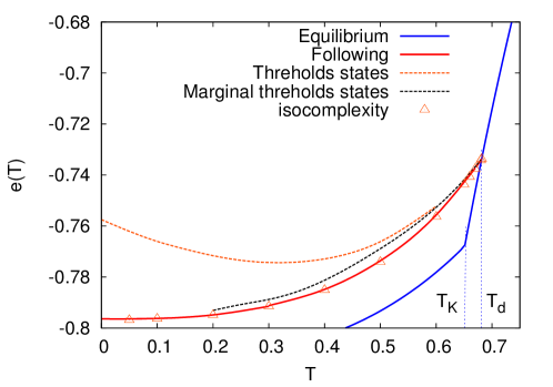
Let us remind the different type of predictions for behavior of slow annealing; they are summarized in Fig.1.

For a long time, the dominating idea has been that one simply has to compute the so called ”thresholds states”. There high energy energy minima in the energy landscape. The idea of such computation is count how many minima they are at a given energy, and to compute for which energy they are most numerous. This, according to this idea, allows to locate at which energy there are minima that can, most likely, trap the dynamics. The corresponding energy is depicted as “thresholds states” in Fig. 1. This idea is popular, mostly because it works perfectly in the simple spherical $p$-spin model[1, 2, 3, 4], however, as discussed for instance in [25], the situations is much more complicated already in the mixed spherical $p$-spin glass model.

It was soon realized [26, 16] that in fact most of these states are actually the result of a computation that is not self-consistent (unstable towards more steps of repica symmetry breaking), and that the threshold states of “stable” (or at least marginally stable) states is much lower. Computing correctly those turned out to be a complicate task that has been finally achieved by Rizzo in [27]. The result is shown in Fig. 1 as “marginal states”. To be precise, we refer as threshold states the (unstable) 1RSB ones, and to the marginal states the (marginal) full RSB ones [27].

However, as discussed in e.g. [10, 11, 26, 12, 16, 6, 7], it may be a bit naive to assume that a Monte-Carlo annealing will just end up in the most numerous states, and that was the motivation for the idea for following states that started at $T_{d}$. This is why iso-complexity was introduced: It is proposed to count the number of equilibrium states at $T_{d}$, and then to consider the energies at $T<T_{d}$ for which the number of states is equal to the one at $T_{d}$. Iso-complexity leads indeed to a lower bound on adiabatic annealings, because in order to end up at lower energies one would have to be exponentially lucky. Indeed, if one is trap in one of $e^{N\Sigma_{1}}$ similar states at an energy $e_{1}$, and if the total number of states at $e_{2}<e_{1}$ is $e^{N\Sigma_{2}}$, with $Sigma_{2}<Sigma_{1}$, it is exponentially unlikly that any of these correponds to the one at $e_{1}$.

In fact, the iso-complexity is only an approximation of the following state formalism (where we explicitly follow states), and explicit differences can be seen (see for instance [6, 7]) however, since the following state computation itself can be rather involved (see [13]) and in some cases (for low enough temperature) we could only do an approximated computation (see [6, 7, 25]). As shown in Fig. 1, however, the results of the two approach is extremely close in the 3-spin model (see also [6, 7] for the diluted case), at least in the case when one starts from $T=T_{d}$ (actually, there are more devitaion for the the states starting from $T<T_{d}$, as seen in [6, 7]). The question is now how these rather different predictions compare with simulations.

4 Annealings follow the following state computation

Figure 2: Annealings starting from an equilibrated configuration at high temperature $T_{1}>T_{d}=0.6825$ in the 3-spin glass problem for $N=50000$. Left: The energy of annealings from $T_{1}=0.7$ with different cooling rates is shown together with the equilibrium solution of the model (in blue) and the following state prediction (in red). Right: As in the left figure, but with different starting points. For comparison, we also shows the energy of the thresholds states (dashed orange line) and the marginal thresholds states (dashed black line). Annealings have no problems going below these energies that do not seem to affect its behavior.

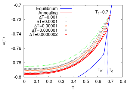
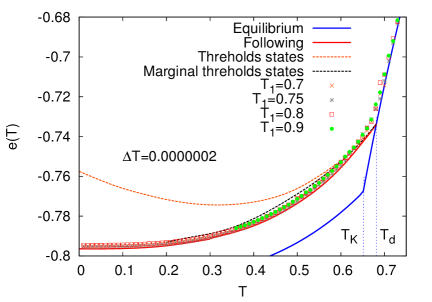
The results of annealings starting from an equilibrated configuration at $T_{1}>T_{d}$ are shown in Fig.2 for different rates. They are clearly approaching the following state predictions as the rate decreases $\Delta T\to 0$. We also show these annealing using only the smallest rate (and demonstrate that the starting temperature does not matter as long as it is larger than $T_{d}$). It is striking how easily the Monte-Carlo dynamics is able to go beyond the thresholds state, marginal or not.

These data clearly demonstrate that annealings are not at all sensitive to the thresholds states, and that the following states of isocomplexity consideration are the correct ones in this case. It is also striking how these two are similar (although definitely not equal). For models with a discontinuous first order transition, it thus seem that iso-complexity is a very acceptable approximation. It would be interesting to see how generic this is (see [6, 7]. for discussion in the XORSAT model, [25] for the spherical model, and the reviez [28] for hard sphere.).

Figure 3: Annealings starting from an equilibrated configuration at low temperature $T_{1}\leq T_{d}$ in the $3$-spin glass problem for $N=50000$. Left: The energy of annealings from three different starting temperatures $T_{1}=T_{d},0.67,0.66$ with slow cooling rate is shown together with the equilibrium solution of the model (in blue) and the following state prediction (in red), demonstrating a perfect agreement. Right: overlap with the starting configuration at $T_{1}=0.67,0.66$ as a function of the temperature. The approximated nature of the analytical solution (in full line) appears here as it predicts a non monotonous behavior that is not seen in the Monte-Carlo simulation. Indeed, the following state computation is unstable towards more complicated symmetry breaking for $T<0.55$ ($T_{1}=0.67$) and for $T<0.49$ ($T_{1}=0.66$).

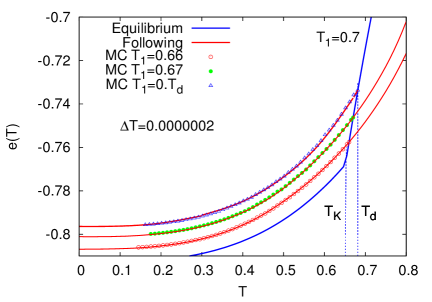
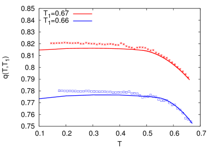
This can also be clearly seen from annealing from temperature below $T_{d}$ (see Fig. 3) where the agreement is again perfect with the following state computations. Still, the approximative nature of the computation should be clear from deviation in the overlap (left figure) which display non physical behavior in the following state computation. The point is that this computation is done in a 1RSB formalism, in a region where a more complicated ansatz should be used (see also [25]). In fact, when the state is unstable, one should in principle performs a more involved computation and follows the pseudo-dynamics idea of[12, 13]. This is, however, more complicated, and we shall not attempt to discuss these points here.

5 What about quenches?

Finally, we also performed direct quenches from a high temperature to a small one. The situation here is more complicated as there is no theory equivalent to the following state computation yet (but see [13]).

Figure 4: Quenches starting from equilibrated configuration at temperature $T_{1}>T_{d}$ to $T_{2}<T_{d}$ for $N=20000$. Left: quenches to $T_{2}=0.6$ and $T_{2}=0.5$, Right:quenches to $T_{2}=0.4$ and $T_{2}=0.3$. Although an extrapolation is difficult, it seems —especially in the right figure— that the asymptotic energies are larger than the marginal threshold states prediction. However, perhaps surprisingly, they are close to the standard unstable threshold states, as also noticed in [16].

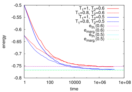
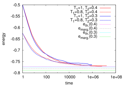
However, the simulation seems to indicate that the quenches converge to higher energies than the annealing. In fact, they are surprisingly close to the thresholds state (but, again surprisingly, higher from the marginal ones). Although it is difficult to draw firm conclusion from these data, the role of the marginal thresholds in the dynamics is not apparent. Also, it is not clear that the starting temperature is relevant, which also seem contradictory to the idea that quenches are different to annealing in the long runs. The most recent idea, proposed by Rizzo [27], proposed that (up to logarithmic corrections) quenches will tend to a new threshold energy. This is a promising idea that await a numerical confirmation. Surprisingly (given the long lasting interest in spin glasses) we are aware of very few simulations of this problem, and a deep, systematic investigation, would be welcome.

6 Conclusion and perspective

The conclusion of this short proceeding are two folds: 1) we wanted to illustrate how good the prediction of the following state are (and how good the isocomplexity approximation can be in some case) and 2) nothing seems to happens at energies connected to thresholds or marginal threshold states. We hope that this presentation of the data will convince the community that the bridge between statics and dynamics is not going through thresholds states consideration, but rather through following states considerations.

For quenches, instead, the situations is unclear and more work on the subject is welcome, in particular to test the proposition of [27].

We hope that this short presentation will help to clarify the situation and will help to motivate further works in this direction, perhaps following the idea of pseudo-dynamics[12, 13].

References

- [1] Cugliandolo L F and Dean D S 1995 J. Phys. A 28 4213
- [2] Cugliandolo L F and Kurchan J 1993 Phys. Rev. Lett. 71 173
- [3] Bouchaud J P and Dean D 1995 J. Phys. I, France 5 265–286
- [4] Bouchaud J P, Cugliandolo L, Kurchan J and Mézard M 1998 Spin Glasses and Random Fields ed Young A P (Singapore: World Scientific)
- [5] Kirkpatrick S, Gelatt, Jr C D and Vecchi M P 1983 Science 220 671
- [6] Krzakala F and Zdeborová L 2010 EPL (Europhysics Letters) 90 66002
- [7] Zdeborová L and Krzakala F 2010 Physical Review B 81 224205
- [8] Gross D and Mézard M 1984 Nucl. Phys. B 240 431
- [9] Franz S and Parisi G 1997 Phys. Rev. Lett. 79 2486–2489
- [10] Barrat A, Franz S and Parisi G 1997 J. Phys. A 30 5593–5612
- [11] Franz S and Parisi G 1998 Physica A 261 317–339
- [12] Krzakala F and Kurchan J 2007 Phys. Rev. E 76 021122
- [13] Franz S, Parisi G and Urbani P 2012 arXiv preprint arXiv:1212.4291
- [14] T R Kirkpatrick D T and Wolynes P G 1989 Phys. Rev. A 40 1045
- [15] Bouchaud J P and Biroli G 2004 J. Chem. Phys. 121 7347
- [16] Montanari A and Ricci-Tersenghi F 2004 Phys. Rev. B 70 134406
- [17] Kirkpatrick T R and Thirumalai D 1989 J. Phys. A 22 L149
- [18] Ozeki Y 1997 Journal of Physics: Condensed Matter 9 11171
- [19] Montanari A and Semerjian G 2006 J. Stat. Phys. 124 103–189
- [20] Achlioptas D and Coja-Oghlan A 2008 Foundations of Computer Science, 2008. FOCS ’08. IEEE 49th Annual IEEE Symposium on pp 793–802 ISSN 0272-5428
- [21] Krzakala F and Zdeborová L 2009 Phys. Rev. Lett. 102 238701
- [22] Krzakala F and Zdeborová L 2011 The Journal of Chemical Physics 134 034512
- [23] Krzakala F and Zdeborová L 2011 The Journal of Chemical Physics 134 034513
- [24] Zdeborová L and Krzakala F 2011 SIAM J. Discrete Math. 25 750–770
- [25] Sun Y, Crisanti A, Krzakala F, Leuzzi L and Zdeborová L 2012 J. Stat. Mech. 2012 P07002
- [26] Montanari A and Ricci-Tersenghi F 2003 Eur. Phys. J. B 33 339–346
- [27] Rizzo T 2013 arXiv preprint arXiv:1305.2070
- [28] Parisi G and Zamponi F 2010 Rev. Mod. Phys. 82(1) 789–845