Bs,d0μμ¯superscriptsubscript𝐵𝑠𝑑0𝜇¯𝜇B_{s,d}^{0}\to\mu\bar{\mu} and BXsγ𝐵subscript𝑋𝑠𝛾B\to X_{s}\gamma in the R𝑅R-parity violating MSSM

H. K. Dreiner dreiner@uni-bonn.de    K. Nickel nickel@th.physik.uni-bonn.de    F. Staub fnstaub@physik.uni-bonn.de Bethe Center for Theoretical Physics & Physikalisches Institut der Universität Bonn,
Nußallee 12, 53115 Bonn, Germany
Abstract

The recent measurements of Bs0μμ¯subscriptsuperscript𝐵0𝑠𝜇¯𝜇B^{0}_{s}\to\mu\bar{\mu} decay candidates at the LHC consistent with the standard model rate, and the improving upper limits for Bd0μμ¯subscriptsuperscript𝐵0𝑑𝜇¯𝜇B^{0}_{d}\to\mu\bar{\mu}\, can strongly constrain beyond the standard model physics. For example, in supersymmetric models with broken R𝑅R-parity (RpV), they restrict the size of the new couplings. We use the combination of the public software packages SARAH and SPheno to derive new bounds on several combinations of RpV𝑅pVR\mathrm{pV} couplings. We improve existing limits for the couplings which open tree-level decay channels and state new limits for combinations which induce loop contributions. This is the first study which performs a full one-loop analysis of these observables in the context of R𝑅R-parity violation. It turns out that at one-loop despite the strong experimental limits only combinations of R𝑅R-parity violating couplings are constrained which include third generation fermions. We compare our limits with those obtained via BXsγ𝐵subscript𝑋𝑠𝛾B\to X_{s}\gamma and discuss the differences.

preprint: BONN-TH-2013-14

I Introduction

The first experimentation phase of the experiments at the Large Hadron Collider (LHC) is completed. However, there is no evidence or hint up to now for superpartner particles as predicted by the well-motivated theory of supersymmetry (SUSY) or any other physics beyond the Standard Model (SM) :2012rz ; Chatrchyan:2012jx ; CMS-PAS-SUS-11-022 ; CMS-PAS-SUS-12-005 ; :2012mfa . The simplest SUSY scenarios like the constrained minimal supersymmetric standard model (CMSSM) is under pressure by the ongoing non-discovery, leading to the exclusion of large areas of parameter space Bechtle:2012zk ; Ghosh:2012dh ; Buchmueller:2012hv . In addition, the observed mass of mh126GeVsubscript𝑚126GeVm_{h}\approx 126~{}{\text{Ge}\text{V}} for the Higgs boson Atlas:2012gk ; CMS:2012gu is rather hard to realize in the CMSSM and requires heavy SUSY spectra to push the predicted Higgs mass to that level pMSSM ; Bechtle:2012zk ; Buchmueller:2012hv . However, this applies only if the stop and the other sfermion masses are related. While heavy stops with a large mass splitting are needed to explain the Higgs mass, the other sfermion contributions are usually sub-dominant in this context. Hence, these states could in principle be much lighter. However they are constrained by direct searches. Therefore SUSY models with different signatures like R𝑅R-parity violation (RpV) are more interesting since they can significantly soften the mass limits Hall:1983id ; rpv ; Barbier:2004ez ; rpvsearches ; Franceschini:2012za ; Evans:2012bf and provide a rich collider phenomenology Dreiner:2012wm . On the other hand, beyond the standard model (BSM) physics can not only manifest itself directly at collider searches, but also indirectly via quantum corrections to (rare) standard model processes. Interesting processes are those which rarely occur in the SM but which can be measured with high accuracy. In this context quark flavor changing neutral currents (qFCNC), like BXsγ𝐵subscript𝑋𝑠𝛾B\to X_{s}\gamma Barbieri:1993av ; bsgamma1 ; bsgamma2 ; BsGamma and the decays of the neutral B0superscript𝐵0B^{0} mesons (Bs0,Bd0superscriptsubscript𝐵𝑠0superscriptsubscript𝐵𝑑0B_{s}^{0},B_{d}^{0}) into a pair of leptons bsmumu-susy are interesting candidates to look for deviations from the SM.

In this paper we focus on the constraints on R𝑅R-parity violating couplings derived from the experimental limits on Bs,d0μμ¯subscriptsuperscript𝐵0𝑠𝑑𝜇¯𝜇B^{0}_{s,d}\to\mu\bar{\mu} and BXsγ𝐵subscript𝑋𝑠𝛾B\to X_{s}\gamma. Previous studies of BXsγ𝐵subscript𝑋𝑠𝛾B\to X_{s}\gamma in this context assumed a SUSY spectra no longer in agreement with experimental data deCarlos:1996yh ; Kong:2004cp , while for B𝐵B-meson decays to two leptons only the new tree level contributions have been studied so far Dreiner:2006gu ; Li:2013fa ; Yeghiyan:2013upa . We perform a full one-loop analysis of Bs,d0μμ¯subscriptsuperscript𝐵0𝑠𝑑𝜇¯𝜇B^{0}_{s,d}\to\mu\bar{\mu} which allows us to constrain new combinations of couplings besides those at tree level. For this purpose we use the combination of public software packages SARAH sarah and SPheno spheno . SARAH creates new source code for SPheno which can be used for the numerical study of a given model. Recently, this functionality has been extended to provide a full one-loop calculation of Bs,d0¯subscriptsuperscript𝐵0𝑠𝑑¯B^{0}_{s,d}\to\ell\bar{\ell} Dreiner:2012dh . We compare the new limits with those obtained by a revised study of BXsγ𝐵subscript𝑋𝑠𝛾B\to X_{s}\gamma and discuss the differences between both observables.

We briefly review the main basics of the B𝐵B-decays in sec. II and introduce the MSSM with R𝑅R-parity violation in sec. III. We explain the numerical setup in sec. IV and present our results in sec. V, before concluding in sec. VI.

II Standard model predictions and measurements for Bs,d0μμ¯superscriptsubscript𝐵𝑠𝑑0𝜇¯𝜇B_{s,d}^{0}\to\mu\bar{\mu} and BXsγ𝐵subscript𝑋𝑠𝛾B\to X_{s}\gamma

II.1 Bs,d0μμ¯superscriptsubscript𝐵𝑠𝑑0𝜇¯𝜇B_{s,d}^{0}\to\mu\bar{\mu}

The semi-leptonic B0superscript𝐵0B^{0} decay is described by a matrix element \mathcal{M} as a function of the form factors FS,FP,FV,FAsubscript𝐹𝑆subscript𝐹𝑃subscript𝐹𝑉subscript𝐹𝐴F_{S},F_{P},F_{V},F_{A} for the scalar, pseudoscalar, vector and axial vector currents. The squared matrix element Dedes:2008iw of Bq0k¯lsuperscriptsubscript𝐵𝑞0subscript𝑘subscript¯𝑙B_{q}^{0}\to\ell_{k}\bar{\ell}_{l},

(4π)4||2superscript4𝜋4superscript2\displaystyle(4\pi)^{4}\left|{\mathcal{M}}\right|^{2} =2|FS|2[MBq02(ml+mk)2]+2|FP|2[MBq02(mlmk)2]absent2superscriptsubscript𝐹𝑆2delimited-[]superscriptsubscript𝑀subscriptsuperscript𝐵0𝑞2superscriptsubscript𝑚𝑙subscript𝑚𝑘22superscriptsubscript𝐹𝑃2delimited-[]superscriptsubscript𝑀subscriptsuperscript𝐵0𝑞2superscriptsubscript𝑚𝑙subscript𝑚𝑘2\displaystyle=2\left|{F_{S}}\right|^{2}\left[M_{B^{0}_{q}}^{2}-(m_{l}+m_{k})^{2}\right]+2\left|{F_{P}}\right|^{2}\left[M_{B^{0}_{q}}^{2}-(m_{l}-m_{k})^{2}\right] (1)
+2|FV|2[MBq02(mkml)2(mk2ml2)2]2superscriptsubscript𝐹𝑉2delimited-[]superscriptsubscript𝑀subscriptsuperscript𝐵0𝑞2superscriptsubscript𝑚𝑘subscript𝑚𝑙2superscriptsuperscriptsubscript𝑚𝑘2superscriptsubscript𝑚𝑙22\displaystyle+2\left|{F_{V}}\right|^{2}\left[M_{B^{0}_{q}}^{2}(m_{k}-m_{l})^{2}-(m_{k}^{2}-m_{l}^{2})^{2}\right]
+2|FA|2[MBq02(mk+ml)2(mk2ml2)2]2superscriptsubscript𝐹𝐴2delimited-[]superscriptsubscript𝑀subscriptsuperscript𝐵0𝑞2superscriptsubscript𝑚𝑘subscript𝑚𝑙2superscriptsuperscriptsubscript𝑚𝑘2superscriptsubscript𝑚𝑙22\displaystyle+2\left|{F_{A}}\right|^{2}\left[M_{B^{0}_{q}}^{2}(m_{k}+m_{l})^{2}-(m_{k}^{2}-m_{l}^{2})^{2}\right]
+4(FsFV)(mlmk)[MBq02+(mk+ml)2]4subscript𝐹𝑠superscriptsubscript𝐹𝑉subscript𝑚𝑙subscript𝑚𝑘delimited-[]superscriptsubscript𝑀subscriptsuperscript𝐵0𝑞2superscriptsubscript𝑚𝑘subscript𝑚𝑙2\displaystyle+4\Re(F_{s}F_{V}^{*})(m_{l}-m_{k})\left[M_{B^{0}_{q}}^{2}+(m_{k}+m_{l})^{2}\right]
+4(FPFA)(ml+mk)[MBq02(mkml)2],4subscript𝐹𝑃superscriptsubscript𝐹𝐴subscript𝑚𝑙subscript𝑚𝑘delimited-[]superscriptsubscript𝑀subscriptsuperscript𝐵0𝑞2superscriptsubscript𝑚𝑘subscript𝑚𝑙2\displaystyle+4\Re(F_{P}F_{A}^{*})(m_{l}+m_{k})\left[M_{B^{0}_{q}}^{2}-(m_{k}-m_{l})^{2}\right]\,,

determines the branching ratio BR(Bq0k¯l)BRsuperscriptsubscript𝐵𝑞0subscript𝑘subscript¯𝑙\text{BR}\,(B_{q}^{0}\to\ell_{k}\bar{\ell}_{l}) Dedes:2008iw ,

BR(Bq0k¯l)=τBq016π||2MBq01(mk+mlMBq0)21(mkmlMBq0)2,BRsuperscriptsubscript𝐵𝑞0subscript𝑘subscript¯𝑙subscript𝜏subscriptsuperscript𝐵0𝑞16𝜋superscript2subscript𝑀superscriptsubscript𝐵𝑞01superscriptsubscript𝑚𝑘subscript𝑚𝑙subscript𝑀superscriptsubscript𝐵𝑞021superscriptsubscript𝑚𝑘subscript𝑚𝑙subscript𝑀superscriptsubscript𝐵𝑞02\text{BR}\,(B_{q}^{0}\to\ell_{k}\bar{\ell}_{l})=\frac{\tau_{B^{0}_{q}}}{16\pi}\frac{\left|{\mathcal{M}}\right|^{2}}{M_{B_{q}^{0}}}\sqrt{1-\left(\frac{m_{k}+m_{l}}{M_{B_{q}^{0}}}\right)^{2}}\sqrt{1-\left(\frac{m_{k}-m_{l}}{M_{B_{q}^{0}}}\right)^{2}}, (2)

where τBq0subscript𝜏subscriptsuperscript𝐵0𝑞\tau_{B^{0}_{q}} is the lifetime of the mesons and mksubscript𝑚𝑘m_{k} the mass of the lepton ksubscript𝑘\ell_{k}. Note that the form factor FVsubscript𝐹𝑉F_{V} does not contribute to Eq. (1) in the case l=k𝑙𝑘l=k. These decays are fixed in the SM by the CKM matrix and the form factors can be calculated with a high precision. The predicted branching ratios for Bs,d0μμ¯subscriptsuperscript𝐵0𝑠𝑑𝜇¯𝜇B^{0}_{s,d}\to\mu\bar{\mu} are Buras:2012ru .

BR(Bs0μμ¯)SMBRsubscriptsubscriptsuperscript𝐵0𝑠𝜇¯𝜇SM\displaystyle\text{BR}(B^{0}_{s}\to\mu\bar{\mu})\,_{\text{SM}} =\displaystyle= (3.23±0.27)109,plus-or-minus3.230.27superscript109\displaystyle(3.23\pm 0.27)\cdot 10^{-9}, (3)
BR(Bd0μμ¯)SMBRsubscriptsubscriptsuperscript𝐵0𝑑𝜇¯𝜇SM\displaystyle\text{BR}(B^{0}_{d}\to\mu\bar{\mu})\,_{\text{SM}} =\displaystyle= (1.07±0.10)1010.plus-or-minus1.070.10superscript1010\displaystyle(1.07\pm 0.10)\cdot 10^{-10}. (4)

The errors include experimental uncertainties of the involved parameters as well as uncertainties from higher orders and scheme dependence. These predictions neglect the CP violation in the Bssubscript𝐵𝑠B_{s}B¯ssubscript¯𝐵𝑠\bar{B}_{s} system which leads to a difference in the decay widths for Bs0subscriptsuperscript𝐵0𝑠B^{0}_{s} and B¯s0subscriptsuperscript¯𝐵0𝑠\bar{B}^{0}_{s} Raven:2012fb . When it is not known in the experiment whether a pair of muons comes from the decay of a Bs0superscriptsubscript𝐵𝑠0B_{s}^{0} or a B¯s0superscriptsubscript¯𝐵𝑠0\bar{B}_{s}^{0}, the untagged decay rate is measured. Therefore, one has to compare the LHC limits with the averaged branching ratio of Bs0μμ¯subscriptsuperscript𝐵0𝑠𝜇¯𝜇B^{0}_{s}\to\mu\bar{\mu} and B¯s0μμ¯subscriptsuperscript¯𝐵0𝑠𝜇¯𝜇\bar{B}^{0}_{s}\to\mu\bar{\mu} Buras:2013uqa

BR¯(Bs0μμ¯)SM¯BRsubscriptsuperscriptsubscript𝐵𝑠0𝜇¯𝜇SM\displaystyle\overline{\text{BR}\,}({B_{s}^{0}\to\mu\bar{\mu}})_{\text{SM}} =(3.56±0.18)109absentplus-or-minus3.560.18superscript109\displaystyle=(3.56\pm 0.18)\cdot 10^{-9} (5)

The width difference between Bd0superscriptsubscript𝐵𝑑0B_{d}^{0} and B¯d0superscriptsubscript¯𝐵𝑑0\bar{B}_{d}^{0} is much smaller than for the Bssubscript𝐵𝑠B_{s} system and is not measured accurately. Hence, we use the untagged rate in the following. Eq. (5) is consistent with the recently updated measurements for Bsμμ¯subscript𝐵𝑠𝜇¯𝜇B_{s}\to\mu\bar{\mu} at the LHC LHCb:2012ct ; LHCb:2013 ,

BR(Bs0μμ¯)BRsubscriptsuperscript𝐵0𝑠𝜇¯𝜇\displaystyle\text{BR}(B^{0}_{s}\to\mu\bar{\mu})\, =(2.91.0+1.1)×109,absentsubscriptsuperscript2.91.11.0superscript109\displaystyle=(2.9^{+1.1}_{-1.0})\times 10^{-9}, (6)

In addition, the experimental upper limit for LHCb:2013

BR(Bd0μμ¯)BRsubscriptsuperscript𝐵0𝑑𝜇¯𝜇\displaystyle\text{BR}(B^{0}_{d}\to\mu\bar{\mu})\, <7.4×10¹⁰,absent7.4superscript1010\displaystyle<7.4\times 10^{-10}, (7)

is approaching the SM expectation. These measurements shrink the space where one can hope to see new physics. Especially SUSY scenarios with large tanβ𝛽\tan\beta can lead to a prediction of these decays which is now ruled out Haisch:2012re .

To compare the bounds of these two observables with our calculation and to put limits on the SUSY contributions, we consider the ratio

Risubscript𝑅𝑖\displaystyle R_{i} BR(Bi0μμ¯)SUSYBR(Bi0μμ¯)SM,(i=s,d),absentBRsubscriptsuperscriptsubscript𝐵𝑖0𝜇¯𝜇SUSYBRsubscriptsuperscriptsubscript𝐵𝑖0𝜇¯𝜇SM𝑖𝑠𝑑\displaystyle\equiv\frac{\text{BR}(B_{i}^{0}\to\mu\bar{\mu})\,_{\text{SUSY}}}{\text{BR}(B_{i}^{0}\to\mu\bar{\mu})\,_{\text{SM}}},\quad(i=s,d), (8)

in which the finite width effects factor out. Note, BRSUSYsubscriptBRSUSY\text{BR}_{\text{SUSY}} includes also the SM contributions. Together with Eqs. (6) and (7), we obtain an allowed range of

0.43<Rs<1.35,0.43subscript𝑅𝑠1.35\displaystyle 0.43<R_{s}<1.35\,, (9)
Rd<8.30.subscript𝑅𝑑8.30\displaystyle R_{d}<8.30\,. (10)

Here, we assumed a combined total uncertainty of 20% on the upper (and lower) limit, which includes the errors of the SM prediction and of our SUSY calculation.

II.2 BXsγ𝐵subscript𝑋𝑠𝛾B\to X_{s}\gamma

The main contribution to the radiative B-meson decay B¯Xsγ¯𝐵subscript𝑋𝑠𝛾\bar{B}\rightarrow X_{s}\gamma stems from the partonic process bsγ𝑏𝑠𝛾b\rightarrow s\gamma. The standard model prediction bsgamma1 ; bsgamma2 ; BsGamma

Br(BXsγ)SM=(3.15±0.23)×104,Brsubscript𝐵subscript𝑋𝑠𝛾𝑆𝑀plus-or-minus3.150.23superscript104\text{Br}(B\to X_{s}\gamma)_{SM}=(3.15\pm 0.23)\times 10^{-4}, (11)

has to be compared with the experimental limit of Beringer:1900zz

Br(BXsγ)=(3.55±0.24±0.09)×104.Br𝐵subscript𝑋𝑠𝛾plus-or-minus3.550.240.09superscript104\text{Br}(B\to X_{s}\gamma)=(3.55\pm 0.24\pm 0.09)\times 10^{-4}\,. (12)

To derive bounds on the RpV𝑅pVR\mathrm{pV} couplings from BXsγ𝐵subscript𝑋𝑠𝛾B\to X_{s}\gamma we follow closely the approach of Ref. Haisch:2012re and use as 95% C.L. limit

0.89<RXsγ<1.33,0.89subscript𝑅subscript𝑋𝑠𝛾1.330.89<R_{X_{s}\gamma}<1.33\,, (13)

with

RXsγBR(BXsγ)SUSYBR(BXsγ)SM.subscript𝑅subscript𝑋𝑠𝛾BRsubscript𝐵subscript𝑋𝑠𝛾𝑆𝑈𝑆𝑌BRsubscript𝐵subscript𝑋𝑠𝛾𝑆𝑀R_{X_{s}\gamma}\equiv\frac{\text{BR}(B\to X_{s}\gamma)\,_{SUSY}}{\text{BR}(B\to X_{s}\gamma)\,_{SM}}. (14)

III R𝑅R-parity violation and neutral B-meson decays

R𝑅R-parity is a discrete Z2subscript𝑍2Z_{2} symmetry of the MSSM which is defined as

RP=(1)3(BL)+2s,subscript𝑅𝑃superscript13𝐵𝐿2𝑠R_{P}=(-1)^{3(B-L)+2s}\,, (15)

where s𝑠s is the spin of the field and B𝐵B, L𝐿L are its baryon respectively lepton number. If we just allow for R𝑅R-parity conserving parameters and assume the minimal set of superfields which is anomaly free and needed to reproduce the SM, we are left with the (renormalizable) superpotential of the MSSM

WR=Yeab𝐋a𝐄¯b𝐇d+Ydab𝐐a𝐃¯b𝐇d+Yuab𝐐a𝐔¯b𝐇u+μ𝐇u𝐇d.subscript𝑊𝑅subscriptsuperscript𝑌𝑎𝑏𝑒subscript𝐋𝑎subscript¯𝐄𝑏subscript𝐇𝑑subscriptsuperscript𝑌𝑎𝑏𝑑subscript𝐐𝑎subscript¯𝐃𝑏subscript𝐇𝑑subscriptsuperscript𝑌𝑎𝑏𝑢subscript𝐐𝑎subscript¯𝐔𝑏subscript𝐇𝑢𝜇subscript𝐇𝑢subscript𝐇𝑑W_{R}=Y^{ab}_{e}\,{\bf L}_{a}{\bf{\bar{E}}}_{b}{\bf H}_{d}+Y^{ab}_{d}\,{\bf Q}_{a}{\bf{\bar{D}}}_{b}{\bf H}_{d}+Y^{ab}_{u}{\bf Q}_{a}{\bf{\bar{U}}}_{b}{\bf H}_{u}+\mu\,{\bf H}_{u}{\bf H}_{d}\,. (16)

Here a,b=1,2,3formulae-sequence𝑎𝑏123a,b=1,2,3 are generation indices, while we suppressed color and isospin indices. The corresponding standard soft-breaking terms for the scalar fields L~,E~,Q~,U~,D~,Hd,Hu~𝐿~𝐸~𝑄~𝑈~𝐷subscript𝐻𝑑subscript𝐻𝑢\widetilde{L},\widetilde{E},\widetilde{Q},\widetilde{U},\widetilde{D},H_{d},H_{u} and the gauginos B~,W~,g~~𝐵~𝑊~𝑔\widetilde{B},\widetilde{W},\widetilde{g} read

SB,RsubscriptSB𝑅\displaystyle-\mathscr{L}_{\text{SB},R} =\displaystyle= mHu2|Hu|2+mHd2|Hd|2+Q~mq~2Q~+L~ml~2L~+D~md~2D~+U~mu~2U~+E~me~2E~superscriptsubscript𝑚subscript𝐻𝑢2superscriptsubscript𝐻𝑢2superscriptsubscript𝑚subscript𝐻𝑑2superscriptsubscript𝐻𝑑2superscript~𝑄superscriptsubscript𝑚~𝑞2~𝑄superscript~𝐿superscriptsubscript𝑚~𝑙2~𝐿superscript~𝐷superscriptsubscript𝑚~𝑑2~𝐷superscript~𝑈superscriptsubscript𝑚~𝑢2~𝑈superscript~𝐸superscriptsubscript𝑚~𝑒2~𝐸\displaystyle m_{H_{u}}^{2}|H_{u}|^{2}+m_{H_{d}}^{2}|H_{d}|^{2}+\widetilde{Q}^{\dagger}m_{\widetilde{q}}^{2}\widetilde{Q}+\widetilde{L}^{\dagger}m_{\widetilde{l}}^{2}\widetilde{L}+\widetilde{D}^{\dagger}m_{\widetilde{d}}^{2}\widetilde{D}+\widetilde{U}^{\dagger}m_{\widetilde{u}}^{2}\widetilde{U}+\widetilde{E}^{\dagger}m_{\widetilde{e}}^{2}\widetilde{E} (17)
+12(M1B~B~+M2W~iW~i+M3g~αg~α+h.c.)\displaystyle+\frac{1}{2}\left(M_{1}\,\widetilde{B}\widetilde{B}+M_{2}\,\widetilde{W}_{i}\widetilde{W}^{i}+M_{3}\,\widetilde{g}_{\alpha}\widetilde{g}^{\alpha}+h.c.\right)
+(Q~TuU~Hu+Q~TdD~Hd+L~TeE~Hd+BμHuHd+h.c.).~𝑄subscript𝑇𝑢superscript~𝑈subscript𝐻𝑢~𝑄subscript𝑇𝑑superscript~𝐷subscript𝐻𝑑~𝐿subscript𝑇𝑒superscript~𝐸subscript𝐻𝑑subscript𝐵𝜇subscript𝐻𝑢subscript𝐻𝑑h.c.\displaystyle+(\widetilde{Q}T_{u}\widetilde{U}^{\dagger}H_{u}+\widetilde{Q}T_{d}\widetilde{D}^{\dagger}H_{d}+\widetilde{L}T_{e}\widetilde{E}^{\dagger}H_{d}+B_{\mu}H_{u}H_{d}+\text{h.c.})\thickspace.

However, there are additional renormalizable interactions which are allowed by gauge invariance in the superpotential but break R𝑅R-parity:

Wtrisubscript𝑊triitalic-L̸\displaystyle W_{\text{tri}\not{L}} =12λijk𝐋i𝐋j𝐄¯k+λijk𝐋i𝐐j𝐃¯k,absent12subscript𝜆𝑖𝑗𝑘subscript𝐋𝑖subscript𝐋𝑗subscript¯𝐄𝑘superscriptsubscript𝜆𝑖𝑗𝑘subscript𝐋𝑖subscript𝐐𝑗subscript¯𝐃𝑘\displaystyle=\frac{1}{2}\lambda_{ijk}\cdot{\bf L}_{i}{\bf L}_{j}{\bf{\bar{E}}}_{k}+\lambda_{ijk}^{\prime}\cdot{\bf L}_{i}{\bf Q}_{j}{\bf{\bar{D}}}_{k}, (18)
Wbisubscript𝑊biitalic-L̸\displaystyle W_{\text{bi}\not{L}} =κi𝐋i𝐇u,absentsubscript𝜅𝑖subscript𝐋𝑖subscript𝐇𝑢\displaystyle=\kappa_{i}{\bf L}_{i}{\bf H}_{u}, (19)
Wsubscript𝑊italic-B̸\displaystyle W_{\not{B}} =12λijk′′𝐔¯i𝐃¯j𝐃¯k.absent12superscriptsubscript𝜆𝑖𝑗𝑘′′subscript¯𝐔𝑖subscript¯𝐃𝑗subscript¯𝐃𝑘\displaystyle=\frac{1}{2}\lambda_{ijk}^{\prime\prime}{\bf{\bar{U}}}_{i}{\bf{\bar{D}}}_{j}{\bf{\bar{D}}}_{k}. (20)

The bi- and trilinear operators in eqs. (18) and (19) violate lepton number, the operators in eq. (20) violate baryon number. The corresponding soft-breaking terms for these interactions are

trisubscripttriitalic-L̸\displaystyle-\mathscr{L}_{\text{tri}\not{L}} =12TλijkL~iL~jE~k+TλijkL~iQ~jD~k+h.c.,absent12subscript𝑇subscript𝜆𝑖𝑗𝑘subscript~𝐿𝑖subscript~𝐿𝑗subscript~𝐸𝑘subscript𝑇superscriptsubscript𝜆𝑖𝑗𝑘subscript~𝐿𝑖subscript~𝑄𝑗subscript~𝐷𝑘h.c.\displaystyle=\frac{1}{2}T_{\lambda_{ijk}}\cdot\widetilde{L}_{i}\widetilde{L}_{j}\widetilde{E}_{k}+T_{\lambda_{ijk}^{\prime}}\cdot\widetilde{L}_{i}\widetilde{Q}_{j}\widetilde{D}_{k}+\text{h.c.}\,, (21)
bisubscriptbiitalic-L̸\displaystyle-\mathscr{L}_{\text{bi}\not{L}} =BκiL~iHu+h.c.,absentsubscript𝐵subscript𝜅𝑖subscript~𝐿𝑖subscript𝐻𝑢h.c.\displaystyle=B_{\kappa_{i}}\widetilde{L}_{i}H_{u}+\text{h.c.}\,, (22)
subscriptitalic-B̸\displaystyle-\mathscr{L}_{\not{B}} =12Tλijk′′U~iαD~jβD~kγϵαβγ+h.c..absent12superscriptsubscript𝑇subscript𝜆𝑖𝑗𝑘′′superscriptsubscript~𝑈𝑖𝛼superscriptsubscript~𝐷𝑗𝛽superscriptsubscript~𝐷𝑘𝛾subscriptitalic-ϵ𝛼𝛽𝛾h.c.\displaystyle=\frac{1}{2}T_{\lambda_{ijk}}^{\prime\prime}\widetilde{U}_{i}^{\alpha}\widetilde{D}_{j}^{\beta}\widetilde{D}_{k}^{\gamma}\epsilon_{\alpha\beta\gamma}+\text{h.c.}\,. (23)

The terms involving λ𝜆\lambda (or λ,λ′′superscript𝜆superscript𝜆′′\lambda^{\prime},\lambda^{{\prime\prime}}) are called LLE interactions (or LQD, UDD) in the following. Since proton decay is always triggered by a combination of baryon and lepton number violating couplings, a model with either italic-L̸\not{L} or italic-B̸\not{B} terms is safe from rapid proton decay. We are going to study in the following the impact of the new couplings present in Wtrisubscript𝑊triitalic-L̸W_{\text{tri}\not{L}} and Wsubscript𝑊italic-B̸W_{\not{B}} on neutral B-meson decays. The bilinear terms κisubscript𝜅𝑖\kappa_{i} can be absorbed in λ𝜆\lambda by a redefinition of the superfields at a given scale Hall:1983id ; Dreiner:2003hw . λ𝜆\lambda and λ′′superscript𝜆′′\lambda^{\prime\prime} are antisymmetric in the first two indices,

λijksubscript𝜆𝑖𝑗𝑘\displaystyle\lambda_{ijk} =λjik,λijk′′=λikj′′,formulae-sequenceabsentsubscript𝜆𝑗𝑖𝑘subscriptsuperscript𝜆′′𝑖𝑗𝑘subscriptsuperscript𝜆′′𝑖𝑘𝑗\displaystyle=-\lambda_{jik},\qquad\lambda^{\prime\prime}_{ijk}=-\lambda^{\prime\prime}_{ikj}, (24)

leaving nine independent components to λ𝜆\lambda and λ′′superscript𝜆′′\lambda^{\prime\prime}. The λsuperscript𝜆\lambda^{\prime} tensor has 27 independent components. However, only specific combinations of the parameters can significantly enhance the B-meson decay rate, which do not rely on sub-dominant sfermion flavor mixing:

{fmffile}

diagrams/Tree2 \fmfframe(0,0)(0,0) {fmfgraph*}(150,150) \fmftopl1,l2 \fmfbottomr1,r2 \fmfplainl1,v1,l2 \fmfplainr1,v2,r2 \fmfdashes, label=ν~~𝜈\widetilde{\nu}v1,v2 \fmfblob.25wv1 \fmflabelb𝑏bl1 \fmflabelqXsubscript𝑞𝑋q_{X}l2 \fmflabelμ𝜇\mur2 \fmflabelμ𝜇\mur1                   {fmffile}diagrams/Tree1 \fmfframe(0,0)(0,0) {fmfgraph*}(150,150) \fmftopl1,l2 \fmfbottomr1,r2 \fmfplainl1,v1 \fmfplainl2,v2 \fmfdashes, label=q~~𝑞\widetilde{q}v1,v2 \fmfplainr1,v1 \fmfplainv2,r2 \fmfblob.25wv1 \fmflabelb𝑏bl1 \fmflabelqXsubscript𝑞𝑋q_{X}l2 \fmflabelμ𝜇\mur2 \fmflabelμ𝜇\mur1

Figure 1: Possible RpV𝑅pVR\mathrm{pV} contributions to Bs,d0μμ¯subscriptsuperscript𝐵0𝑠𝑑𝜇¯𝜇B^{0}_{s,d}\to\mu\bar{\mu} with SUSY particles in the propagator (qX=d,ssubscript𝑞𝑋𝑑𝑠q_{X}=d,s quarks for X=1,2𝑋12X=1,2). These diagrams can cause direct tree level contributions λi22λiX3,λi22λi3Xproportional-toabsentsuperscriptsubscript𝜆𝑖22subscriptsuperscript𝜆𝑖𝑋3superscriptsubscript𝜆𝑖22subscriptsuperscript𝜆𝑖3𝑋\propto\lambda_{i22}^{*}\lambda^{\prime}_{iX3},\,\lambda_{i22}^{*}\lambda^{\prime}_{i3X} (for the left diagram) or λ2iXλ2i3proportional-toabsentsubscriptsuperscript𝜆2𝑖𝑋subscriptsuperscript𝜆2𝑖3\propto\lambda^{\prime*}_{2iX}\lambda^{\prime}_{2i3} (for the right diagram). However, also indirect tree level contributions are possible if one takes the flavor change in the SM or other SUSY-loops into account. The blobs represent all one-loop diagrams.
{fmffile}diagrams/Zpenguin \fmfframe(10,10)(10,10) {fmfgraph*}(100,100) \fmftopl1,l2 \fmfbottomr1,r2 \fmfplainl1,v1,l2 \fmfplainr1,v2,r2 \fmfwiggly, label=Z𝑍Zv1,v2 \fmfblob.25wv1 \fmflabelb𝑏bl1 \fmflabelq¯isubscript¯𝑞𝑖\bar{q}_{i}l2 \fmflabelμ𝜇\mur2 \fmflabelμ¯¯𝜇\bar{\mu}r1 {fmffile}diagrams/Hpenguin \fmfframe(10,10)(10,10) {fmfgraph*}(100,100) \fmftopl1,l2 \fmfbottomr1,r2 \fmfplainl1,v1,l2 \fmfplainr1,v2,r2 \fmfdashes, label=ΦΦ\Phiv1,v2 \fmfblob.25wv1 \fmflabelb𝑏bl1 \fmflabelq¯isubscript¯𝑞𝑖\bar{q}_{i}l2 \fmflabelμ𝜇\mur2 \fmflabelμ¯¯𝜇\bar{\mu}r1 {fmffile}diagrams/boxes \fmfframe(10,10)(10,10) {fmfgraph*}(100,100) \fmftopl1,l2 \fmfbottomr1,r2 \fmfplainl1,v1,l2 \fmfplainr1,v1,r2 \fmfblob.25wv1 \fmflabelb𝑏bl1 \fmflabelq¯isubscript¯𝑞𝑖\bar{q}_{i}l2 \fmflabelμ𝜇\mur2 \fmflabelμ¯¯𝜇\bar{\mu}r1
Figure 2: One-loop contributions to Bs,d0μμ¯subscriptsuperscript𝐵0𝑠𝑑𝜇¯𝜇B^{0}_{s,d}\to\mu\bar{\mu} with SUSY particles only in the loop. The Z𝑍Z-penguins (on the left) and Higgs-penguins (Φ=h,H,A0Φ𝐻superscript𝐴0\Phi=h,H,A^{0}) are a sum of wave- and vertex-corrections, see also Fig. 3. The diagram on the right represents all possible box contributions.
{fmffile}

diagrams/wave1 \fmfframe(20,20)(20,20) {fmfgraph*}(100,150) \fmftopl2,l1 \fmfbottomr1,r2 \fmfplainv3,l2 \fmfwiggly,label=Z𝑍Zv3,v4 \fmfplainv4,r1 \fmfplainv4,r2 \fmfphantoml1,v3 \fmffreeze\fmfplainl1,v1 \fmfplain,right,tension=0.2,label=f𝑓fv1,v2 \fmfdashes,left,tension=0.2,label=f~~𝑓\tilde{f}v1,v2 \fmfplainv2,v3 \fmfdotv1 \fmfdotv2 \fmflabelq¯¯𝑞\bar{q}l1 \fmflabelb𝑏bl2 \fmflabelμ𝜇\mur1 \fmflabelμ𝜇\mur2           {fmffile}diagrams/wave2 \fmfframe(20,20)(20,20) {fmfgraph*}(100,150) \fmftopl1,l2 \fmfbottomr1,r2 \fmfplainv3,l2 \fmfwiggly,label=Z𝑍Zv3,v4 \fmfplainv4,r1 \fmfplainv4,r2 \fmfphantoml1,v3 \fmffreeze\fmfplainl1,v1 \fmfplain,right,tension=0.2,label=f𝑓fv1,v2 \fmfdashes,left,tension=0.2,label=f~~𝑓\tilde{f}v1,v2 \fmfplainv2,v3 \fmfdotv1 \fmfdotv2 \fmflabelq¯¯𝑞\bar{q}l2 \fmflabelb𝑏bl1 \fmflabelμ𝜇\mur1 \fmflabelμ𝜇\mur2
{fmffile}diagrams/penguin1 \fmfframe(20,20)(20,20) {fmfgraph*}(100,150) \fmftopl1,l2 \fmfbottomr1,r2 \fmfplainr1,v1 \fmfplainv1,r2 \fmfplainl1,v2 \fmfplain,label=f𝑓f,tension=0.3v2,v3 \fmfplain,label=f𝑓f,tension=0.3v3,v4 \fmfplainv4,l2 \fmfwiggly,tension=1.0,label=Z𝑍Zv1,v3 \fmfdashes,tension=0.1,label=f~~𝑓\tilde{f}v2,v4 \fmfdotv2 \fmfdotv4 \fmflabelq¯¯𝑞\bar{q}l2 \fmflabelb𝑏bl1 \fmflabelμ𝜇\mur2 \fmflabelμ𝜇\mur1           {fmffile}diagrams/penguin2 \fmfframe(20,20)(20,20) {fmfgraph*}(100,150) \fmftopl1,l2 \fmfbottomr1,r2 \fmfplainr1,v1 \fmfplainv1,r2 \fmfplainl1,v2 \fmfdashes,label=f~~𝑓\tilde{f},tension=0.3v2,v3 \fmfdashes,label=f~~𝑓\tilde{f},tension=0.3v3,v4 \fmfplainv4,l2 \fmfwiggly,tension=1.0,label=Z𝑍Zv1,v3 \fmfplain,tension=0.1,label=f𝑓fv2,v4 \fmfdotv4 \fmfdotv2 \fmflabelq¯¯𝑞\bar{q}l2 \fmflabelb𝑏bl1 \fmflabelμ𝜇\mur2 \fmflabelμ𝜇\mur1

Figure 3: Z𝑍Z-penguin diagrams contributing to semi-leptonic B𝐵B-meson decays in case of R𝑅RpV. The particles in the loop are a SM fermion f𝑓f and a SUSY sfermion f~~𝑓\widetilde{f}. These contributions are proportional either to λλsuperscript𝜆superscript𝜆\lambda^{\prime*}\lambda^{\prime}, if leptons/squark or sleptons/quark pairs run in the loop, or to λ′′λ′′superscript𝜆′′superscript𝜆′′\lambda^{{\prime\prime}*}\lambda^{{\prime\prime}} if only (s)quarks are involved.
{fmffile}diagrams/bsgamma1 \fmfframe(0,0)(0,0) {fmfgraph*}(120,120) \fmfleftl1 \fmfrightr1 \fmftopt1 \fmfplainl1,v1 \fmfplainv2,r1 \fmfdashes,right,tension=0.8v1,v2 \fmffreeze\fmfforce60,82v3 \fmfplain,left,tension=0.8v1,v2 \fmfwigglyv3,t1 \fmflabelb𝑏bl1 \fmflabels𝑠sr1 \fmflabelγ𝛾\gammat1 {fmffile}diagrams/bsgamma2 \fmfframe(0,0)(0,0) {fmfgraph*}(120,120) \fmfleftl1 \fmfrightr1 \fmftopt1 \fmfplainl1,v1 \fmfplainv2,r1 \fmfplain,right,tension=0.8v1,v2 \fmffreeze\fmfforce60,82v3 \fmfdashes,left,tension=0.8v1,v2 \fmfwigglyv3,t1 \fmflabelb𝑏bl1 \fmflabels𝑠sr1 \fmflabelγ𝛾\gammat1
Figure 4: One loop contributions to bsγ𝑏𝑠𝛾b\to s\gamma in the presence of RpV𝑅pVR\mathrm{pV} couplings with a SM fermion f𝑓f and a sfermion f~~𝑓\tilde{f}. Either contributions from λij2λij3subscriptsuperscript𝜆𝑖𝑗2subscriptsuperscript𝜆𝑖𝑗3\lambda^{\prime}_{ij2}\lambda^{\prime}_{ij3}, λi2jλi3jsubscriptsuperscript𝜆𝑖2𝑗subscriptsuperscript𝜆𝑖3𝑗\lambda^{\prime*}_{i2j}\lambda^{\prime}_{i3j} or λij2′′λij3′′subscriptsuperscript𝜆′′𝑖𝑗2subscriptsuperscript𝜆′′𝑖𝑗3\lambda^{\prime\prime}_{ij2}\lambda^{\prime\prime}_{ij3} are possible.
  1. 1.

    𝐋𝐋𝐄×𝐋𝐐𝐃𝐋𝐋𝐄𝐋𝐐𝐃{\bf LLE\times LQD}: Taking into account both trilinear italic-L̸\not{L} operators, there are s𝑠s-channel tree level decays into μ+μsuperscript𝜇superscript𝜇\mu^{+}\mu^{-}, as shown on the left in Fig. 1. Possible combinations are

    λi22λij30orλi22λi3j0,formulae-sequencesuperscriptsubscript𝜆𝑖22subscriptsuperscript𝜆𝑖𝑗30orsuperscriptsubscript𝜆𝑖22subscriptsuperscript𝜆𝑖3𝑗0\displaystyle\lambda_{i22}^{*}\lambda^{\prime}_{ij3}\neq 0\hskip 28.45274pt\text{or}\hskip 28.45274pt\lambda_{i22}^{*}\lambda^{\prime}_{i3j}\neq 0\,, (25)

    with i=1,3𝑖13i=1,3 as well as j=2𝑗2j=2 (for Bssubscript𝐵𝑠B_{s}) or j=1𝑗1j=1 (for Bdsubscript𝐵𝑑B_{d}). Since λ𝜆\lambda is antisymmetric in its first two indices, the case i=2𝑖2i=2 is vanishing. However, if one includes other sources of flavor violation like the t𝑡tW𝑊W–loop in the SM or possible SUSY loops, other combinations of couplings can cause sizable contributions:

    λi22λijX0orλi22λiXj0.formulae-sequencesuperscriptsubscript𝜆𝑖22subscriptsuperscript𝜆𝑖𝑗𝑋0orsuperscriptsubscript𝜆𝑖22subscriptsuperscript𝜆𝑖𝑋𝑗0\displaystyle\lambda_{i22}^{*}\lambda^{\prime}_{ijX}\neq 0\hskip 28.45274pt\text{or}\hskip 28.45274pt\lambda_{i22}^{*}\lambda^{\prime}_{iXj}\neq 0\,. (26)

    For the cases (j,X){(1,2),(1,1),(2,2),(3,3)}𝑗𝑋12112233(j,X)\in\left\{(1,2),(1,1),(2,2),(3,3)\right\} a ‘SUSY-penguin’ is possible with the exchange of a sneutrino ν~isubscript~𝜈𝑖\widetilde{\nu}_{i}. We call these cases indirect tree level. Also (j,X){(3,1),(1,3)}𝑗𝑋3113(j,X)\in\left\{(3,1),(1,3)\right\} cause indirect tree level decays but these combinations are better constrained by the Bd0superscriptsubscript𝐵𝑑0B_{d}^{0} decays.

  2. 2.

    𝐋𝐐𝐃×𝐋𝐐𝐃𝐋𝐐𝐃𝐋𝐐𝐃{\bf LQD\times LQD}: t𝑡t-channel tree level decays (see Fig. 1 on the right) are possible with 𝐋𝐐𝐃𝐋𝐐𝐃{\bf L}{\bf Q}{\bf D} operators only:

    λ2ijλ2i30,subscriptsuperscript𝜆2𝑖𝑗subscriptsuperscript𝜆2𝑖30\displaystyle\lambda^{\prime*}_{2ij}\lambda^{\prime}_{2i3}\neq 0\,, (27)

    with j=2𝑗2j=2 (for Bssubscript𝐵𝑠B_{s}) and j=1𝑗1j=1 (for Bdsubscript𝐵𝑑B_{d}). However, also here it is possible that other loops already change the flavor of the involved quarks leading to indirect tree level decays. This could then cause new contributions for the following pairs of couplings:

    λ2ijλ2iX0,subscriptsuperscript𝜆2𝑖𝑗subscriptsuperscript𝜆2𝑖𝑋0\displaystyle\lambda^{\prime*}_{2ij}\lambda^{\prime}_{2iX}\neq 0\,, (28)

    with (j,X){(1,2),(1,1),(2,2),(3,3)}𝑗𝑋12112233(j,X)\in\left\{(1,2),(1,1),(2,2),(3,3)\right\}. Other possible combinations are already covered by eq. (27). For j=X𝑗𝑋j=X, it is even possible to constrain not a pair of couplings but single couplings:

    |λ2i2|20.superscriptsubscriptsuperscript𝜆2𝑖220\displaystyle|\lambda^{\prime}_{2i2}|^{2}\neq 0\,. (29)

    One-loop contributions via Z𝑍Z or Higgs penguins (see Fig. 2, and for more details Fig. 3) can be triggered by several combinations of 𝐋𝐐𝐃𝐋𝐐𝐃{\bf LQD} couplings.

    λijkλij30,subscriptsuperscript𝜆𝑖𝑗𝑘subscriptsuperscript𝜆𝑖𝑗30\displaystyle\lambda^{\prime*}_{ijk}\lambda^{\prime}_{ij3}\neq 0, (30)
    λikjλi3j0subscriptsuperscript𝜆𝑖𝑘𝑗subscriptsuperscript𝜆𝑖3𝑗0\displaystyle\lambda^{\prime*}_{ikj}\lambda^{\prime}_{i3j}\neq 0 (31)

    with k=2𝑘2k=2 (for Bssubscript𝐵𝑠B_{s}) or k=1𝑘1k=1 (for Bdsubscript𝐵𝑑B_{d}). For k=2𝑘2k=2, the same couplings contribute also to BXsγ𝐵subscript𝑋𝑠𝛾B\to X_{s}\gamma via the diagrams depicted in Fig. 4.

  3. 3.

    𝐔𝐃𝐃×𝐔𝐃𝐃𝐔𝐃𝐃𝐔𝐃𝐃{\bf UDD\times UDD}: If we consider the 𝐔𝐃𝐃𝐔𝐃𝐃{\bf U}{\bf D}{\bf D} operator, the products of couplings

    λi12′′λi13′′0(for Bs),subscriptsuperscript𝜆′′𝑖12subscriptsuperscript𝜆′′𝑖130for subscript𝐵𝑠\displaystyle\lambda^{{\prime\prime}*}_{i12}\lambda^{\prime\prime}_{i13}\neq 0\hskip 28.45274pt(\text{for }B_{s}), (32)
    λi21′′λi23′′0(for Bd),subscriptsuperscript𝜆′′𝑖21subscriptsuperscript𝜆′′𝑖230for subscript𝐵𝑑\displaystyle\lambda^{{\prime\prime}*}_{i21}\lambda^{\prime\prime}_{i23}\neq 0\hskip 28.45274pt(\text{for }B_{d}), (33)

    allow for one-loop decays. The combinations λi12′′λi13′′subscriptsuperscript𝜆′′𝑖12subscriptsuperscript𝜆′′𝑖13\lambda^{{\prime\prime}*}_{i12}\lambda^{\prime\prime}_{i13} cause also new contributions to BXsγ𝐵subscript𝑋𝑠𝛾B\to X_{s}\gamma.

There are, of course, also other combinations of parameters which could contribute to other decays like those with two electrons, two τ𝜏\taus or two different lepton flavors in the final state. However, the experimental limits for these observables are much weaker. In practice, these parameters just receive upper limits in the case of tree level decays which has been studied in Ref. Dreiner:2006gu . Furthermore, pairs of λ𝜆\lambda-couplings can cause new contributions to lepton flavor violating observables like μ3e𝜇3𝑒\mu\to 3e at tree- and one-loop level. This has already been studied in Ref. Dreiner:2012mx . Before we turn to the numerical analysis, we perform a short analytical discussion of the decays at one-loop. The Z𝑍Z-penguin contributions usually dominate for not too large tanβ𝛽\tan\beta and/or not too light CP-odd scalars. The corresponding one-loop diagrams shown on the left in Fig. 2 consists of vertex corrections as well as self-energy corrections as depicted in Fig. 3. The only masses in the loop are those of one SM fermion mfsubscript𝑚𝑓m_{f} and of the sfermions which we assume for the moment to be degenerate with mass mf~subscript𝑚~𝑓m_{\tilde{f}}. In addition, we neglect squark mixing in this discussion. Using the generic results from Ref. Dreiner:2012dh , we can express the amplitude ARXsuperscript𝐴𝑅𝑋A^{RX} corresponding to the effective four fermion operators (q¯xγμPRqy)(μ¯γμPXμ)subscript¯𝑞𝑥superscript𝛾𝜇subscript𝑃𝑅subscript𝑞𝑦¯𝜇subscript𝛾𝜇subscript𝑃𝑋𝜇(\bar{q}_{x}\gamma^{\mu}P_{R}q_{y})(\bar{\mu}\gamma_{\mu}P_{X}\mu) (with X=L,R𝑋𝐿𝑅X=L,R) as

16π2mZ2AwaveRX=16superscript𝜋2superscriptsubscript𝑚𝑍2subscriptsuperscript𝐴𝑅𝑋𝑤𝑎𝑣𝑒absent\displaystyle 16\pi^{2}m_{Z}^{2}A^{RX}_{wave}= λijxλijyB1(mf2,mf~2)ZqRZlX\displaystyle\lambda^{{}^{\prime}*}_{ijx}\lambda^{\prime}_{ijy}B_{1}(m_{f}^{2},m_{\tilde{f}}^{2})Z_{q}^{R}Z_{l}^{X} (34)
16π2mZ2Ap1RX=16superscript𝜋2superscriptsubscript𝑚𝑍2subscriptsuperscript𝐴𝑅𝑋subscript𝑝1absent\displaystyle 16\pi^{2}m_{Z}^{2}A^{RX}_{p_{1}}= 12λijxλijy[2ZfLB0(mf2,mf2)\displaystyle\frac{1}{2}\lambda^{{}^{\prime}*}_{ijx}\lambda^{\prime}_{ijy}\left[-2Z_{f}^{L}B_{0}(m_{f}^{2},m_{f}^{2})\right.
+2C0(mf~2,mf2,mf2)(mfZfRZfLmf~)+ZfLC00(mf~2,mf2,mf2)]ZlX\displaystyle\left.+2C_{0}(m_{\tilde{f}}^{2},m^{2}_{f},m^{2}_{f})(m_{f}Z_{f}^{R}-Z_{f}^{L}m_{\tilde{f}})+Z_{f}^{L}C_{00}(m_{\tilde{f}}^{2},m_{f}^{2},m_{f}^{2})\right]Z_{l}^{X} (35)
16π2mZ2Ap2RX=16superscript𝜋2superscriptsubscript𝑚𝑍2subscriptsuperscript𝐴𝑅𝑋subscript𝑝2absent\displaystyle 16\pi^{2}m_{Z}^{2}A^{RX}_{p_{2}}= 12Zf~λijxλijyC00(mf2,mf~2,mf~2)ZlX\displaystyle-\frac{1}{2}Z_{\tilde{f}}\lambda^{{}^{\prime}*}_{ijx}\lambda^{\prime}_{ijy}C_{00}(m_{f}^{2},m_{\tilde{f}}^{2},m_{\tilde{f}}^{2})Z_{l}^{X} (36)

Here, we assumed a LQD ×\times LQD contribution, but similar expressions are obtained in the case of UDD ×\times UDD. In addition, we parametrized the chiral coupling of the Z𝑍Z to the SM fermion in the loop with ZfL,Rsuperscriptsubscript𝑍𝑓𝐿𝑅Z_{f}^{L,R} and to the external quark respectively leptons with ZqL,Rsuperscriptsubscript𝑍𝑞𝐿𝑅Z_{q}^{L,R} and ZlL,Rsuperscriptsubscript𝑍𝑙𝐿𝑅Z_{l}^{L,R}. Zf~subscript𝑍~𝑓Z_{\tilde{f}} is the coupling of the Z𝑍Z to the sfermion in the loop. In addition, we neglected all external momenta and masses. Using the analytical expressions for the Passarino-Veltman integrals given in the appendix of Ref. Dreiner:2012dh the sum of all diagrams can be simplified to

ARXλijxλijymfmf~2ZlX.A^{RX}\propto\lambda^{{}^{\prime}*}_{ijx}\lambda^{\prime}_{ijy}\frac{m_{f}}{m_{\tilde{f}}^{2}}Z_{l}^{X}\,. (37)

Obviously, there is a strong dependence on the mass of the SM fermion in the loop. Since this is the case as well for the Higgs penguins which involve Yukawa couplings, one can expect that there is a large hierarchy between the bounds derived for the different combinations of R𝑅RpV couplings depending on the generation of SM particles involved. Furthermore, since down-type squarks only enter together with neutrinos, their contribution is always completely negligible. This is different than BXsγ𝐵subscript𝑋𝑠𝛾B\to X_{s}\gamma since the Wilson coefficients C7subscript𝐶7C_{7} and C7subscriptsuperscript𝐶7C^{\prime}_{7} which trigger this processes don’t have the proportionality to the fermion mass in the loop deCarlos:1996yh ; Kong:2004cp . Making the same assumption of vanishing squark flavor mixing, we can express the coefficients as

C7superscriptsubscript𝐶7\displaystyle C_{7}^{\prime} =Qdi,j=13λi2jλi3j4π(112md~j216mν~i2),absentsubscript𝑄𝑑superscriptsubscript𝑖𝑗13subscriptsuperscript𝜆𝑖2𝑗subscriptsuperscript𝜆𝑖3𝑗4𝜋112subscriptsuperscript𝑚2subscript~𝑑𝑗16subscriptsuperscript𝑚2subscript~𝜈𝑖\displaystyle=-Q_{d}\sum_{i,j=1}^{3}\frac{\lambda^{\prime*}_{i2j}\lambda^{\prime}_{i3j}}{4\pi}\left(\frac{1}{12m^{2}_{\widetilde{d}_{j}}}-\frac{1}{6m^{2}_{\widetilde{\nu}_{i}}}\right), (38)

Here, we also took the limit mdj2/mν~i20superscriptsubscript𝑚subscript𝑑𝑗2superscriptsubscript𝑚subscript~𝜈𝑖20m_{d_{j}}^{2}/m_{\widetilde{\nu}_{i}}^{2}\to 0 in comparison to Ref. deCarlos:1996yh ; Kong:2004cp . There is no dependence on the internal fermion mass left. This reflects also in the derived limits which are independent of the involved generation of SM fermions deCarlos:1996yh :

|λi2jλi3j|subscriptsuperscript𝜆𝑖2𝑗subscriptsuperscript𝜆𝑖3𝑗\displaystyle|\lambda^{\prime}_{i2j}\lambda^{\prime}_{i3j}| <0.09[2(100GeVmν~i)2(100GeVmd~R,j)2]1,absent0.09superscriptdelimited-[]2superscript100GeVsubscript𝑚subscript~𝜈𝑖2superscript100GeVsubscript𝑚subscript~𝑑𝑅𝑗21\displaystyle<0.09\left[2\left(\frac{100~{}\text{Ge}\text{V}}{m_{\tilde{\nu}_{i}}}\right)^{2}-\left(\frac{100~{}\text{Ge}\text{V}}{m_{\tilde{d}_{R,j}}}\right)^{2}\right]^{-1}\,, (39)
|λij2λij3|subscriptsuperscript𝜆𝑖𝑗2subscriptsuperscript𝜆𝑖𝑗3\displaystyle|\lambda^{\prime}_{ij2}\lambda^{\prime}_{ij3}| <0.035[2(100GeVme~L,i)2(100GeVmd~L,j)2]1,absent0.035superscriptdelimited-[]2superscript100GeVsubscript𝑚subscript~𝑒𝐿𝑖2superscript100GeVsubscript𝑚subscript~𝑑𝐿𝑗21\displaystyle<0.035\left[2\left(\frac{100~{}\text{Ge}\text{V}}{m_{\tilde{e}_{L,i}}}\right)^{2}-\left(\frac{100~{}\text{Ge}\text{V}}{m_{\tilde{d}_{L,j}}}\right)^{2}\right]^{-1}\,, (40)
|λi2j′′λi3j′′|subscriptsuperscript𝜆′′𝑖2𝑗subscriptsuperscript𝜆′′𝑖3𝑗\displaystyle|\lambda^{\prime\prime}_{i2j}\lambda^{\prime\prime}_{i3j}| <0.16(mq~R,i100GeV)2.absent0.16superscriptsubscript𝑚subscript~𝑞𝑅𝑖100GeV2\displaystyle<0.16\left(\frac{m_{\tilde{q}_{R,i}}}{100~{}\text{Ge}\text{V}}\right)^{2}\,. (41)

IV Numerical Setup

For our analysis we have generated SPheno modules by SARAH for the two models MSSMBpV (MSSM with Baryon number violating RpV𝑅pVR\mathrm{pV} couplings) and MSSMTriLnV (MSSM with trilinear Lepton number violating RpV𝑅pVR\mathrm{pV} couplings) which are part of the public SARAH version sarah . The SPheno modules generated by SARAH provide Fortran code which allows a precise mass spectrum calculation using two-loop renormalization group equations (RGEs) and one-loop corrections to all masses. In addition, it calculates the decay widths and branching ratios of all Higgs and SUSY particles and calculates several observables like liljγsubscript𝑙𝑖subscript𝑙𝑗𝛾l_{i}\to l_{j}\gamma, łi3ljsubscriptitalic-ł𝑖3subscript𝑙𝑗\l_{i}\to 3l_{j} or ΔρΔ𝜌\Delta\rho at full one-loop. We are going to use in the following especially the predictions for Bs,d0μμ¯superscriptsubscript𝐵𝑠𝑑0𝜇¯𝜇B_{s,d}^{0}\to\mu\bar{\mu} and BXsγ𝐵subscript𝑋𝑠𝛾B\to X_{s}\gamma of the code. The calculation of Bs,d0μμ¯superscriptsubscript𝐵𝑠𝑑0𝜇¯𝜇B_{s,d}^{0}\to\mu\bar{\mu} in these SPheno modules has been discussed in detail in Ref. Dreiner:2012dh , while BXsγ𝐵subscript𝑋𝑠𝛾B\to X_{s}\gamma is based on the results of Ref. Lunghi:2006hc . The parameter scans have been performed with SSP Staub:2011dp .

parameter value
tanβ𝛽\tan\beta 42.27
μ𝜇\mu 2207.8 GeV
Bμsubscript𝐵𝜇B_{\mu} 3.42105absentsuperscript105\cdot 10^{5} GeV2
M1subscript𝑀1M_{1} -831.0 GeV
M2subscript𝑀2M_{2} 2310.0 GeV
M3subscript𝑀3M_{3} 1290.0 GeV
(Tu)33subscriptsubscript𝑇𝑢33(T_{u})_{33} -3170.0 GeV
(Td)33subscriptsubscript𝑇𝑑33(T_{d})_{33} 198.0 GeV
(Te)33subscriptsubscript𝑇𝑒33(T_{e})_{33} 1280.0 GeV
parameter value [GeV2superscriptGeV2\text{Ge}\text{V}^{2}]
mHd2superscriptsubscript𝑚subscript𝐻𝑑2m_{H_{d}}^{2} 9.59106absentsuperscript106\cdot 10^{6}
mHu2superscriptsubscript𝑚subscript𝐻𝑢2m_{H_{u}}^{2} -4.87106absentsuperscript106\cdot 10^{6}
(mQ2)1,2subscriptsubscriptsuperscript𝑚2𝑄12(m^{2}_{Q})_{1,2} 1.17106absentsuperscript106\cdot 10^{6}
(mQ2)3subscriptsubscriptsuperscript𝑚2𝑄3(m^{2}_{Q})_{3} 2.44106absentsuperscript106\cdot 10^{6}
(mL2)1,2subscriptsubscriptsuperscript𝑚2𝐿12(m^{2}_{L})_{1,2} 1.18106absentsuperscript106\cdot 10^{6}
(mL2)3subscriptsubscriptsuperscript𝑚2𝐿3(m^{2}_{L})_{3} 1.50106absentsuperscript106\cdot 10^{6}
(md2)1,2subscriptsubscriptsuperscript𝑚2𝑑12(m^{2}_{d})_{1,2} 9.83106absentsuperscript106\cdot 10^{6}
(md2)3subscriptsubscriptsuperscript𝑚2𝑑3(m^{2}_{d})_{3} 9.20106absentsuperscript106\cdot 10^{6}
(mu2)1,2subscriptsubscriptsuperscript𝑚2𝑢12(m^{2}_{u})_{1,2} 8.62106absentsuperscript106\cdot 10^{6}
(mu2)3subscriptsubscriptsuperscript𝑚2𝑢3(m^{2}_{u})_{3} 9.43106absentsuperscript106\cdot 10^{6}
(me2)1,2subscriptsubscriptsuperscript𝑚2𝑒12(m^{2}_{e})_{1,2} 1.12106absentsuperscript106\cdot 10^{6}
(me2)3subscriptsubscriptsuperscript𝑚2𝑒3(m^{2}_{e})_{3} 8.67106absentsuperscript106\cdot 10^{6}
Table 1: Input parameters for point 2342344 of Ref. Cahill-Rowley:2013gca evaluated at Q=160GeV𝑄160GeVQ=160~{}\text{Ge}\text{V}.
PDG code Mass [GeV] particle
25 124.8 hh
35 3724.3 H𝐻H
36 3724.1 A𝐴A
37 3725.7 H±superscript𝐻plus-or-minusH^{\pm}
1000001 925.7 d~Lsubscript~𝑑𝐿\widetilde{d}_{L}
2000001 906.3 d~Rsubscript~𝑑𝑅\widetilde{d}_{R}
1000002 922.5 u~Lsubscript~𝑢𝐿\widetilde{u}_{L}
2000002 889.5 u~Rsubscript~𝑢𝑅\widetilde{u}_{R}
1000003 925.7 s~Lsubscript~𝑠𝐿\widetilde{s}_{L}
2000003 906.4 s~Rsubscript~𝑠𝑅\widetilde{s}_{R}
1000004 922.5 c~Lsubscript~𝑐𝐿\widetilde{c}_{L}
2000004 889.5 c~Rsubscript~𝑐𝑅\widetilde{c}_{R}
1000005 1186.1 b~1subscript~𝑏1\widetilde{b}_{1}
2000005 3088.6 b~2subscript~𝑏2\widetilde{b}_{2}
1000006 1180.7 t~1subscript~𝑡1\widetilde{t}_{1}
2000006 3190.7 t~2subscript~𝑡2\widetilde{t}_{2}
PDG code Mass [GeV] particle
1000011 1021.8 e~Lsubscript~𝑒𝐿\widetilde{e}_{L}
2000011 1001.8 e~Rsubscript~𝑒𝑅\widetilde{e}_{R}
1000012 1018.5 ν~eLsubscript~𝜈𝑒𝐿\widetilde{\nu}_{eL}
1000013 1021.8 μ~Lsubscript~𝜇𝐿\widetilde{\mu}_{L}
2000013 1001.8 μ~Rsubscript~𝜇𝑅\widetilde{\mu}_{R}
1000014 1018.5 ν~μLsubscript~𝜈𝜇𝐿\widetilde{\nu}_{\mu L}
1000015 948.2 τ~1subscript~𝜏1\widetilde{\tau}_{1}
2000015 1074.5 τ~2subscript~𝜏2\widetilde{\tau}_{2}
1000016 1019.5 ν~τLsubscript~𝜈𝜏𝐿\widetilde{\nu}_{\tau L}
1000021 1248.7 g~~𝑔\widetilde{g}
1000022 853.3 χ1subscript𝜒1\chi_{1}
1000023 1877.9 χ2subscript𝜒2\chi_{2}
1000025 1887.2 χ3subscript𝜒3\chi_{3}
1000035 2317.6 χ4subscript𝜒4\chi_{4}
1000024 1861.6 χ1±superscriptsubscript𝜒1plus-or-minus\chi_{1}^{\pm}
1000037 2299.4 χ2±superscriptsubscript𝜒2plus-or-minus\chi_{2}^{\pm}
Table 2: SUSY spectrum of benchmark point 2342344 of Ref. Cahill-Rowley:2013gca .
default SM input parameters
αem1(MZ)=127.93subscriptsuperscript𝛼1𝑒𝑚subscript𝑀𝑍127.93\alpha^{-1}_{em}(M_{Z})=127.93 αs(MZ)=0.1190subscript𝛼𝑠subscript𝑀𝑍0.1190\alpha_{s}(M_{Z})=0.1190 GF=1.16639105GeV2subscript𝐺𝐹1.16639superscript105superscriptGeV2G_{F}=1.16639\cdot 10^{-5}~{}\text{GeV}^{-2} ρ=0.135𝜌0.135\rho=0.135 η=0.349𝜂0.349\eta=0.349
mtpole=172.90GeVsuperscriptsubscript𝑚𝑡𝑝𝑜𝑙𝑒172.90GeVm_{t}^{pole}=172.90~{}\text{GeV} MZpole=91.1876GeVsuperscriptsubscript𝑀𝑍𝑝𝑜𝑙𝑒91.1876GeVM_{Z}^{pole}=91.1876~{}\text{GeV} mb(mb)=4.2GeVsubscript𝑚𝑏subscript𝑚𝑏4.2GeVm_{b}(m_{b})=4.2~{}\text{GeV} λ=0.2257𝜆0.2257\lambda=0.2257 A=0.814𝐴0.814A=0.814
derived parameters
mtDR¯=166.4GeVsuperscriptsubscript𝑚𝑡¯𝐷𝑅166.4GeVm_{t}^{\overline{DR}}=166.4~{}\text{GeV} |VtbVts|=4.06102superscriptsubscript𝑉𝑡𝑏subscript𝑉𝑡𝑠4.06superscript102|V_{tb}^{*}V_{ts}|=4.06*10^{-2} |VtbVtd|=8.12103superscriptsubscript𝑉𝑡𝑏subscript𝑉𝑡𝑑8.12superscript103|V_{tb}^{*}V_{td}|=8.12*10^{-3} mW=80.3893subscript𝑚𝑊80.3893m_{W}=80.3893 sin2ΘW=0.2228superscript2subscriptΘ𝑊0.2228\sin^{2}\Theta_{W}=0.2228
Table 3: SM input values and derived parameters used for the numerical evaluation of Bs,d0¯subscriptsuperscript𝐵0𝑠𝑑¯B^{0}_{s,d}\to\ell\bar{\ell} in SPheno.
Default hadronic parameters
mBs0=5.36677subscript𝑚subscriptsuperscript𝐵0𝑠5.36677m_{B^{0}_{s}}=5.36677 GeV fBs0=227(8)subscript𝑓subscriptsuperscript𝐵0𝑠2278f_{B^{0}_{s}}=227(8) MeV τBs0=1.466(31)subscript𝜏subscriptsuperscript𝐵0𝑠1.46631\tau_{B^{0}_{s}}=1.466(31) ps
mBd0=5.27958subscript𝑚subscriptsuperscript𝐵0𝑑5.27958m_{B^{0}_{d}}=5.27958 GeV fBd0=190(8)subscript𝑓subscriptsuperscript𝐵0𝑑1908f_{B^{0}_{d}}=190(8) MeV τBd0=1.519(7)subscript𝜏subscriptsuperscript𝐵0𝑑1.5197\tau_{B^{0}_{d}}=1.519(7) ps
Table 4: Hadronic input parameters used for the numerical evaluation of Bs,d0¯subscriptsuperscript𝐵0𝑠𝑑¯B^{0}_{s,d}\to\ell\bar{\ell} in SPheno.

As a starting point we choose a point in the MSSM parameter space, which reproduces the right Higgs mass and is in no conflict with any other experimental measurements. A set of such benchmark points fulfilling these constraints has been proposed in Cahill-Rowley:2013gca within the framework of the phenomenological MSSM (pMSSM) without RpV𝑅pVR\mathrm{pV} Berger:2008cq . This simplified model consists of a subset of 19 MSSM parameters in contrast to the most general MSSM with more than 100 parameters. The basic assumptions are CP conservation, Minimal Flavor Violation, degeneracy of the first and second sfermion generations and vanishing Yukawa couplings for the first two generations, and the lightest neutralino as a dark matter candidate. The benchmark points are chosen to satisfy the latest LHC 7/8 TeV searches, the Higgs mass at 126 GeV, as well as precision observables (bsγ𝑏𝑠𝛾b\to s\gamma, (g2)μsubscript𝑔2𝜇(g-2)_{\mu}, Bsμ+μsubscript𝐵𝑠superscript𝜇superscript𝜇B_{s}\to\mu^{+}\mu^{-}, Bτν𝐵𝜏𝜈B\to\tau\nu, etc.) and cosmological bounds. We chose the point # 2342344superscript23423442342344^{\prime} because it features a compressed and relatively light spectrum compared to the spectra of other benchmark points. Hence, it is expected to provide the most significant limits in the following. In addition we checked with Vevacious that it has a stable, electroweak vacuum Camargo-Molina:2013qva . The input parameters are given in Tab. 1 and the spectrum is given in Tab. 2. As SM input and for the hadronic variables we used the values given in Tab. 3 and 4.

The MSSM predicitions without R𝑅RpV for this point for the B𝐵B-decays are a little bit above the SM predictions, but well inside the allowed range.

BR(Bs0μ¯μ)=3.86109,BR(Bd0μ¯μ)=1.261010.formulae-sequenceBRsuperscriptsubscript𝐵𝑠0¯𝜇𝜇3.86superscript109BRsuperscriptsubscript𝐵𝑑0¯𝜇𝜇1.26superscript1010\text{BR}(B_{s}^{0}\to\bar{\mu}\mu)=3.86\cdot 10^{-9}\,,\hskip 28.45274pt\text{BR}(B_{d}^{0}\to\bar{\mu}\mu)=1.26\cdot 10^{-10}\,. (42)

The origin of the difference is a significant contribution stemming from chargino loops. To study the impact of the R𝑅RpV couplings, we used the running parameters for this point at Q=160𝑄160Q=160 GeV as calculated by SPheno in the MSSM. In this way we disentangle the effect of the new parameters in the RGE evolution. Afterwards RpV𝑅pVR\mathrm{pV} is “switched on” by raising the values of certain combinations of RpV𝑅pVR\mathrm{pV} couplings, which enhance or reduce the branching ratios. For each combination of couplings, one is kept fixed and the other one is varied within a range from 105superscript10510^{-5} up to 𝒪(4π)𝒪4𝜋\mathcal{O}(4\pi).

It is important to mention that the product of two couplings (say, λijkλlmnsubscriptsuperscript𝜆𝑖𝑗𝑘subscriptsuperscript𝜆𝑙𝑚𝑛\lambda^{\prime*}_{ijk}\lambda^{\prime}_{lmn}) has a relative phase σ𝜎\sigma to the SM or other SUSY contributions, which can be chosen freely. To study the impact of this phase on the branching ratios, we use both, λλ>0superscript𝜆superscript𝜆0\lambda^{\prime*}\lambda^{\prime}>0 and λλ<0superscript𝜆superscript𝜆0\lambda^{\prime*}\lambda^{\prime}<0, in the scans. The same holds for the other R𝑅RpV couplings. Usually, there is constructive interference with the SM contributions for one sign and destructive interference for the other sign. We concentrate in our studies on the case of real λ𝜆\lambda-couplings. The impact of complex R𝑅RpV couplings on tree level decays is discussed in Ref. Yeghiyan:2013upa .

V Results

V.1 Tree Level Results

V.1.1 Direct Tree Level

Tree Level
λλsuperscript𝜆superscript𝜆\lambda^{*}\lambda^{\prime} λλ>0superscript𝜆superscript𝜆0\lambda^{*}\lambda^{\prime}>0 λλ<0superscript𝜆superscript𝜆0\lambda^{*}\lambda^{\prime}<0
i22i23(and i32),i=1,2formulae-sequence𝑖22𝑖23and 𝑖32𝑖12i22\ i23\ (\text{and }i32),\ i=1,2 <2.51×10¹⁰[mν~i2]absent2.51superscript1010delimited-[]superscriptsubscript𝑚subscript~𝜈𝑖2<2.51\times 10^{-10}[m_{\widetilde{\nu}_{i}}^{2}] >3.25×10¹¹[mν~i2]absent3.25superscript1011delimited-[]superscriptsubscript𝑚subscript~𝜈𝑖2>-3.25\times 10^{-11}[m_{\widetilde{\nu}_{i}}^{2}]
i22i23(and i32),i=3𝑖22𝑖23and 𝑖32𝑖3i22\ i23\ (\text{and }i32),\ i=3 <2.31×10¹⁰[mν~i2]absent2.31superscript1010delimited-[]superscriptsubscript𝑚subscript~𝜈𝑖2<2.31\times 10^{-10}[m_{\widetilde{\nu}_{i}}^{2}] >3.25×10¹¹[mν~i2]absent3.25superscript1011delimited-[]superscriptsubscript𝑚subscript~𝜈𝑖2>-3.25\times 10^{-11}[m_{\widetilde{\nu}_{i}}^{2}]
i22i13𝑖22𝑖13i22\ i13, i=1,2,3𝑖123i=1,2,3 <7.06×10¹¹[mν~i2]absent7.06superscript1011delimited-[]superscriptsubscript𝑚subscript~𝜈𝑖2<7.06\times 10^{-11}[m_{\widetilde{\nu}_{i}}^{2}] >1.15×10¹⁰[mν~i2]absent1.15superscript1010delimited-[]superscriptsubscript𝑚subscript~𝜈𝑖2>-1.15\times 10^{-10}[m_{\widetilde{\nu}_{i}}^{2}]
i22i31𝑖22𝑖31i22\ i31, i=1,2,3𝑖123i=1,2,3 <7.06×10¹¹[mν~i2]absent7.06superscript1011delimited-[]superscriptsubscript𝑚subscript~𝜈𝑖2<7.06\times 10^{-11}[m_{\widetilde{\nu}_{i}}^{2}] >1.15×10¹⁰[mν~i2]absent1.15superscript1010delimited-[]superscriptsubscript𝑚subscript~𝜈𝑖2>-1.15\times 10^{-10}[m_{\widetilde{\nu}_{i}}^{2}]
λλsuperscript𝜆superscript𝜆\lambda^{\prime*}\lambda^{\prime} λλ>0superscript𝜆superscript𝜆0\lambda^{\prime*}\lambda^{\prime}>0 λλ<0superscript𝜆superscript𝜆0\lambda^{\prime*}\lambda^{\prime}<0
2i2 2i32𝑖22𝑖32i2\ 2i3, i=1,2𝑖12i=1,2 <2.26×10⁹[mu~Li2]absent2.26superscript109delimited-[]superscriptsubscript𝑚subscript~𝑢𝐿𝑖2<2.26\times 10^{-9}[m_{\widetilde{u}_{Li}}^{2}] >4.68×10⁹[mu~Li2]absent4.68superscript109delimited-[]superscriptsubscript𝑚subscript~𝑢𝐿𝑖2>-4.68\times 10^{-9}[m_{\widetilde{u}_{Li}}^{2}]
2i2 2i32𝑖22𝑖32i2\ 2i3, i=3𝑖3i=3 <2.25×10⁹[mu~Li2]absent2.25superscript109delimited-[]superscriptsubscript𝑚subscript~𝑢𝐿𝑖2<2.25\times 10^{-9}[m_{\widetilde{u}_{Li}}^{2}] >4.66×10⁹[mu~Li2]absent4.66superscript109delimited-[]superscriptsubscript𝑚subscript~𝑢𝐿𝑖2>-4.66\times 10^{-9}[m_{\widetilde{u}_{Li}}^{2}]
2i1 2i32𝑖12𝑖32i1\ 2i3, i=1,2𝑖12i=1,2 <1.20×10⁸[mu~Li2]absent1.20superscript108delimited-[]superscriptsubscript𝑚subscript~𝑢𝐿𝑖2<1.20\times 10^{-8}[m_{\widetilde{u}_{Li}}^{2}] >5.64×10⁹[mu~Li2]absent5.64superscript109delimited-[]superscriptsubscript𝑚subscript~𝑢𝐿𝑖2>-5.64\times 10^{-9}[m_{\widetilde{u}_{Li}}^{2}]
2i1 2i32𝑖12𝑖32i1\ 2i3, i=3𝑖3i=3 <1.13×10⁸[mu~Li2]absent1.13superscript108delimited-[]superscriptsubscript𝑚subscript~𝑢𝐿𝑖2<1.13\times 10^{-8}[m_{\widetilde{u}_{Li}}^{2}] >5.62×10⁹[mu~Li2]absent5.62superscript109delimited-[]superscriptsubscript𝑚subscript~𝑢𝐿𝑖2>-5.62\times 10^{-9}[m_{\widetilde{u}_{Li}}^{2}]
Table 5: Collection of bounds from decays at tree level on pairs of R𝑅RpV couplings. We used the parameter point given in Tab. 2 based on Tab. 1. The notation [mf~2]delimited-[]superscriptsubscript𝑚~𝑓2[m_{\widetilde{f}}^{2}] means mf~2/(GeV)2superscriptsubscript𝑚~𝑓2superscriptGeV2m_{\widetilde{f}}^{2}/(\text{Ge}\text{V})^{2}. We neglected here other SUSY contributions beside the R𝑅RpV ones.

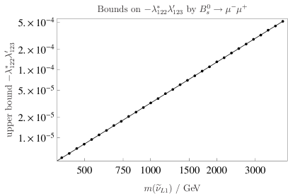
We first present our results for the only case which has been so far considered in the literature for semi-leptonic B𝐵B-meson decays in the context of broken R𝑅R-parity: combinations of couplings which can cause these decays at tree level. In general the tree level diagrams are not the only relevant SUSY contributions. Especially chargino loops can have a non negligible effect as shown in the previous section. However, we ignore these contributions as is usually done in the literature for a moment since they introduce a dependence on several SUSY masses and parameters. Under this assumption, the matrix element is proportional to λλ/mf~2superscript𝜆superscript𝜆superscriptsubscript𝑚~𝑓2\lambda^{*}\lambda^{\prime}/m_{\widetilde{f}}^{2}, i.e. it depends only on the R𝑅RpV couplings and the mass of the propagating sfermion. This scaling is also reflected in our numerical analysis as shown for a representative case on the left in Fig. 5. Our entire results are summarized in Tab. 5. We pick only one representative case for the following discussion and comparison with previous studies. The extracted limits for λi22λi23subscript𝜆𝑖22subscriptsuperscript𝜆𝑖23\lambda_{i22}\lambda^{\prime}_{i23} are

3.25×10¹¹[mν~i]23.25superscript1011superscriptdelimited-[]subscript𝑚subscript~𝜈𝑖2\displaystyle-3.25\times 10^{-11}[m_{\widetilde{\nu}_{i}}]^{2} <λi22λi23<2.51×10¹⁰[mν~i]2,i=1,2,same forλi22λi32formulae-sequenceabsentsubscript𝜆𝑖22subscriptsuperscript𝜆𝑖232.51superscript1010superscriptdelimited-[]subscript𝑚subscript~𝜈𝑖2𝑖12same forsubscript𝜆𝑖22subscriptsuperscript𝜆𝑖32\displaystyle<\lambda_{i22}\lambda^{\prime}_{i23}<2.51\times 10^{-10}[m_{\widetilde{\nu}_{i}}]^{2}\,,\hskip 28.45274pti=1,2,\ \text{same for}\ \lambda_{i22}\lambda^{\prime}_{i32} (43a)
1.15×10¹⁰[mν~i]21.15superscript1010superscriptdelimited-[]subscript𝑚subscript~𝜈𝑖2\displaystyle-1.15\times 10^{-10}[m_{\widetilde{\nu}_{i}}]^{2} <λi22λi13<7.06×10¹¹[mν~i]2,i=1,2,3,same forλi22λi31.formulae-sequenceabsentsubscript𝜆𝑖22subscriptsuperscript𝜆𝑖137.06superscript1011superscriptdelimited-[]subscript𝑚subscript~𝜈𝑖2𝑖123same forsubscript𝜆𝑖22subscriptsuperscript𝜆𝑖31\displaystyle<\lambda_{i22}\lambda^{\prime}_{i13}<7.06\times 10^{-11}[m_{\widetilde{\nu}_{i}}]^{2}\,,\hskip 28.45274pti=1,2,3,\ \text{same for}\ \lambda_{i22}\lambda^{\prime}_{i31}. (43b)

Recently published results for these bounds have been Li:2013fa

|iλi22λi23[mν~i]2|<6.521011,|iλi21λi23[mν~i]2|<7.851011.formulae-sequencesubscript𝑖subscript𝜆𝑖22subscriptsuperscript𝜆𝑖23superscriptdelimited-[]subscript𝑚subscript~𝜈𝑖26.52superscript1011subscript𝑖subscript𝜆𝑖21subscriptsuperscript𝜆𝑖23superscriptdelimited-[]subscript𝑚subscript~𝜈𝑖27.85superscript1011\left|{\sum_{i}\frac{\lambda_{i22}\lambda^{\prime}_{i23}}{[m_{\widetilde{\nu}_{i}}]^{2}}}\right|<6.52\cdot 10^{-11}\,,\hskip 28.45274pt\left|{\sum_{i}\frac{\lambda_{i21}\lambda^{\prime}_{i23}}{[m_{\widetilde{\nu}_{i}}]^{2}}}\right|<7.85\cdot 10^{-11}. (44)

As we pointed out in the introduction, a product like λλsuperscript𝜆superscript𝜆\lambda^{*}\lambda^{\prime} (or λλsuperscript𝜆superscript𝜆\lambda^{\prime*}\lambda^{\prime}) has a phase σ𝜎\sigma relative to the SM contributions. By choosing σ=±1𝜎plus-or-minus1\sigma=\pm 1, we obtain the positive and negative bound given in eqs. (43). For σ=1𝜎1\sigma=-1 constructive interference between the SM and R𝑅RpV contributions appears and we obtain the stronger limit (3.25×10¹¹[mν~i]23.25superscript1011superscriptdelimited-[]subscript𝑚subscript~𝜈𝑖2-3.25\times 10^{-11}[m_{\widetilde{\nu}_{i}}]^{2}), which is comparable to the one in eq. (44) from Ref. Li:2013fa , but slightly better, because we used an updated experimental bound. The reason that the limit for the destructive phase is much weaker is not only the asymmetric bounds in eq. (9), but also based on the different operators which enter the calculation. The RpV𝑅pVR\mathrm{pV} contributions stem only from sneutrino exchange diagrams at tree level, which contribute to the scalar and pseudoscalar coefficients FS,FPsubscript𝐹𝑆subscript𝐹𝑃F_{S},F_{P} introduced in eq. (1). While FSRpV=FPRpVsuperscriptsubscript𝐹𝑆𝑅𝑝𝑉superscriptsubscript𝐹𝑃𝑅𝑝𝑉F_{S}^{RpV}=-F_{P}^{RpV} holds, Bs0μμ¯subscriptsuperscript𝐵0𝑠𝜇¯𝜇B^{0}_{s}\to\mu\bar{\mu} in the SM is determined mainly by the axial vector coefficient FAsubscript𝐹𝐴F_{A}.

Refer to caption
Refer to caption
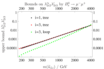
Figure 5: Limits on R𝑅RpV couplings as function of the sfermion mass in the propagator. Left: Bounds for λ122λ123subscript𝜆122subscriptsuperscript𝜆123-\lambda_{122}\lambda^{\prime}_{123} (s𝑠s-channel). Right: Bounds for λ2i2λ2i3subscriptsuperscript𝜆2𝑖2subscriptsuperscript𝜆2𝑖3\lambda^{\prime*}_{2i2}\lambda^{\prime}_{2i3} (t𝑡t-channel). The black dots (i=1𝑖1i=1) and red dots (i=3𝑖3i=3) follow the m~2similar-toabsentsuperscript~𝑚2\sim{\tilde{m}^{2}} scaling. They only contain tree level contributions and SM one-loop contributions. The green dots include the full one-loop SUSY contributions and do not follow this scaling.

Also for λλsuperscript𝜆superscript𝜆\lambda^{\prime}\lambda^{\prime} we find the expected scaling if one neglects other SUSY contributions, see Fig. 5 (right). To demonstrate the effect of the other SUSY loops on this scaling we compare on the right in Fig. 5 the case with and without the other SUSY contributions. One can see that especially for light sfermions this can cause a pronounced difference and leads not only to an off-set but also to a different slope. Hence, if one studies areas in the parameter space of R𝑅RpV SUSY containing light squarks it might not be sufficient to consider just the simplified limits usually discussed in this context, but each point has to be studied carefully.

V.1.2 Indirect Tree Level Results

Indirect Tree Level
λλsuperscript𝜆superscript𝜆\lambda^{\prime*}\lambda^{\prime} λλ>0superscript𝜆superscript𝜆0\lambda^{*\prime}\lambda^{\prime}>0 λλ<0superscript𝜆superscript𝜆0\lambda^{*\prime}\lambda^{\prime}<0
2i2 2i22𝑖22𝑖22i2\ 2i2, i=1,2𝑖12i=1,2 <8.2×10⁵[mu~i2]absent8.2superscript105delimited-[]superscriptsubscript𝑚subscript~𝑢𝑖2<8.2\times 10^{-5}[m_{\widetilde{u}_{i}}^{2}] -
2i3 2i32𝑖32𝑖32i3\ 2i3, i=1,2𝑖12i=1,2 <1.5×10⁵[mu~i2]absent1.5superscript105delimited-[]superscriptsubscript𝑚subscript~𝑢𝑖2<1.5\times 10^{-5}[m_{\widetilde{u}_{i}}^{2}] -
2i2 2i22𝑖22𝑖22i2\ 2i2, i=3𝑖3i=3 <3.1×10⁷[mu~i2]absent3.1superscript107delimited-[]superscriptsubscript𝑚subscript~𝑢𝑖2<3.1\times 10^{-7}[m_{\widetilde{u}_{i}}^{2}] -
2i3 2i32𝑖32𝑖32i3\ 2i3, i=3𝑖3i=3 <6.0×10⁵[mu~i2]absent6.0superscript105delimited-[]superscriptsubscript𝑚subscript~𝑢𝑖2<6.0\times 10^{-5}[m_{\widetilde{u}_{i}}^{2}] -
λλsuperscript𝜆superscript𝜆\lambda^{*}\lambda^{\prime} λλ>0superscript𝜆superscript𝜆0\lambda^{*}\lambda^{\prime}>0 λλ<0superscript𝜆superscript𝜆0\lambda^{*}\lambda^{\prime}<0
i22i12𝑖22𝑖12i22\ i12, i=1,2,3𝑖123i=1,2,3 <3.3×10⁷[mν~i2]absent3.3superscript107delimited-[]superscriptsubscript𝑚subscript~𝜈𝑖2<3.3\times 10^{-7}[m_{\widetilde{\nu}_{i}}^{2}] >2.6×10⁸[mν~i2]absent2.6superscript108delimited-[]superscriptsubscript𝑚subscript~𝜈𝑖2>-2.6\times 10^{-8}[m_{\widetilde{\nu}_{i}}^{2}]
i22i22𝑖22𝑖22i22\ i22, i=1,2,3𝑖123i=1,2,3 <5.1×10⁹[mν~i2]absent5.1superscript109delimited-[]superscriptsubscript𝑚subscript~𝜈𝑖2<5.1\times 10^{-9}[m_{\widetilde{\nu}_{i}}^{2}] >7.9×10⁸[mν~i2]absent7.9superscript108delimited-[]superscriptsubscript𝑚subscript~𝜈𝑖2>-7.9\times 10^{-8}[m_{\widetilde{\nu}_{i}}^{2}]
i22i33𝑖22𝑖33i22\ i33, i=1,2,3𝑖123i=1,2,3 <6.8×10⁸[mν~i2]absent6.8superscript108delimited-[]superscriptsubscript𝑚subscript~𝜈𝑖2<6.8\times 10^{-8}[m_{\widetilde{\nu}_{i}}^{2}] >4.0×10⁹[mν~i2]absent4.0superscript109delimited-[]superscriptsubscript𝑚subscript~𝜈𝑖2>-4.0\times 10^{-9}[m_{\widetilde{\nu}_{i}}^{2}]
i22i21𝑖22𝑖21i22\ i21, i=1,2,3𝑖123i=1,2,3 <3.8×10⁸[mν~i2]absent3.8superscript108delimited-[]superscriptsubscript𝑚subscript~𝜈𝑖2<3.8\times 10^{-8}[m_{\widetilde{\nu}_{i}}^{2}] >2.2×10⁸[mν~i2]absent2.2superscript108delimited-[]superscriptsubscript𝑚subscript~𝜈𝑖2>-2.2\times 10^{-8}[m_{\widetilde{\nu}_{i}}^{2}]
i22i11𝑖22𝑖11i22\ i11, i=1,2,3𝑖123i=1,2,3 <1.0×10⁷[mν~i2]absent1.0superscript107delimited-[]superscriptsubscript𝑚subscript~𝜈𝑖2<1.0\times 10^{-7}[m_{\widetilde{\nu}_{i}}^{2}] >1.8×10⁷[mν~i2]absent1.8superscript107delimited-[]superscriptsubscript𝑚subscript~𝜈𝑖2>-1.8\times 10^{-7}[m_{\widetilde{\nu}_{i}}^{2}]
Table 6: Collection of bounds from decays with sfermions in the propagator which rely on a flavor change in one SM or SUSY loop (’indirect tree level’). We used the input parameters given in Tab. 1. The notation [mf~2]delimited-[]superscriptsubscript𝑚~𝑓2[m_{\widetilde{f}}^{2}] means mf~2/(GeV)2superscriptsubscript𝑚~𝑓2superscriptGeV2m_{\widetilde{f}}^{2}/(\text{Ge}\text{V})^{2}.

There is another class of combinations for SUSY-penguins described in eq. (26) which rely on an additional flavor change in either the SM or another SUSY loop. The results for these couplings are given in Tab. 6. Here, we have included all SUSY corrections present in our benchmark scenario. While the bounds for λλsuperscript𝜆superscript𝜆\lambda^{*}\lambda^{\prime} scale proportional to mν~i2superscriptsubscript𝑚subscript~𝜈𝑖2m_{\widetilde{\nu}_{i}}^{2} to an high accuracy, this holds for the dependence of the limits for λλsuperscript𝜆superscript𝜆\lambda^{*\prime}\lambda^{\prime} on mu~i2superscriptsubscript𝑚subscript~𝑢𝑖2m_{\widetilde{u}_{i}}^{2} only to some extent: the squark masses appear not only in the propagator but also in the important chargino loop. In general the resulting limits are worse than for the pure tree level contributions: for our benchmark point with mν~i1TeVsubscript𝑚subscript~𝜈𝑖1TeVm_{\widetilde{\nu}_{i}}\approx 1~{}\text{Te}\text{V}, the bounds are between 0.330.330.33 and 4×1034superscript1034\times 10^{-3}. Nevertheless, these limits are still competitive with those of direct tree level semi-leptonic decays of other mesons. For instance, the combination λi22λi12superscriptsubscript𝜆𝑖22subscriptsuperscript𝜆𝑖12\lambda_{i22}^{*}\lambda^{\prime}_{i12} is also constrained by searches for K0μμ¯superscript𝐾0𝜇¯𝜇K^{0}\to\mu\bar{\mu}. The tree level limit based on this observable is given by Barbier:2004ez

|λi22λi12|<2.2×10⁷[mν~L2],subscriptsuperscript𝜆𝑖22subscriptsuperscript𝜆𝑖122.2superscript107delimited-[]superscriptsubscript𝑚subscript~𝜈𝐿2\left|{\lambda^{*}_{i22}\lambda^{\prime}_{i12}}\right|<2.2\times 10^{-7}[m_{\widetilde{\nu}_{L}}^{2}]\,, (45)

which we improve on at one side of our asymmetric bound by about one order magnitude.

We don’t give the limits for other parameter combinations of λλsuperscript𝜆superscript𝜆\lambda^{\prime*}\lambda^{\prime} which would in principle also contribute to indirect tree level decays: (2ij)×(2i3)2𝑖𝑗2𝑖3(2ij)\times(2i3) and (2ij)×(2i2)2𝑖𝑗2𝑖2(2ij)\times(2i2) (j2𝑗2j\neq 2). These are partially already constrained by Bd0μμ¯subscriptsuperscript𝐵0𝑑𝜇¯𝜇B^{0}_{d}\to\mu\bar{\mu}. In addition, there is always a superposition of two contributions |λ2i3|2+λ2ijλ2i3superscriptsubscript𝜆2𝑖32subscriptsuperscript𝜆2𝑖𝑗subscript𝜆2𝑖3|\lambda_{2i3}|^{2}+\lambda^{\prime*}_{2ij}\lambda_{2i3} which does not provide a clean environment to derive limits only on just one combination.

V.2 One-Loop Results

One-Loop Level
λλsuperscript𝜆superscript𝜆\lambda^{\prime*}\lambda^{\prime} λλ>0superscript𝜆superscript𝜆0\lambda^{\prime*}\lambda^{\prime}>0 λλ<0superscript𝜆superscript𝜆0\lambda^{\prime*}\lambda^{\prime}<0
Bs,dμ¯μsubscript𝐵𝑠𝑑¯𝜇𝜇B_{s,d}\to\bar{\mu}\mu BXsγ𝐵subscript𝑋𝑠𝛾B\to X_{s}\gamma\, Bs,dμ¯μsubscript𝐵𝑠𝑑¯𝜇𝜇B_{s,d}\to\bar{\mu}\mu BXsγ𝐵subscript𝑋𝑠𝛾B\to X_{s}\gamma\,
3j2 3j3,j=1,2formulae-sequence3𝑗23𝑗3𝑗123j2\ 3j3,\ j=1,2 <2.89absent2.89<2.89 <8.80absent8.80<8.80 Øitalic-Ø\O{} >5.45absent5.45>-5.45
3j2 3j33𝑗23𝑗33j2\ 3j3, j=3𝑗3j=3 <0.49absent0.49<0.49 <2.57absent2.57<2.57 >0.085absent0.085>-0.085 >6.24absent6.24>-6.24
32j 33j,j=1,2formulae-sequence32𝑗33𝑗𝑗1232j\ 33j,\ j=1,2 Øitalic-Ø\O{} <5.28absent5.28<5.28 Øitalic-Ø\O{} >1.15absent1.15>-1.15
32j 33j32𝑗33𝑗32j\ 33j, j=3𝑗3j=3 <11.25absent11.25<11.25 <5.28absent5.28<5.28 Øitalic-Ø\O{} >1.15absent1.15>-1.15
331 333331333331\ 333 <0.45absent0.45<0.45 X𝑋X >0.96absent0.96>-0.96 X𝑋X
i1ji3j𝑖1𝑗𝑖3𝑗i1j\ i3j Øitalic-Ø\O{} X𝑋X Øitalic-Ø\O{} X𝑋X
λ′′λ′′superscript𝜆′′superscript𝜆′′\lambda^{{\prime\prime}*}\lambda^{\prime\prime} λ′′λ′′>0superscript𝜆′′superscript𝜆′′0\lambda^{{\prime\prime}*}\lambda^{\prime\prime}>0 λ′′λ′′<0superscript𝜆′′superscript𝜆′′0\lambda^{{\prime\prime}*}\lambda^{\prime\prime}<0
i12i13,i=1,2formulae-sequence𝑖12𝑖13𝑖12i12\ i13,\ i=1,2 Øitalic-Ø\O{} <0.69absent0.69<0.69 Øitalic-Ø\O{} >2.46absent2.46>-2.46
312 313312313312\ 313 <0.178absent0.178<0.178 <5.00absent5.00<5.00 >0.030absent0.030>-0.030 >6.00absent6.00>-6.00
i21i23,i=1,2formulae-sequence𝑖21𝑖23𝑖12i21\ i23,\ i=1,2 Øitalic-Ø\O{} X𝑋X Øitalic-Ø\O{} X𝑋X
321 323321323321\ 323 <0.162absent0.162<0.162 X𝑋X >0.347absent0.347>-0.347 X𝑋X
Table 7: Collection of bounds for decays at one-loop level for the input parameters given in Tab. 1. Øitalic-Ø\O{} means that the limit is outside the perturbative range, while the couplings marked with X𝑋X don’t contribute to BXsγ𝐵subscript𝑋𝑠𝛾B\to X_{s}\gamma\,. The parameter dependence of the bounds is discussed in detail in the text.

In Tab. 7 we summarize the limits on those RpV couplings which lead to additional one-loop contributions to the neutral B𝐵B-meson decays. In general one can see that in most cases, in which it is possible at all to obtain a limit from the leptonic decays, that the limits are stronger than for the radiative decay. The is the case for couplings which include heavy SM fermions. In contrast BXsγ𝐵subscript𝑋𝑠𝛾B\to X_{s}\gamma\, puts limits on all combination independently of the involved SM fermion of roughly the same order. This different behavior can be understood from eq. (37) in comparison to eq. (38). The obtained limits for BXsγ𝐵subscript𝑋𝑠𝛾B\to X_{s}\gamma\, are in agreement with previous results given in eqs. (39) to (41) but slightly stronger since we included the chargino loops in our analysis.

Since it is not possible to parametrize the limits as a function of the relevant SUSY masses in contrast to the tree level decays, we are going to discuss the dependence on the different masses and parameters in more detail in the following.

V.2.1 One-Loop Results for LQD

(a) Refer to caption (b) Refer to caption
(c) Refer to caption (d) Refer to caption

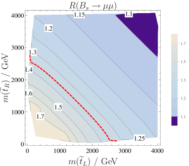
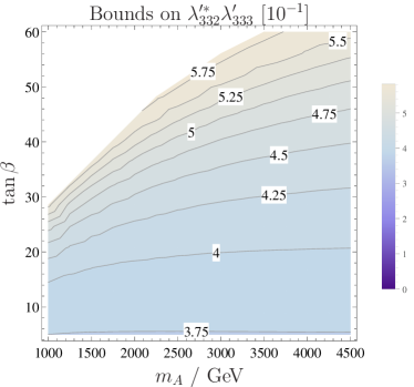
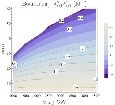
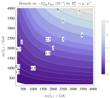
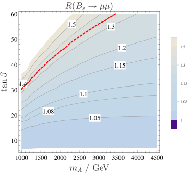
Figure 6: First row: Rssubscript𝑅𝑠R_{s} is plotted in the mAsubscript𝑚𝐴m_{A}tanβ𝛽\tan\beta plane (left, exclusion above the red dashed line) and in the mt~L/Rsubscript𝑚subscript~𝑡𝐿𝑅m_{\widetilde{t}_{L/R}} plane (right, exclusion below the red dashed line) without R𝑅RpV contributions. Second row: The left picture shows the upper bounds on λ332λ333>0subscriptsuperscript𝜆332subscriptsuperscript𝜆3330\lambda^{\prime*}_{332}\lambda^{\prime}_{333}>0 in the mAsubscript𝑚𝐴m_{A}tanβ𝛽\tan\beta plane, the right picture shows the upper bound on λ332λ333<0subscriptsuperscript𝜆332subscriptsuperscript𝜆3330\lambda^{\prime*}_{332}\lambda^{\prime}_{333}<0. All other parameters are fixed to Tab. 1. Note that the bounds are scaled by a factor of 101superscript10110^{-1}.

It is well known that in the MSSM the most important SUSY corrections to Bs0μμsuperscriptsubscript𝐵𝑠0𝜇𝜇B_{s}^{0}\to\mu\mu are due to chargino-loops bsmumu-susy . These loops have a very strong dependence on tanβ𝛽\tan\beta and scale as tan6βproportional-toabsentsuperscript6𝛽\propto\tan^{6}\beta Buras:2002vd . Therefore, we start with a discussion of this effect and check how the bounds for our benchmark point change as a function of tanβ𝛽\tan\beta. The results for each scan are given in a contour plot where the height corresponds to the upper bound of the λλsuperscript𝜆superscript𝜆\lambda^{*\prime}\lambda^{\prime} combination. Note, the contours are rescaled by a factor given in the title of the plot. The variation of the different parameters changes, of course, also the Higgs mass. However, the contribution of a SM-like Higgs to the observables under consideration is negligible. Therefore, it is not necessary to take this effect into account in the following discussions.
Refer to caption
Refer to caption
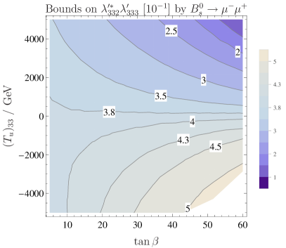
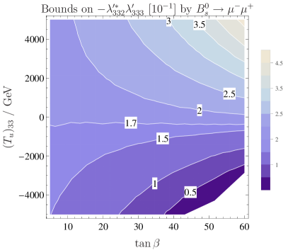
Figure 7: Upper bounds on λ332λ333subscriptsuperscript𝜆332subscriptsuperscript𝜆333\lambda^{\prime*}_{332}\lambda^{\prime}_{333} for a variation of tanβ𝛽\tan\beta and (Tu)33subscriptsubscript𝑇𝑢33(T_{u})_{33}. On the left we assumed λ332λ333>0subscriptsuperscript𝜆332subscriptsuperscript𝜆3330\lambda^{\prime*}_{332}\lambda^{\prime}_{333}>0 and on the right λ332λ333<0subscriptsuperscript𝜆332subscriptsuperscript𝜆3330\lambda^{\prime*}_{332}\lambda^{\prime}_{333}<0. The other parameters are fixed to Tab. 1.

The plots in the first row of Fig. 6 show an exclusion limit for large tanβ𝛽\tan\beta with small mAsubscript𝑚𝐴m_{A} (Fig. 6a, above the red dashed line) and for small stop masses mt~L/Rsubscript𝑚subscript~𝑡𝐿𝑅m_{\widetilde{t}_{L/R}} (Fig. 6b, below the red dashed line) in the absence of any R𝑅RpV contributions. Based on this the bounds on RpV𝑅pVR\mathrm{pV} couplings derived have a strong indirect dependence on tanβ𝛽\tan\beta. While the R𝑅RpV contributions themselve have only a very small dependence on tanβ𝛽\tan\beta, the enhancement of the other SUSY loops can change the limits signficantly: in the case of contructive interference (Fig. 6d) the bounds improve by about one order of magnitude between tanβ=5𝛽5\tan\beta=5 and 50. For destructive interference (Fig. 6c) the bounds are relaxed by a factor of about 1.5.

The variation of tanβ𝛽\tan\beta together with the trilinear soft-breaking parameter Tusubscript𝑇𝑢T_{u} is shown in Fig. 7. The more negative the parameter (Tu)33subscriptsubscript𝑇𝑢33(T_{u})_{33}, the larger is the mass splitting between the stop squarks and the lighter is the lightest stop squark. Hence, the limits for the couplings increase (decrease) for decreasing (Tu)33subscriptsubscript𝑇𝑢33(T_{u})_{33} in the case of destructive (constructive) interference. The original benchmark point has (Tu)33=3.17TeVsubscriptsubscript𝑇𝑢333.17TeV(T_{u})_{33}=-3.17~{}\text{Te}\text{V} and tanβ=42𝛽42\tan\beta=42. These are the values which we use in all upcoming figures.

We turn now to a discussion of the impact of the different masses appearing in the loop. In general, the case λijXλij3subscriptsuperscript𝜆𝑖𝑗𝑋superscriptsubscript𝜆𝑖𝑗3\lambda^{*\prime}_{ijX}\lambda_{ij3}^{\prime} (X=1,2𝑋12X=1,2) is sensitive to different squark and slepton masses. To make this dependence visible we have varied independently the entries mL,ii2superscriptsubscript𝑚𝐿𝑖𝑖2m_{L,ii}^{2} and mQ,jj2superscriptsubscript𝑚𝑄𝑗𝑗2m_{Q,jj}^{2} of the soft-breaking masses. The masses that appear in the plots are running DR¯¯DR\overline{\mathrm{DR}} masses. If a mass is called mt~Lsubscript𝑚subscript~𝑡𝐿m_{\widetilde{t}_{L}}, this actually means the mass of the mass eigenstate t~isubscript~𝑡𝑖\widetilde{t}_{i} which is mainly t~Lsubscript~𝑡𝐿\widetilde{t}_{L}–like according to the mixing matrix.

(a) Refer to caption (b) Refer to caption
(c) Refer to caption (d) Refer to caption

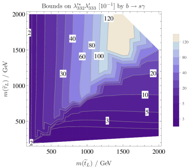
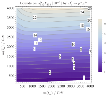
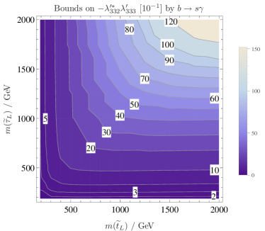
Figure 8: Bounds for λ332λ333subscriptsuperscript𝜆332subscriptsuperscript𝜆333\lambda^{\prime*}_{332}\lambda^{\prime}_{333} couplings at one-loop with a variation of the masses of t~Lsubscript~𝑡𝐿\widetilde{t}_{L} and τ~Lsubscript~𝜏𝐿\widetilde{\tau}_{L}. First row: Bounds for λ332λ333<0subscriptsuperscript𝜆332subscriptsuperscript𝜆3330\lambda^{\prime*}_{332}\lambda^{\prime}_{333}<0 (constructive interference at Bs0μμ¯subscriptsuperscript𝐵0𝑠𝜇¯𝜇B^{0}_{s}\to\mu\bar{\mu}). Second row: Bounds for λ332λ333>0subscriptsuperscript𝜆332subscriptsuperscript𝜆3330\lambda^{\prime*}_{332}\lambda^{\prime}_{333}>0 (destructive interference for Bs0μμ¯subscriptsuperscript𝐵0𝑠𝜇¯𝜇B^{0}_{s}\to\mu\bar{\mu}). The other parameters are fixed to Tab. 1.

As an example, we show the upper limit on a specific combination with only third generation sfermions, λ332λ333subscriptsuperscript𝜆332subscriptsuperscript𝜆333\lambda^{\prime*}_{332}\lambda^{\prime}_{333}. In Fig. 8 the upper limits are shown as a function of the masses of the involved top squark (t~Lsubscript~𝑡𝐿\widetilde{t}_{L}) and stau (τLsubscript𝜏𝐿\tau_{L}). The first row corresponds to a phase 11-1 (constructive interference for Bs0μμ¯subscriptsuperscript𝐵0𝑠𝜇¯𝜇B^{0}_{s}\to\mu\bar{\mu}) and the second row to a phase +11+1 (destructive interference for Bs0μμ¯subscriptsuperscript𝐵0𝑠𝜇¯𝜇B^{0}_{s}\to\mu\bar{\mu}). The left column shows the bounds from the decay BXsγ𝐵subscript𝑋𝑠𝛾B\to X_{s}\gamma\,, which turn out to be weaker than those from the decay Bs0μμ¯subscriptsuperscript𝐵0𝑠𝜇¯𝜇B^{0}_{s}\to\mu\bar{\mu} (right column). Interestingly, the choice of sign for constructive interference in Bs0μμ¯subscriptsuperscript𝐵0𝑠𝜇¯𝜇B^{0}_{s}\to\mu\bar{\mu} is destructive interference for BXsγ𝐵subscript𝑋𝑠𝛾B\to X_{s}\gamma\, and vice versa. In the case of constructive interference a similar mass dependence can be observed. We can see in Fig. 8d that there is almost no stop mass dependence, except for heavy stau masses and light stop masses. This can be explained by the scaling behavior in eq. (37). The τt~𝜏~𝑡\tau\widetilde{t} loops become competitive with the τ~t~𝜏𝑡\widetilde{\tau}t loops only if mτ/mtmt~2/mτ~2subscript𝑚𝜏subscript𝑚𝑡subscriptsuperscript𝑚2~𝑡subscriptsuperscript𝑚2~𝜏m_{\tau}/m_{t}\approx m^{2}_{\widetilde{t}}/m^{2}_{\widetilde{\tau}}, which applies to the region of the plot where we see a mτ~subscript𝑚~𝜏m_{\widetilde{\tau}} dependence.

Refer to caption
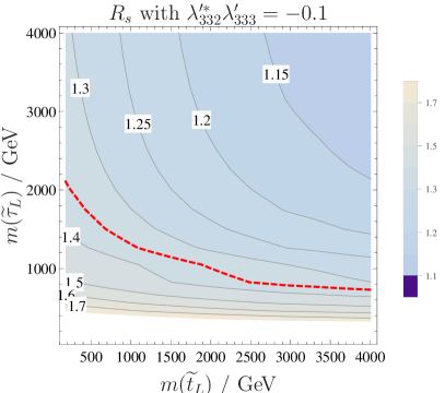
Figure 9: Rssubscript𝑅𝑠R_{s} for fixed λ332λ333=0.1subscriptsuperscript𝜆332subscriptsuperscript𝜆3330.1\lambda^{\prime*}_{332}\lambda^{\prime}_{333}=-0.1 as function of m(t~L)𝑚subscript~𝑡𝐿m(\tilde{t}_{L}) and m(τ~L)𝑚subscript~𝜏𝐿m(\tilde{\tau}_{L}). The area below the red line is excluded by the current experimental limits.

Finally, we can also check how well Bs0μμ¯subscriptsuperscript𝐵0𝑠𝜇¯𝜇B^{0}_{s}\to\mu\bar{\mu} has to be measured to constrain the squark masses for a given order of R𝑅RpV couplings. This is done in Fig. 9 where we plot Rssubscript𝑅𝑠R_{s} as function of the involved masses assuming λ332λ333=0.1subscriptsuperscript𝜆332subscriptsuperscript𝜆3330.1\lambda^{\prime*}_{332}\lambda^{\prime}_{333}=-0.1. The region below the red dashed line (small squark masses) would then be excluded by the current upper bound on BR(Bs0μμ¯)BRsubscriptsuperscript𝐵0𝑠𝜇¯𝜇\text{BR}(B^{0}_{s}\to\mu\bar{\mu})\,. Obviously, if both sfermions are heavier than 2 TeV, the entire contribution is of at most 20% of the SM contribution. This is the same order of magnitude as the theoretical uncertainty which we have assumed.

V.2.2 One-Loop Results for UDD
Refer to caption
Refer to caption
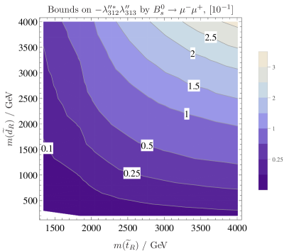
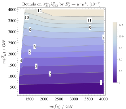
Figure 10: Similar to Fig. 8 but for pairs of baryon number violating couplings. On the left we used λ312′′λ313′′>0subscriptsuperscript𝜆′′312subscriptsuperscript𝜆′′3130\lambda^{\prime\prime*}_{312}\lambda^{\prime\prime}_{313}>0 and on the right λ312′′λ313′′<0subscriptsuperscript𝜆′′312subscriptsuperscript𝜆′′3130\lambda^{\prime\prime*}_{312}\lambda^{\prime\prime}_{313}<0.

When considering UDD couplings, the masses appearing in the loops from RpV𝑅pVR\mathrm{pV} contributions are the right handed squarks, d~Ri,u~Risubscript~𝑑𝑅𝑖subscript~𝑢𝑅𝑖\widetilde{d}_{Ri},\widetilde{u}_{Ri}. The stop mass also influences the chargino contribution to Bs,d0μμ¯subscriptsuperscript𝐵0𝑠𝑑𝜇¯𝜇B^{0}_{s,d}\to\mu\bar{\mu}\,, which has already been shown in Fig. 6 (top right) for vanishing RpV𝑅pVR\mathrm{pV} contributions. When RpV𝑅pVR\mathrm{pV} contributions are considered, they come “on top”. Thus we expect to see slightly better constraints than in the LQD case. Indeed, in the case of constructive interference (Fig. 10, right side) the constraints are of the order 102superscript10210^{-2}. Like in the LQD case, there is almost no down squark mass dependence in Fig. 10 (left), except for low stop masses and high d~Rsubscript~𝑑𝑅\widetilde{d}_{R} masses. In contrast, the limits obtained by BXsγ𝐵subscript𝑋𝑠𝛾B\to X_{s}\gamma\, show nearly the same dependence on m(d~R)𝑚subscript~𝑑𝑅m(\widetilde{d}_{R}) and m(t~R)𝑚subscript~𝑡𝑅m(\widetilde{t}_{R}) as depicted on the left hand side of Fig. 10. In contrast to LQD there is positive interference for Bs,d0μμ¯subscriptsuperscript𝐵0𝑠𝑑𝜇¯𝜇B^{0}_{s,d}\to\mu\bar{\mu}\, in the case of λ′′λ′′<0superscript𝜆′′superscript𝜆′′0\lambda^{\prime\prime*}\lambda^{\prime\prime}<0 and destructive interference for positive couplings. BXsγ𝐵subscript𝑋𝑠𝛾B\to X_{s}\gamma\, shows again exactly the opposite behavior.

VI Conclusion

We have presented the first one-loop analysis for Bs,d0μμ¯subscriptsuperscript𝐵0𝑠𝑑𝜇¯𝜇B^{0}_{s,d}\to\mu\bar{\mu}\, in the MSSM with broken R𝑅R-parity. All combinations of couplings between the operators λ𝐋𝐋𝐄𝜆𝐋𝐋𝐄\lambda{\bf LLE} and λ𝐋𝐐𝐃superscript𝜆𝐋𝐐𝐃\lambda^{\prime}{\bf LQD}, as well as λ′′𝐔𝐃𝐃superscript𝜆′′𝐔𝐃𝐃\lambda^{\prime\prime}{\bf UDD} have been considered. We have extracted updated limits on combinations which can trigger Bs,d0μμ¯superscriptsubscript𝐵𝑠𝑑0𝜇¯𝜇B_{s,d}^{0}\to\mu\bar{\mu} either at tree or one-loop level for one benchmark point and discussed the dependence of these limits on the different parameters.

In this context we have pointed out that a tree level analysis alone might not be sufficient but the bounds and the general behavior can change when including loop-effects due to other SUSY particles. In addition, we presented a set of couplings which lead to ‘SUSY penguins’. These diagrams rely on an additional flavor change due to the SM or another SUSY loop. Despite this additional suppression the obtained limits can even be stronger than the ones based on direct tree level decays of other mesons because of the strong experimental limits on the B𝐵B-meson sector. At one-loop level we have shown that only couplings can be constrained by semi-leptonic decays if heavy standard model fermions are involved, i.e. the best limits are stemming from loops involving top quarks. However, even there couplings of O(1)𝑂1O(1) are still in agreement with all observables for SUSY masses in the TeV range and moderate values of tanβ𝛽\tan\beta. R𝑅RpV couplings involving only light SM fermions are not constrained at all by the current measurements of Bs,d0μμ¯subscriptsuperscript𝐵0𝑠𝑑𝜇¯𝜇B^{0}_{s,d}\to\mu\bar{\mu}\,. This is different to BXsγ𝐵subscript𝑋𝑠𝛾B\to X_{s}\gamma\, where the obtained limits are independent of the generation of the SM particles. Furthermore, we have also shown that the dependence on the phase of the R𝑅RpV couplings is opposite between Bs,d0μμ¯subscriptsuperscript𝐵0𝑠𝑑𝜇¯𝜇B^{0}_{s,d}\to\mu\bar{\mu}\, and BXsγ𝐵subscript𝑋𝑠𝛾B\to X_{s}\gamma\,, i.e. depending on the sign one has destructive interference between the SM and R𝑅RpV for one observable and constructive for the other.

Acknowledgements

We thank Werner Porod and Manuel Krauss for helpful discussions.

References

  • (1) ATLAS Collaboration, G. Aad et al., “Search for squarks and gluinos with the ATLAS detector in final states with jets and missing transverse momentum using 4.7 fb1𝑓superscript𝑏1fb^{-}1 of sqrt(s) = 7 TeV proton-proton collision data,” [arXiv:1208.0949 [hep-ex]]
  • (2) CMS Collaboration, S. Chatrchyan et al., “Search for supersymmetry in hadronic final states using MT2 in pp𝑝𝑝pp collisions at s=7𝑠7\sqrt{s}=7 TeV,” JHEP 1210 (2012) 018, [arXiv:1207.1798 [hep-ex]]
  • (3) CMS Collaboration, “Search for supersymmetery in final states with missing transverse momentum and 0, 1, 2, or 3absent3\geq 3 b jets with CMS,”.
  • (4) CMS Collaboration, “Search for supersymmetry with the razor variables at CMS,”.
  • (5) CMS Collaboration, Collaboration, S. Chatrchyan et al., “Search for new physics in the multijet and missing transverse momentum final state in proton-proton collisions at s=7𝑠7\sqrt{s}=7 TeV,” [arXiv:1207.1898 [hep-ex]]
  • (6) P. Bechtle, T. Bringmann, K. Desch, H. Dreiner, M. Hamer, C. Hensel, M. Krämer and N. Nguyen et al., JHEP 1206 (2012) 098 [arXiv:1204.4199 [hep-ph]].
  • (7) D. Ghosh, M. Guchait, S. Raychaudhuri and D. Sengupta, Phys. Rev. D 86 (2012) 055007 [arXiv:1205.2283 [hep-ph]].
  • (8) O. Buchmueller, R. Cavanaugh, M. Citron, A. De Roeck, M. J. Dolan, J. R. Ellis, H. Flacher and S. Heinemeyer et al., Eur. Phys. J. C 72 (2012) 2243 [arXiv:1207.7315].
  • (9) G. Aad et al. [ATLAS Collaboration], Phys. Lett. B 716, 1 (2012) [arXiv:1207.7214 [hep-ex]].
  • (10) S. Chatrchyan et al. [CMS Collaboration], Phys. Lett. B 716, 30 (2012) [arXiv:1207.7235 [hep-ex]].
  • (11) A. Arbey, M. Battaglia, A. Djouadi and F. Mahmoudi, [arXiv:1211.4004 [hep-ph]]. M. W. Cahill-Rowley, J. L. Hewett, A. Ismail and T. G. Rizzo, [arXiv:1211.1981 [hep-ph]]. S. S. AbdusSalam, [arXiv:1211.0999 [hep-ph]]. H. Baer and J. List, [arXiv:1205.6929 [hep-ph]]. M. Carena, J. Lykken, S. Sekmen, N. R. Shah and C. E. M. Wagner, Phys. Rev. D 86, 075025 (2012) [arXiv:1205.5903 [hep-ph]].
  • (12) L. J. Hall and M. Suzuki, Nucl. Phys. B 231, 419 (1984).
  • (13) B. C. Allanach, A. Dedes and H. K. Dreiner, Phys. Rev. D 69 (2004) 115002 [Erratum-ibid. D 72 (2005) 079902] [hep-ph/0309196]. H. K. Dreiner, In *Kane, G.L. (ed.): Perspectives on supersymmetry II* 565-583 [hep-ph/9707435]. G. Bhattacharyya, In *Tegernsee 1997, Beyond the desert 1997* 194-201 [hep-ph/9709395].
  • (14) R. Barbier, C. Berat, M. Besancon, M. Chemtob, A. Deandrea, E. Dudas, P. Fayet and S. Lavignac et al., Phys. Rept.  420, 1 (2005) [hep-ph/0406039].
  • (15) H. K. Dreiner and T. Stefaniak, Phys. Rev. D 86 (2012) 055010 [arXiv:1201.5014 [hep-ph]]. H. K. Dreiner and G. G. Ross, Nucl. Phys. B 365 (1991) 597. M. Asano, K. Rolbiecki and K. Sakurai, [arXiv:1209.5778 [hep-ph]]. B. C. Allanach and B. Gripaios, JHEP 1205 (2012) 062 [arXiv:1202.6616 [hep-ph]]. H. K. Dreiner, S. Grab and T. Stefaniak, Phys. Rev. D 84 (2011) 035023 [arXiv:1102.3189 [hep-ph]].
  • (16) R. Franceschini and R. Torre, Eur. Phys. J. C 73 (2013) 2422 [arXiv:1212.3622 [hep-ph]].
  • (17) J. A. Evans and Y. Kats, JHEP 1304 (2013) 028 [arXiv:1209.0764 [hep-ph]].
  • (18) H. K. Dreiner, F. Staub, A. Vicente and W. Porod, Phys. Rev. D 86 (2012) 035021 [arXiv:1205.0557 [hep-ph]].
  • (19) R. Barbieri and G. F. Giudice, Phys. Lett. B 309 (1993) 86 [hep-ph/9303270].
  • (20) M. Misiak and M. Steinhauser, Nucl. Phys. B 764 (2007) 62 [hep-ph/0609241];
  • (21) M. Misiak, H. M. Asatrian, K. Bieri, M. Czakon, A. Czarnecki, T. Ewerth, A. Ferroglia and P. Gambino et al., Phys. Rev. Lett.  98 (2007) 022002 [hep-ph/0609232]; T. Hurth, E. Lunghi and W. Porod, Nucl. Phys. B 704 (2005) 56 [hep-ph/0312260]; M. Misiak and M. Steinhauser, Nucl. Phys. B 683 (2004) 277 [hep-ph/0401041]; C. Bobeth, P. Gambino, M. Gorbahn and U. Haisch, JHEP 0404 (2004) 071 [hep-ph/0312090]; H. K. Dreiner, Mod. Phys. Lett. A 3 (1988) 867.
  • (22) P. Gambino and M. Misiak, Nucl. Phys. B 611, 338 (2001) [hep-ph/0104034].
  • (23) C. -S. Huang, W. Liao and Q. -S. Yan, Phys. Rev. D 59 (1999) 011701 [hep-ph/9803460]. K. S. Babu and C. F. Kolda, Phys. Rev. Lett.  84 (2000) 228 [hep-ph/9909476]. C. Bobeth, T. Ewerth, F. Kruger and J. Urban, Phys. Rev. D 64 (2001) 074014 [hep-ph/0104284]. A. Dedes, H. K. Dreiner and U. Nierste, Phys. Rev. Lett.  87 (2001) 251804 [hep-ph/0108037]. A. Dedes, J. Rosiek and P. Tanedo, Phys. Rev. D 79 (2009) 055006 [arXiv:0812.4320 [hep-ph]]; P. H. Chankowski and L. Slawianowska, Phys. Rev. D 63 (2001) 054012 [hep-ph/0008046].
  • (24) B. de Carlos and P. L. White, Phys. Rev. D 55 (1997) 4222 [hep-ph/9609443].
  • (25) O. C. W. Kong and R. D. Vaidya, Phys. Rev. D 71 (2005) 055003 [hep-ph/0403148].
  • (26) H. K. Dreiner, M. Krämer and B. O’Leary, Phys. Rev. D 75, 114016 (2007) [hep-ph/0612278].
  • (27) C. Li, C. -D. Lu and X. -D. Gao, [arXiv:1301.3445 [hep-ph]].
  • (28) G. Yeghiyan, arXiv:1305.0852 [hep-ph].
  • (29) F. Staub, Computer Physics Communications 184, pp. 1792 (2013) [arXiv:1207.0906 [hep-ph]]. F. Staub, Comput. Phys. Commun.  182 (2011) 808 [arXiv:1002.0840 [hep-ph]]. F. Staub, Comput. Phys. Commun.  181 (2010) 1077 [arXiv:0909.2863 [hep-ph]]. F. Staub, [arXiv:0806.0538 [hep-ph]].
  • (30) W. Porod and F. Staub, Comput. Phys. Commun.  183 (2012) 2458 [arXiv:1104.1573 [hep-ph]]. W. Porod, Comput. Phys. Commun.  153 (2003) 275 [hep-ph/0301101].
  • (31) H. Dreiner, K. Nickel, W. Porod and F. Staub, [arXiv:1212.5074 [hep-ph]].
  • (32) A. Dedes, J. Rosiek and P. Tanedo, Phys. Rev. D 79 (2009) 055006 [arXiv:0812.4320 [hep-ph]].
  • (33) A. J. Buras, J. Girrbach, D. Guadagnoli and G. Isidori, [arXiv:1208.0934 [hep-ph]].
  • (34) G. Raven [LHCb Collaboration], arXiv:1212.4140 [hep-ex].
  • (35) A. J. Buras, R. Fleischer, J. Girrbach and R. Knegjens, [arXiv:1303.3820 [hep-ph]].
  • (36) LHCb Collaboration: R. Aaij and many more, Phys. Rev. Lett.  110 (2013) 021801 [arXiv:1211.2674 [hep-ex]].
  • (37) LHCb Collaboration: R. Aaij, B. Adeva, and many more, arXiv:1307.5024
  • (38) U. Haisch and F. Mahmoudi, JHEP 1301, 061 (2013) [arXiv:1210.7806 [hep-ph]].
  • (39) J. Beringer et al. [Particle Data Group Collaboration], Phys. Rev. D 86, 010001 (2012).
  • (40) H. K. Dreiner and M. Thormeier, Phys. Rev. D 69, 053002 (2004) [hep-ph/0305270].
  • (41) H. K. Dreiner, K. Nickel, F. Staub and A. Vicente, Phys. Rev. D 86, 015003 (2012) [arXiv:1204.5925 [hep-ph]].
  • (42) E. Lunghi and J. Matias, JHEP 0704 (2007) 058 [hep-ph/0612166].
  • (43) F. Staub, T. Ohl, W. Porod and C. Speckner, Comput. Phys. Commun.  183, 2165 (2012) [arXiv:1109.5147 [hep-ph]].
  • (44) M. W. Cahill-Rowley, J. L. Hewett, A. Ismail, M. E. Peskin and T. G. Rizzo, [arXiv:1305.2419 [hep-ph]].
  • (45) C. F. Berger, J. S. Gainer, J. L. Hewett and T. G. Rizzo, JHEP 0902, 023 (2009) [arXiv:0812.0980 [hep-ph]].
  • (46) J. E. Camargo-Molina, B. O’Leary, W. Porod and F. Staub, arXiv:1307.1477 [hep-ph].
  • (47) A. J. Buras, P. H. Chankowski, J. Rosiek and L. Slawianowska, Nucl. Phys. B 659, 3 (2003) [hep-ph/0210145].