Qatar-1: indications for possible transit timing variations

Abstract

Aims. Variations in the timing of transiting exoplanets provide a powerful tool detecting additional planets in the system. Thus, the aim of this paper is to discuss the plausibility of transit timing variations on the Qatar-1 system by means of primary transit light curves analysis. Furthermore, we provide an interpretation of the timing variation.

Methods. We observed Qatar-1 between March 2011 and October 2012 using the 1.2 m OLT telescope in Germany and the 0.6 m PTST telescope in Spain. We present 26 primary transits of the hot Jupiter Qatar-1b. In total, our light curves cover a baseline of 18 months.

Results. We report on indications for possible long-term transit timing variations (TTVs). Assuming that these TTVs are true, we present two different scenarios that could explain them. Our reported $\sim$ 190 days TTV signal can be reproduced by either a weak perturber in resonance with Qatar-1b, or by a massive body in the brown dwarf regime. More observations and radial velocity monitoring are required to better constrain the perturber’s characteristics. We also refine the ephemeris of Qatar-1b, which we find to be $T_{0}=2456157.42204\pm 0.0001$ $\mathrm{BJD}_{\mathrm{TDB}}$ and $P=1.4200246\pm 0.0000007$ days, and improve the system orbital parameters.

1 Introduction

The discovery of Neptune in 1846 was a milestone in astronomy. The position at which the planet was detected by J. G. Galle had been predicted – independently – by U.J. Le Verrier and J. C. Adams, who attributed the observed irregularities of Uranus’ orbit to the gravitational attraction of another perturbing body outside Uranus’ radius. Thus, Neptune became the first planet to be predicted by celestial mechanics before it was directly observed.

Similar to the case of Neptune, in the realm of exoplanets an additional planet or exomoon can reveal itself by its gravitational influence on the orbital elements of the observed planet. Most notably, for transiting planets a perturber is expected to induce short-term transit timing variations (TTVs) (Holman & Murray (2005); Agol et al. (2005)); because timing measurements can be carried out quite accurately, the TTV searches are quite sensitive, and it is possible to detect additional objects in the stellar system and to derive their properties with TTVs.

The detection of TTVs in ground-based measurements requires both a sufficiently long baseline and good phase coverage. The search for planets by TTVs has been a major activity in ground-based exoplanet research. So far, TTVs have been claimed in WASP-3b (Maciejewski et al., 2010), WASP-10b (Maciejewski et al., 2011), WASP-5b (Fukui et al., 2011), HAT-P-13 (Pál et al. (2011), Nascimbeni et al. (2011), but see Fulton et al. (2011)), and OGLE-111b (Díaz et al. (2008), but see Adams et al. (2010)).

In recent years, the search for TTVs in extrasolar planetary systems has entered a new era, marked by the advent of the space-based observatories CoRoT and Kepler, which provide photometry of unprecedented accuracy. On one hand, the Kepler team has already presented more than 40 TTVs in exoplanetary systems, such as Kepler-9 (Holman et al. (2010)), Kepler-11 (Lissauer et al., 2011), Kepler-19 Ballard et al. (2011), Kepler-18 (Cochran et al., 2011), and Kepler 29, 30, 31 and 32 (Fabrycky et al., 2012). On the other hand, Steffen et al. (2012) searched for planetary companions orbiting hot-Jupiter planet candidates and found that most of the systems show no significant TTV signal. Yet, the Kepler satellite observes only a small area of the sky and has a limited lifetime, thus TTV will continue to play a major role also in ground-based studies.

The transiting Jovian planet Qatar-1b was discovered by Alsubai et al. (2011) as the first planet found within The Qatar Exoplanet Survey. Qatar-1A is an old ($>4$ Gy) K3V star with 0.85 M_⊙ and 0.82 R_⊙, orbited by a close-in ($0.023$ AU) planet with a mass of $1.1$ M_J and a period of $1.42$ d. Qatar-1b has a radius of $1.16$ R_J and an inclination angle of $83.47^{\circ}$, implying a nearly grazing transit. Therefore Qatar-1 offers an outstanding opportunity to search for TTVs for several reasons: Its large inclination and close-in orbit yield a high-impact parameter, making the shape and timing of the transit sensitive to variations of the orbital parameters. Its large radius and short orbital period allow for the study of a large number of deep transits over hundreds of epochs.

We have therefore observed transits in Qatar-1b over the past few years, which we describe here. We specifically describe the observational setup in section 2 as well as the data reduction process. We subsequently present the details of our light curve analysis and transit modeling in Sect. 3 and describe our TTV analysis in section 4. We interpret our results in Section 5, where we present different dynamical scenarios that were tested to suggest the existence of an additional body in the system. In Section 6 we conclude.

2 Observations and data reduction

Our observations comprise 18 transits of Qatar-1 obtained using the 1.2 m Oskar-Lühning telescope (OLT) at Hamburg Observatory, Germany, and 8 transits using the 0.6 m Planet Transit Study Telescope (PTST) at the Mallorca Observatory in Spain.

The OLT data were taken between March 2011 and October 2012 using an Apogee Alta U9000 CCD with a $9^{\prime}\times 9^{\prime}$ field of view. Binning was usually $4\times 4$, but the first transit observations were taken in a $2\times 2$ configuration. The binning was increased to reduce individual exposure times. The data were obtained with typical exposure times between 45 and 300 seconds depending on the night quality, the binning configuration, and the star’s altitude. All exposures were obtained using a Johnson-Cousins Schuler R filter. Because Qatar-1 is circumpolar at Hamburg’s latitude, typical airmass values range from 1 up to 1.9, while the average seeing value is 2.5 arcsec.

The PTST data were taken between May and August 2012 using a Santa Barbara CCD with a $30^{\prime}\times 30^{\prime}$ field of view in a $3\times 3$ binning and a Baade R-band filter setup. The exposure times range from 50 to 90 seconds. The observations were obtained with airmass values between 1.1 and 3 and typical seeing values of 2 arcsec. In Table 1 we summarize the main characteristics of our observations obtained at both sites. Combining OLT and PTST data, the observations cover a total of 416 epochs.

Table 1: Summary of our observations carried out with OLT (top) and PTST (bottom) specifying epoch, exposure time ET, filter configuration F, number of data points NoP, airmass and transit coverage (TC); a description of the transit coding is detailed in the footnote of this table. Epochs are counted relative to the best-fitting transit. Transits observed simultaneously with both telescopes are marked in boldface.

Date	Epoch	ET	F	NoP	Airmass	TC
		(s)
OLT
2011 March 19	-364	202	R1	29	1.83$\leavevmode\nobreak\ \rightarrow\leavevmode\nobreak\$1.40	- IBE -
2011 March 26	-359	296	R1	28	1.45$\leavevmode\nobreak\ \rightarrow\leavevmode\nobreak\$1.19	OIBE -
2011 May 22	-319	173	R1	48	1.60$\leavevmode\nobreak\ \rightarrow\leavevmode\nobreak\$1.18	OIBEO
2011 May 29	-314	58	R1	72	1.19$\leavevmode\nobreak\ \rightarrow\leavevmode\nobreak\$1.08	- - BEO
2011 July 5	-288	82	R1	78	1.13$\leavevmode\nobreak\ \rightarrow\leavevmode\nobreak\$1.03	- - BEO
2011 July 15	-281	136	R1	86	1.21$\leavevmode\nobreak\ \rightarrow\leavevmode\nobreak\$1.02	- - BEO
2011 August 1st	-269	68	R1	108	1.12$\leavevmode\nobreak\ \rightarrow\leavevmode\nobreak\$1.02	OIBEO
2011 August 28	-250	80	R1	42	1.02$\leavevmode\nobreak\ \rightarrow\leavevmode\nobreak\$1.04	- - BEO
2011 October 1st	-226	79	R1	136	1.12$\leavevmode\nobreak\ \rightarrow\leavevmode\nobreak\$1.02	OIBEO
2012 April 21	-83	141	R1	97	1.73$\leavevmode\nobreak\ \rightarrow\leavevmode\nobreak\$1.18	OIBEO
2012 April 24	-81	90	R1	40	1.80$\leavevmode\nobreak\ \rightarrow\leavevmode\nobreak\$1.61	- - BEO
2012 May 1st	-76	70	R1	177	1.71$\leavevmode\nobreak\ \rightarrow\leavevmode\nobreak\$1.18	OIBEO
2012 June 17	-43	53	R1	61	1.39$\leavevmode\nobreak\ \rightarrow\leavevmode\nobreak\$1.21	- - - EO
2012 July 1st	-33	76	R1	112	1.12$\leavevmode\nobreak\ \rightarrow\leavevmode\nobreak\$1.02	OIB - -
2012 August 17	0	50	R1	425	1.12$\leavevmode\nobreak\ \rightarrow\leavevmode\nobreak\$1.14	OIBEO
2012 September 13	19	64	R1	124	1.05$\leavevmode\nobreak\ \rightarrow\leavevmode\nobreak\$1.04	OI - - O
2012 September 30	31	59	R1	100	1.04$\leavevmode\nobreak\ \rightarrow\leavevmode\nobreak\$1.14	- IBEO
2012 October 30	52	52	R1	275	1.03$\leavevmode\nobreak\ \rightarrow\leavevmode\nobreak\$1.16	OIBEO
PTST
2012 February 27	-121	90	R2	109	3.00$\leavevmode\nobreak\ \rightarrow\leavevmode\nobreak\$1.47	OIBEO
2012 May 11	-69	59	R2	183	2.84$\leavevmode\nobreak\ \rightarrow\leavevmode\nobreak\$1.30	OIBEO
2012 May 28	-57	90	R2	106	2.00$\leavevmode\nobreak\ \rightarrow\leavevmode\nobreak\$1.18	OIBEO
2012 June 17	-43	40	R2	168	1.86$\leavevmode\nobreak\ \rightarrow\leavevmode\nobreak\$1.34	- - BEO
2012 July 4	-31	70	R2	80	1.50$\leavevmode\nobreak\ \rightarrow\leavevmode\nobreak\$1.15	OIBEO
2012 July 14	-24	60	R2	86	1.42$\leavevmode\nobreak\ \rightarrow\leavevmode\nobreak\$1.22	- - - EO
2012 July 31	-12	60	R2	133	1.32$\leavevmode\nobreak\ \rightarrow\leavevmode\nobreak\$1.11	OIBEO
2012 August 17	0	40	R2	182	1.22$\leavevmode\nobreak\ \rightarrow\leavevmode\nobreak\$1.23	OIBEO

Calibration images such as bias and flat fields were obtained on each observing night. We used the IRAF task ccdproc for bias subtraction and flat-fielding on the individual data sets, followed by the task apphot to carry out aperture photometry on all images including individual photometric errors. We measured fluxes using different apertures centered on the target star and six more stars with a similar brightness as Qatar-1, which are present in both field of views. The apparent brightness of the reference star chosen to produce the differential light curves is very close to Qatar-1. Multiband photometry of the same field of view reveals no significant difference between both stars as a function of photometric color, either suggesting that they are of similar spectral type. This minimizes any atmospheric extinction residuals on the differential light curves, and in addition, the apparent proximity of the two stars ($\sim$2 arcmin) minimizes systematic effects related to vignetting, comatic aberration, or CCD temperature gradients, which all increase with increasing distance from the telescope’s optical axis (i.e., the center of the chip). We also checked the constancy of the reference star against the other five comparison stars and chose as final aperture the one that minimized the scatter in the resulting light curves. The differential light curves were then produced by dividing the flux of the target star by that of the reference star.

Typical sky brightness values per binned pixel were of about 3500 counts for OLT, and 2000 for PTST. Figure 1 shows the PTST field of view (light background) superposed on the field of view of OLT (dark background). Qatar-1 lies at the center of the field of view, marked with a large red circle. The five comparison stars are indicated with green squares and the reference star, indicated with a small blue circle, is the one used to produce the differential light curves.

After the reduction process, we fitted a straight line to the out-of-transit data points to correct for any residual systematic trend and to normalize the differential light curves. It is worth mentioning that we calculated the timing offsets using both raw and normalized data. We therefore confirm that the normalization process does not produce any shifts in the mid-transits but only more accurate planetary parameters. This might be because the amplitude of any systematic trend present in our light curves was smaller than $\sim$2 mmag.

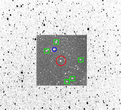
Figure 1: Oskar-Lühning telescope (dark background) and Planet Transit Search Telescope (light background) field of views. Qatar-1 is indicated with a large red circle centered on the OLT field of view, along with the comparison stars as green squares. The small blue circle upward and to right of Qatar-1 indicates the reference star used to produce the differential photometry.

3 Data analysis

3.1 Data preparation

IRAF provides heliocentric corrections, therefore our time stamps are given as heliocentric Julian dates ($\mathrm{HJD}_{\mathrm{UTC}}$) and are converted into barycentric Julian dates ($\mathrm{BJD}_{\mathrm{TDB}}$) using the web tool provided by Eastman et al. (2010).

3.2 Fit approach

We fitted the transit data with the transit model developed by Mandel & Agol (2002), making use of their occultquad FORTRAN routine. From the transit light curve, we can directly infer the following parameters: the orbital period $P$, the mid-transit time $T_{0}$, the radius ratio $p=R_{p}/R_{s}$, the semi-major axis (in stellar radii) $a/R_{s}$, and the orbital inclination $i$. For our fits we assumed a quadratic limb-darkening law with fixed coefficients $u_{1}$ and $u_{2}$.

3.3 Limb-darkening coefficients

Alsubai et al. (2011) presented a spectroscopic characterization of Qatar-1 based on comparing their observed spectrum with synthetic template spectra and suggested that Qatar-1 has an effective temperature $T_{\mathrm{eff}}$ of $4861\pm 125$ K, a surface gravity $\log{g}$ of $4.536\pm 0.024$, and solar metallicity [Fe/H] of $0.20\pm 0.10$. Because our observations with OLT and PTST were obtained using different (non-standard) filter sets, we decided to calculate angle-resolved synthetic spectra from spherical atmosphere models using PHOENIX (Hauschildt & Baron (1999), Witte et al. (2009)) for a star with effective temperature $T_{\mathrm{eff}}=4900$ K, [Fe/H] = 0.20 and $\log{g}=4.5$, thereby closely matching the spectroscopic parameters of Qatar-1A. We then convolved each synthetic spectrum with the OLT and PTST filter transmission functions and integrated in the wavelength domain to compute intensities as a function of $\mu=\cos{\theta}$, where $\theta$ is the angle between the line of sight and the radius vector from the center of the star to a reference position on the stellar surface. The thus derived intensities were then fitted with a quadratic limb-darkening prescription, viz.

$$I(\mu)/I(1)=1-u_{1}(1-\mu)-u_{2}(1-\mu)^{2}\ ,$$

to obtain the $u_{1}$ and $u_{2}$ limb-darkening coefficients. As an aside, we note that the best approach to obtain limb-darkening coefficients would be to fit a more sophisticated bi-parametric approximation to the stellar intensities (Claret & Hauschildt, 2003) to the PHOENIX intensities, which produces the smallest deviations in the generation of the limb-darkening coefficients, which fits the stellar limb better. However, to introduce such a limb-darkening law in the production of primary transit light curves would be computationally cumbersome. Moreover, Qatar-1 is a nearly grazing system, where changes in limb darkening do not strongly affect the primary transit light curves. We checked that the time that the planet spends in the small-$\mu$ regime is very short. Furthermore, at a given time the planet covers a broad range of $\mu$-values. Neglecting these points in determining the limb-darkening coefficients will probably not affect the subsequent parameter determination. To calculate the OLT and PTST limb-darkening coefficients, we fitted a quadratic limb-darkening law to PHOENIX intensities, neglecting the data points between $\mu$ = 0 and $\mu$ = 0.1. Fig. 2 shows the OLT and PTST limb-darkening normalized functions, and Table 2 the fitted limb-darkening coefficients.

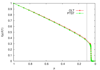
Figure 2: Qatar-1 normalized intensities considering the OLT and PTST filter transmission functions. Data points on the right of the vertical dashed line were not considered in the fitting procedure.

Table 2: Best-fit limb-darkening coefficients (LDCs) for OLT and PTST, along with the 1 $\sigma$ errors.

LDCs	OLT	PTST
$u_{1}$	0.5860 $\pm$ 0.0053	0.6025 $\pm$ 0.0051
$u_{2}$	0.1170 $\pm$ 0.0075	0.1140 $\pm$ 0.0073

3.4 Parameter errors

To determine reliable errors for the fit parameters given the mutual dependence of the model parameters, we explored the parameter space by sampling from the posterior-probability distribution using a Markov-chain Monte-Carlo (MCMC) approach.

The near-grazing transit geometry of Qatar-1 introduces a substantial amount of correlation between the system parameters, which can easily render the MCMC sampling process inefficient. To cope with these difficulties we used a modification to the usually employed Metropolis-Hastings sampling algorithm, which is able to adapt to the strong correlation structure. This modified Metropolis-Hastings algorithm is described in the seminal work by Haario et al. (2001) and has become known as the adaptive Metropolis (AM) algorithm. It works like the regular Metropolis-Hastings sampler, but relies on the idea of allowing the proposal distribution to depend on the previous values of the chain.

The regular Metropolis-Hastings algorithm produces chains based on a proposal distribution that may depend on the current state of the chain. The proposal distribution is often chosen to be a multivariate normal distribution with fixed covariance. The main difference between the regular Metropolis sampler and AM is that AM updates the covariance matrix during the sampling, e.g. every 1000 iterations. Because the proposal distribution is thus tuned based on the entire sampling run, AM chains in fact lose the Markov property. Nonetheless, it can be shown that the algorithm retains the correct ergodic properties under very general assumptions, i.e., the covariance matrix stabilizes during the sampling process and AM chains properly simulate the target distribution (Haario et al., 2001; Vihola, 2011). Although adaptive MCMC algorithms are a recent development, they have successfully been used by other authors in the astronomical community, for instance by Balan & Lahav (2009); Irwin et al. (2010) and Irwin et al. (2011).

Our MCMC calculations make extensive use of routines of PyAstronomy, a collection of Python routines providing a convenient interface for fitting and sampling algorithms implemented in the PyMC (Patil et al., 2010) and SciPy (Jones et al., 2001) packages. The AM sampler is implemented in the PyMC package, which is publicly available for download. We refer to the detailed online documentation.

We checked that AM does yield correct results for simulated data sets with parameters close to Qatar-1, and found that this approach showed fast convergence and was efficient. To express our lack of more a priori knowledge regarding the Qatar-1 system parameters, we assumed uninformative uniform prior probability distributions for all parameters, but we found that the parameters are well determined, so that the actual choice of the prior is unimportant for our results.

*

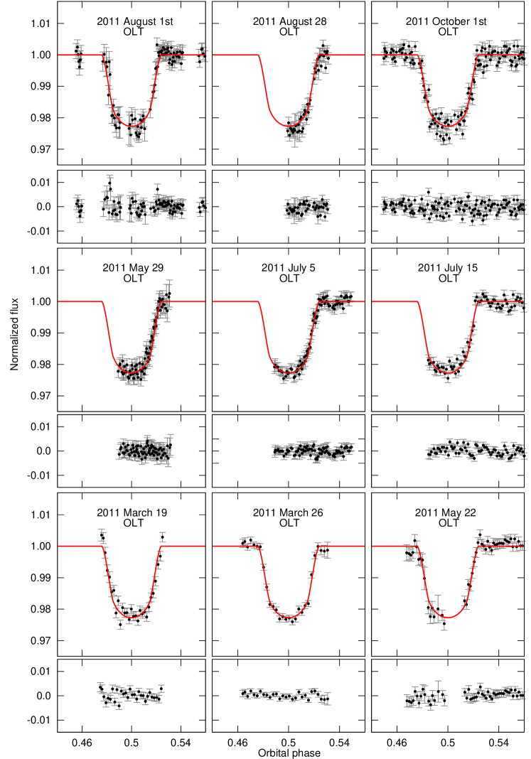
Figure 3: OLT and PTST light curves (top panels). Superposed is the Mandel & Agol (2002) primary transit light-curve model in a continuous line, considering the parameters obtained in Section 3.2. As indicated by the dates, the light curves evolve in time from bottom to top and from left to right. The residuals (bottom panels) have been calculated after subtracting the best transit fit parameters.

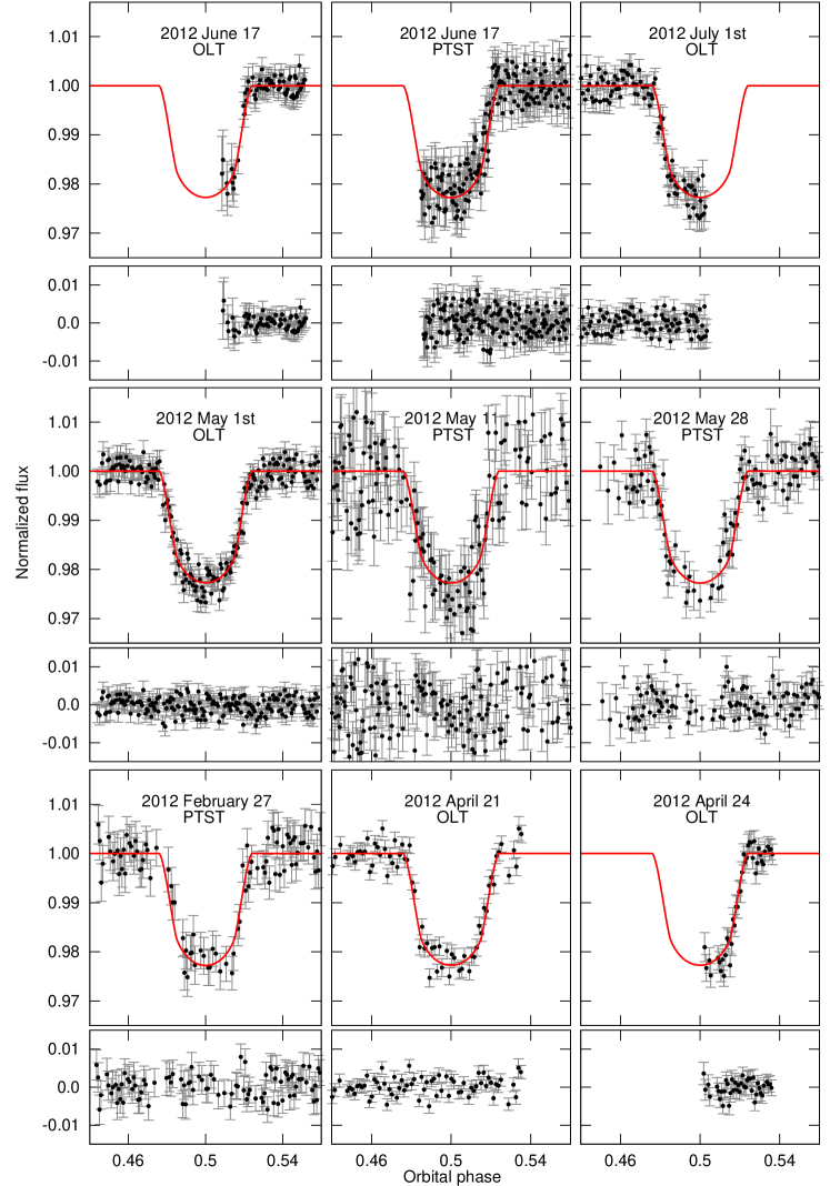
Figure 4: Same as Figure 3

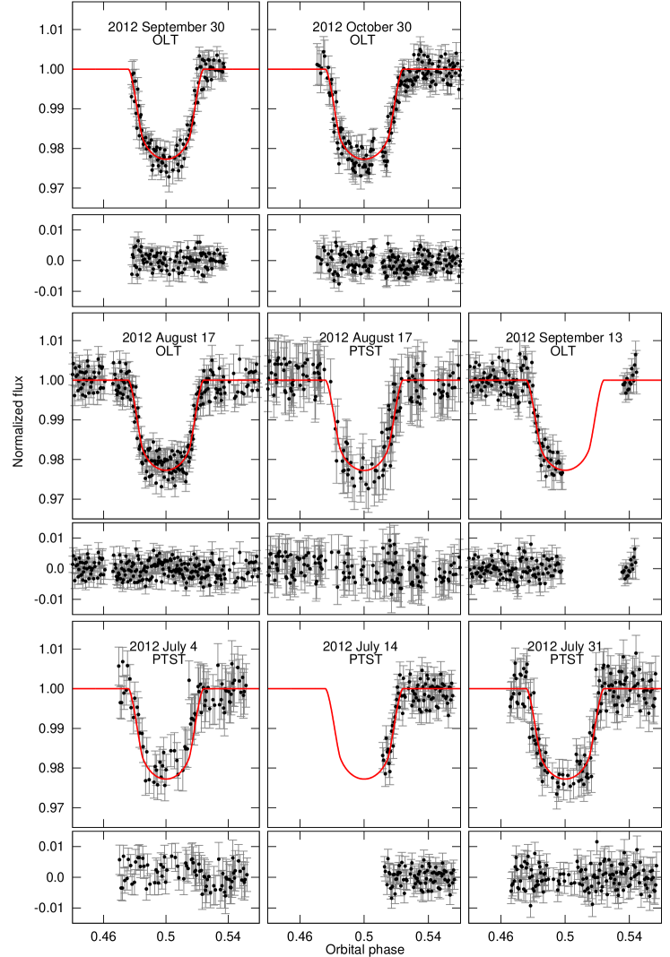
Figure 5: Same as Figure 3

In Figure 3 we show our 26 obtained light curves, along with the residuals after removing the primary transit feature. Our final relative photometry is available in its entirety in machine-readable form in the electronic version of this paper. First columns contain $\mathrm{BJD}_{\mathrm{TDB}}$, second columns normalized flux, and third columns individual errors.

3.5 Correlated noise

Carter & Winn (2009) (and references therein) studied how time-correlated noise affects the estimation of the parameter of transiting systems. To quantify whether and to what extent our light curves are affected by red noise, we reproduced part of their analysis as follows: First, we produced residuals from our final fits by subtracting the primary transit model from each light curve. We individually divided each light curve into M bins of equal duration. Since our data are not always equally spaced, we calculated a mean value N of data points per bin. If the data are not affected by red noise, they should follow the expectation of independent random numbers,

$$\sigma_{N}=\sigma_{1}N^{-1/2}[M/(M-1)]^{1/2}\ ,$$

where $\sigma_{1}$ is the sample variance of the unbinned data and $\sigma_{N}$ is the sample variance (or RMS) of the binned data, with the following expression:

$$\sigma_{N}=\sqrt{\frac{1}{M}\sum_{i=1}^{M}(<\hat{\mu_{i}}>-\hat{\mu_{i}})^{2}}\ ,$$

where $\hat{\mu_{i}}$ is the mean value of the residuals per bin, and $<\hat{\mu_{i}}>$ is the mean value of the means.

If correlated noise is present, then each value $\sigma_{N}$ will differ by a factor $\beta_{N}$ from their expectation. The parameter $\beta$, an estimation of the strength of correlated noise in the data, is found by averaging $\beta_{N}$ over a range $\Delta n$ corresponding to time scales that are judged to be most important. For data sets free of correlated noise, we expect $\beta$ = 1. For primary transit observations, $\Delta n$ is the duration of ingress or egress. For Qatar-1, the time between first and second contact (or equivalently, the time between third and fourth contact) is $\sim$ 15 minutes.

In Figure 6 we show the results of our correlated noise analysis for nine of the longest light curves. Black lines represent the expected behavior in the absence of red noise, and red and green lines represent the variance of the binned data for OLT and PTST, respectively, as a function of bin size. As expected, the larger the bin size, the smaller the RMS. For each light curve we calculated $\beta$ considering $\Delta n$ = 15 minutes. For the OLT and PTST primary transits, $\beta$ lies between $\beta$ = 0.78 and $\beta$ = 1.33, with $<\beta>$ = 1.038. Thus, there is no evidence for significant correlated noise in our light curves.

Finally, Pont et al. (2006) suggested to enlarge individual photometric errors by a factor $\beta$ to account for systematic effects on the light curves. This would increase the parameter errors without changing the parameter estimates. Since our light curves do not present any strong evidence of correlated noise, we did not modify the individually derived errors.

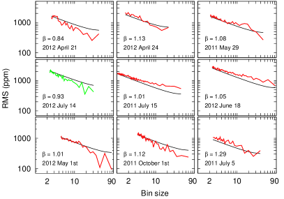
Figure 6: Qatar-1 RMS in parts per Million (ppm) of the time-binned residuals as a function of bin size in logarithmic scale. Red and green lines correspond to OLT and PTST data respectively, and black lines show the expected behavior under the presence of uncorrelated noise.

3.6 Effects of exposure times and transit coverage

The accuracy in determining of the mid-transit time is affected by the number of data points during transit and the number of off-transit data points, even more so when a normalization is involved.

To study whether the mid-transits are affected by the transit observation duration, we computed the timing residual magnitudes as a function of the number of data points per transit. If any systematic effect dominates the light curves, a larger timing offset for those transits that are sampled the least is expected. We show our results in Figure 7. Since the light curves are normalized and the mid-transits might be sensitive to normalizations, we also computed the timing-residual magnitudes as a function of the number of off-transit data points. We used the Pearson correlation coefficient $r$ to quantify the correlation of the mid-transit offsets. In both cases this was $r\sim$ -0.11 for all data points, and $r\sim$ 0.05, which rules out the 0^th epoch, which was expected to be zero by construction. We found no significant correlation.

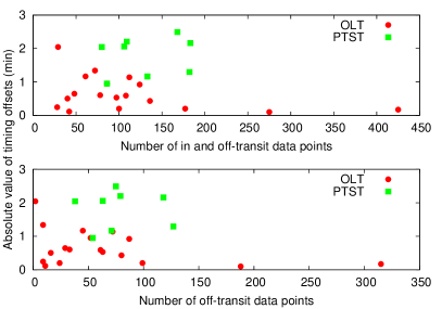
Figure 7: Timing-residual magnitudes in minutes as a function of in and off-transit data point number (top) and off-transit data point number only (bottom). The outermost point close to zero is the primary transit, which was selected to be the $0^{th}$ epoch. Mid-transit errors are not plotted to avoid visual contamination.

Kipping (2010) studied the effects of finite integration times on the determination of the orbital parameters. He showed that the time difference between the mid-transit moment and the nearest light curve data point might cause a shift in the TTV signal, which is expected to be one half of the rate sampling. To test how significant this effect is over our light curves, we calculated the mean exposure times per observing night, which was about 80 seconds. Figure 8 shows the mean exposure times per night, versus the magnitude of the timing residuals. Most of the data points lying around the half-mean exposure time ($\sim$ 35 seconds) were identified to have the most accurate mid-transit timings, with exposure times of about one minute, which makes it unlikely that they are affected by a sampling effect. The Pearson correlation coefficient of $r$ = -0.15 again reveals no significant correlation.

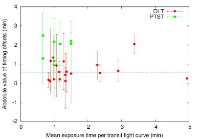
Figure 8: Timing-residual magnitudes in minutes for OLT (red circles) and PTST (green squares), as a function of mean exposure times. The horizontal dashed line indicates half of the mean exposure time.

3.7 Results

In general terms, the parameters $P$ and $T_{0}$ are usually correlated with each other, but are uncorrelated with the remaining transit parameters. Therefore, these parameters can be determined quite accurately without interference of the remaining ones. We used a Nelder-Mead simplex to approach the best-fit solution, which is provided as the starting values of the MCMC sampler. The AM algorithm then samples from the posterior distribution for the parameters to obtain error estimates. After $10^{8}$ iterations we discarded a suitable burn-in (typically $10^{6}$ samples) and determined the combination of parameters resulting in the lowest deviance. We consider the lowest deviance as our global best-fit solution. The errors were derived from the 68 % highest probability density or credibility intervals (1 $\sigma$). Our results are summarized in Table 3. None of our fit parameters are consistent with those reported by Alsubai et al. (2011); a possible explanation for this inconsistency might be that these authors determined the system parameters using only four light curves, two of which were incomplete, obtained in less than two weeks. During the revision of this paper, Covino et al. (2013) presented high-precision radial velocity measurements from which the Rossiter-McLauglin effect was observed. The authors also obtained five new photometric transit light curves, from which the orbital parameters of the system were improved. With respect to the orbital period, one of the most important parameters for determining TTVs, our best-fitted orbital period seems to be consistent within errors with the one found by Covino et al. (2013).

Table 3: Best-fit (lowest deviance) parameters for our 26 transits of Qatar-1 after $10^{8}$ MCMC samples. LDCs are fixed at the values reported in Table 2.

Parameter	Value (1$\sigma$ errors)	Alsubai et al. (2011)
$i$ (∘)	84.52 $\pm$ 0.24	83.47${}^{+0.40}_{-0.36}$
$p$ ($R_{p}/R_{s}$)	0.1435 $\pm$ 0.0008	0.1454 $\pm$ 0.0015
$a$ ($R_{s}$)	6.42 $\pm$ 0.10	6.1005${}^{+0.067}_{-0.065}$
$P$ (days)	1.4200246 $\pm$ 0.0000004	1.420033 $\pm$ 0.000016

To obtain individual mid-transit times $T_{mid,i}$, we considered the best-fit values of $p$, $a$, $i$, $u_{1}$, $u_{2}$, and $P$. We specified Gaussian priors on these parameters and refitted each one of the 26 individual transit light curves for the mid-transit time $T_{mid,i}$. Our results are listed in Tab. 4 together with the derived 1 $\sigma$ errors on these transit times. To compute the timing deviations compared with a constant period we fitted the observed mid-transit times $T_{o,i}$ to the expression

$$T_{o,i}=P\cdot E_{i}+T_{o}\ ,$$

finding the ephemeris

$$P=1.4200246\pm 0.0000004\leavevmode\nobreak\ \mbox{days}$$

$$T_{0}=2456157.42204\pm 0.0001\leavevmode\nobreak\ \mbox{\mbox{$\mathrm{BJD}_{\mathrm{TDB}}$}}$$

as best-fitting values. All errors are obtained from the 68.27% confidence level of the marginalized posterior distribution for the parameters. With these parameters we computed the OC-values also listed in Tab. 4. We used the available simultaneous observations separated two months from each other as a diagnostics of our fitting procedure. Both mid-transits (epochs -43 and 0) are consistent with each other within the errors.

4 Transit timing variation analysis

4.1 OC diagram

In the absence of any timing variations we expect no significant deviations of the derived OC-values from zero. Testing the null hypothesis OC = 0 with a $\chi^{2}$-test, we found ${\chi}^{2}_{red}$ = 2.56 with 24 degrees of freedom. This high value led us to reject the null hypothesis that OC vanishes.

We then applied the Lomb-Scargle periodogram (Lomb (1976), Scargle (1982), Zechmeister & Kürster (2009)) to search for any significant periodicity contained in the OC diagram. Figure 9 shows the data points used to perform the periodogram, along with a list in Table 4. The resulting periodogram reveals a first peak at $\nu_{TTV,1}$ = 0.00759 $\pm$ 0.00075 cycl P^-1 (corresponding to a period of 187 $\pm$ 17 days) and a second one at about half the frequency $\nu_{TTV,2}$ = 0.00367 $\pm$ 0.00059 cycl P^-1 (corresponding to 386 $\pm$ 54 days). For both periodic signals, new ephemeris were refitted using the linear trend and a sinusoidal variation in the form

$$T_{o,i}=P\cdot E_{i}+T_{o}+A_{TTV}\sin(2\pi\nu_{TTV}[E_{i}-E_{TTV}]).$$

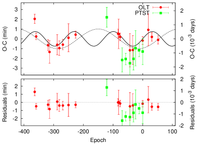
Figure 9: OC diagram for Qatar-1 in minutes (left axis) and days (right axis) considering the OLT (red circles) and PTST (green squares) data points, along with the timing residuals. Our initial best-fitting model is overplotted with a continuous black line, and the second one with a dashed black line.

Table 4: OLT (top) and PTST (bottom) fitted mid-transits with 1 $\sigma$ errors and the OC data points.

Epoch	$T_{0}$	O-C
	$\mathrm{BJD}_{\mathrm{TDB}}$- 2455500	(days)
OLT
-364	140.53449 $\pm$ 0.00033	0.00142
-359	147.63337 $\pm$ 0.00023	0.00017
-319	204.43373 $\pm$ 0.00038	-0.00045
-314	211.53337 $\pm$ 0.00079	-0.00093
-288	248.45453 $\pm$ 0.00071	-0.00042
-281	258.39446 $\pm$ 0.00051	-0.00066
-269	275.43500 $\pm$ 0.00037	-0.00041
-250	302.41596 $\pm$ 0.00099	0.00007
-226	336.49677 $\pm$ 0.00026	0.00030
-83	539.56037 $\pm$ 0.00031	0.00037
-81	542.40039 $\pm$ 0.00104	0.00035
-76	549.50031 $\pm$ 0.00027	0.00014
-43	596.36017 $\pm$ 0.00119	-0.00081
-33	610.56044 $\pm$ 0.00102	-0.00079
0	657.42192 $\pm$ 0.00027	-0.00012
19	684.40315 $\pm$ 0.00113	0.00064
31	701.44294 $\pm$ 0.00031	0.00014
52	731.26325 $\pm$ 0.00029	-0.00007
PTST
-121	485.60059 $\pm$ 0.00070	0.00153
-69	559.43884 $\pm$ 0.00086	-0.00150
-57	576.47921 $\pm$ 0.00040	-0.00143
-43	596.35925 $\pm$ 0.00084	-0.00173
-31	613.39986 $\pm$ 0.00078	-0.00142
-24	623.34079 $\pm$ 0.00125	-0.00066
-12	640.38093 $\pm$ 0.00045	-0.00081
0	657.42114 $\pm$ 0.00093	-0.00090

For the most significant frequency, the fitted amplitude and phase are $A_{TTV,1}$ = 0.00052 $\pm$ 0.0002 days (equivalently, 0.75$\pm$ 0.28 minutes) and $\phi_{TTV,1}$ = 0.04 $\pm$ 0.05. We then recalculated $\chi^{2}_{red}$ = 1.85 for the first frequency. Using an F-test to check the significance of the fit improvement we obtained a p-value of 0.02, indicating that the sinusoidal trend does indeed provide a better description than the constant at 2.8$\sigma$ level. We can also compare the models using the Bayesian information criterion, BIC = $\chi^{2}$ + k ln N, which penalizes the number k of model parameters given N = 26 data points. We obtained BICs of 68.1 and 57.2 for the constant and sinusoidal trend, respectively. Since the BIC is no more than a criterion for model selection among a set of models, the method one more time favors the sinusoidal trend.

We finally estimated the false-alarm probability (FAP) of the TTV signal, using a bootstrap resampling method by randomly permuting the mid-transit values ($5\times 10^{5}$ times) along with their individual errors, fixing the observing epochs and calculating the Lomb-Scargle periodogram afterward. We estimated the FAP as the frequency with which the highest power in the scrambled periodogram exceeds the maximal power in the original periodogram. In this fashion we estimated an FAP of 0.05% for our observed TTV signal, consistent with our previous estimates.

To further check whether the addition of the sinusoidal variation provides an explanation for the timing offsets, we made use of the mid-transits of Qatar-1 available in the Exoplanet Transit Database (ETD) (Poddaný et al., 2010) to reinforce our results. The ETD data are very heterogeneous, we therefore converted the best 26 mid-transits from $\mathrm{HJD}_{\mathrm{UTC}}$ to $\mathrm{BJD}_{\mathrm{TDB}}$. Each ETD primary transits has a data quality indicator ranging from 1 (small scatter and good time-sampling) to 4 (the opposite). For our analysis we only selected the transits with quality flags 1 (5 primary transits) and 2 (21 primary transits). These transits span a total of $\sim$ 500 epochs. We produced the OC diagram (Table 5) using the following fitted ephemeris:

$$P=1.4200223\pm 0.0000004\leavevmode\nobreak\ \mbox{days}$$

$$T_{0}=2455518.410961\pm 0.0002\leavevmode\nobreak\ \mbox{\mbox{$\mathrm{BJD}_{\mathrm{TDB}}$}}.$$

Table 5: ETD-fitted instant of minima with 1 $\sigma$ errors and the OC data points.

Epoch	$T_{0}$	O-C
	$\mathrm{BJD}_{\mathrm{TDB}}$- 2455500	(days)
ETD
0	18.41096 $\pm$ 0.00020	0
93	150.47263 $\pm$ 0.00058	-0.00040
119	187.39490 $\pm$ 0.00063	0.00128
155	238.51887 $\pm$ 0.00062	0.00445
158	242.77532 $\pm$ 0.00088	0.00083
189	286.79573 $\pm$ 0.00059	0.00055
194	293.89601 $\pm$ 0.00041	0.00072
196	296.73493 $\pm$ 0.00039	-0.00040
219	329.39461 $\pm$ 0.00049	-0.00123
231	346.43651 $\pm$ 0.00054	0.00039
238	356.37502 $\pm$ 0.00077	-0.00124
246	367.73872 $\pm$ 0.00054	0.00227
264	393.29753 $\pm$ 0.00051	0.00068
265	394.71796 $\pm$ 0.00049	0.00109
329	485.59892 $\pm$ 0.00067	0.00062
341	502.63734 $\pm$ 0.00044	-0.00122
401	587.84221 $\pm$ 0.00053	0.00230
412	603.46031 $\pm$ 0.00058	0.00016
419	613.40040 $\pm$ 0.00038	0.00009
434	634.70330 $\pm$ 0.00038	0.00266
443	647.47797 $\pm$ 0.00041	-0.00286
446	651.74233 $\pm$ 0.00046	0.00142
450	657.41961 $\pm$ 0.00049	-0.0013
455	664.52112 $\pm$ 0.00043	0.00001
495	721.32109 $\pm$ 0.00073	-0.00090
510	742.62146 $\pm$ 0.00048	-0.0008

The primary transit selected for the 0^th epoch is the most accurate one of all available light curves. We produced a periodogram using the resulting timing offsets and found one peak at $\nu_{TTV,ETD}$ = 0.00784 $\pm$ 0.0011 cycl P^-1 (corresponding to a period of 181 $\pm$ 22 days) with an amplitude of $A_{TTV,ETD}$ = 0.0009 $\pm$ 0.0005 days (equivalently, 1.29 $\pm$ 0.72 minutes) and a phase of $\phi_{TTV,ETD}$ = 0.02 $\pm$ 0.03. Within the errors, the frequency, amplitude, and phase are consistent with the ones found using OLT and PTST data. Figure 10 shows two periodograms, the one on top produced using our data, and the one on bottom produced with ETD data.

Figure 10: Zechmeister & Kürster (2009) periodograms generated from the timing residuals of Qatar-1, showing a peak at $\nu_{TTV,1}$ = 0.00759 $\pm$ 0.00075 cycl P^-1 (our data, top panel) and $\nu_{TTV,ETD}$ = 0.0078 $\pm$ 0.0011 cycl P^-1 (ETD data, bottom panel). Vertical lines indicate the 1$\sigma$ error on $\nu_{TTV,1}$. The parameters derived from our periodogram are maximum power = 6.1, and FAP for the maximum-power peak = 0.19%.

4.2 Error analysis

To test the reliability of our error estimates for each mid-transit time and to check the influence of the error magnitude on the estimated peak frequencies, we iteratively constructed new Lomb-Scargle periodograms randomly increasing the individual mid-transit errors mostly by a factor of two.

At each iteration, we first added the absolute value of a random number that was drawn from a normal distribution ($\mu$ = 0, $\sigma$ = 0.0004 days) to each mid-transit error, and calculated the leading frequency afterward. After $5\times 10^{5}$ of such iterations, we found that the only effect on the error increment is the permutation of the leading frequency from $\nu_{TTV,1}$ to $\nu_{TTV,2}$. This permutation occurred only $\sim$9% of the times.

In Figure 11 we show the resulting histogram of the calculated leading frequencies. They all fall inside the 1$\sigma$ errors of $\nu_{TTV,1}$ and $\nu_{TTV,2}$, estimated from our original fits. Thus, the derived mid-transit errors do not significantly affect the outcome in terms of dominating frequencies.

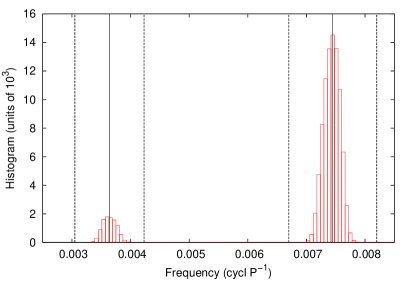
Figure 11: Histogram of the leading frequencies obtained after incrementing the individual mid-transit errors, in units of $10^{3}$. Vertical continuous lines indicate our best two leading frequencies $\nu_{TTV,1}$ and $\nu_{TTV,2}$, along with 1$\sigma$ errors (dashed vertical lines).

5 Interpretation of the observed transit timing variations

For the purposes of this section we assumed that the reported TTVs are real and explored possible physical scenarios that would explain the observed variations. We considered both the $\sim$190 and $\sim$380 day periods, although the ETD data set is consistent only with the former period. As is well known, a suitably placed third body in the Qatar-1 system can lead to perturbations in the orbit of Qatar-1b, which manifest themselves as TTVs. Since there are no complete analytical solutions to the three-body problem, we made use of a numerical integration scheme. Because a planetary orbit is determined by a large number of parameters (i.e., the eccentricity, the longitude of the nodes, the orbital inclination, among many others), it is a real challenge to estimate true orbital parameters by fitting TTV models to ground-based mid-transit shifts only. We therefore started with the simplest approach and assumed coplanar orbits using the inclination derived from the light curve fitting, along with the best-fit orbital period, and the transiting planet mass and eccentricity obtained by Alsubai et al. (2011) as fixed. Given trial mass, orbital period, eccentricity, longitude of periastron and ascending node, and the time of periastron passage, the n-body code calculates the time of occurrence of the primary transits taking into account the interaction between the planets. We specifically considered two scenarios, a putative low-mass planet in a resonant orbit relative close to Qatar-1b, and a putative high-mass planet or brown dwarf in an 190-day orbit around Qatar-1.

5.1 Weak perturber in resonance with Qatar-1b

Two planetary bodies in orbital resonance with each other will experience long-term changes in their orbital parameters. On one hand, since only a relative short stretch of data (less than two years) is available, expecting a unique solution is too ambitious. On the other hand, most of the perturber’s dynamical setups will translate into negligible TTVs.

Taking into account these difficulties, we calculated the modeled TTV scatter for a two-planetary system, to study in advance which would be the parameter space giving rise to TTVs similar to the scatter of our data. We first considered both bodies in circular orbits and then the perturber in an eccentric orbit. The mass of the perturber was systematically changed between 1, 8, and 15 $M_{\oplus}$. Figure 12 shows our results. The vertical dashed lines indicate the 2:1, 3:1, and 5:2 resonances. In these regions, perturbers of the order of several Earth masses would produce TTVs similar to the observed ones.

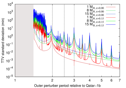
Figure 12: Simulated TTV standard deviation in minutes of Qatar-1b as a function of the outer perturber period, for two values of eccentricity and three values of perturber masses. The gray area on the left correspond to perturber orbits that would make the Qatar-1b orbit unstable. The mean motion resonances 2:1, 3:1, and 5:2 are indicated with vertical dashed lines.

We thus investigated some possible solutions that would satisfy the first two TTV periods assuming the specific resonant orbits indicated in Figure 12. As an example we show in Fig. 13 and Tab. 6 three arbitrary cases; similar solutions can be derived with other choices of resonant orbits. To produce Fig. 13 we ran our n-body simulation with specified initial conditions (cf., Tab. 6) and compared the results with the observed OC-values and our (original) sinusoidal fit (cf., Fig. 13). As is clear from Fig. 13, all these solutions have $\chi^{2}$ values similar to our first fitting attempt. Thus, it is futile to produce a proper fitting procedure.

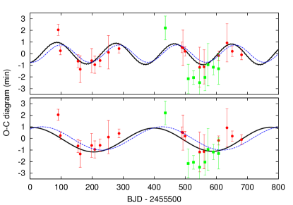
Figure 13: OC diagram for OLT (red circles) and PTST (green squares) data points plus n-body solutions for two different dynamical scenarios (black lines) and our best initial sinusoidal fit (blue dashed lines) artificially shifted in phase for a better comparison.

Table 6: Three possible solutions for our two main TTV signals for three different dynamical scenarios. From top to bottom, resonances are 5:2, 2:1, and 3:1.

Resonance 5:2, $\sim$190 days	Qatar-1b	Perturber
Mass ($M_{Jup}$)	1.090	0.019
Orbital period (days)	1.4200246	3.550061
Eccentricity	0	0.3
$\omega$ (∘)	274	21
$\Omega$ (∘)	235	90
$t$	0	0
Resonance 2:1, $\sim$190 days	Qatar-1b	Perturber
Mass ($M_{Jup}$)	1.090	0.005
Orbital period (days)	1.4200246	2.8400492
Eccentricity	0	0.15
$\omega$ (∘)	190	30
$\Omega$ (∘)	330	120
$t$	0	0
Resonance 3:1, $\sim$380 days	Qatar-1b	Perturber
Mass ($M_{Jup}$)	1.090	0.035
Orbital period (days)	1.4200246	4.2600738
Eccentricity	0	0.135
$\omega$ (∘)	202	31
$\Omega$ (∘)	300	90
$t$	0	0

5.2 Massive perturber in a 190-day orbit

As an alternative to a lower-mass perturber in a resonant orbit, we also considered a more massive perturber in a non-resonant 190-day orbit. In this case the TTV amplitude strongly depends on the mass and the eccentricity of the assumed perturber. Again considering the simplest case of coplanar orbits and both longitude of periastron and longitude of the ascending node fixed to zero, we computed the amplitude of the TTV signal as a function of the perturber mass and its orbital eccentricity using our n-body code, and we compared the predicted TTV amplitudes with those observed. Our results are shown in Fig. 14, where we plot the expected TTV amplitude as a function of the perturber mass for various eccentricities in the range between zero and 0.8. For low eccentricity values we require perturber masses of more than 80 Jupiter masses, i.e., we would require a low-mass star. For eccentricities above 0.6 a brown dwarf could explain the observed TTV amplitudes. It is obvious that such an object would lead to RV variations in the host of Qatar-1, which could in principle be observed. Since for a very eccentric orbit the RV variations are concentrated around the periastron passage and since only ten days of RV measurements are available for Qatar-1 so far, any long-term RV variations of Qatar-1 are unknown so far and could confirm or reject the presence of a massive perturber.

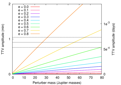
Figure 14: TTV amplitude as a function of the mass of the perturber for different eccentricity values. The black continuous line shows the best-fitted amplitude to our OC diagram, along with 1$\sigma$ errors (dashed lines).

6 Conclusions

Our analysis of the mid-timing residuals of Qatar-1 taken during almost two years indicate that the orbital period of the exoplanet is not constant. The observed long-term timing variations are highly significant from a statistical point of view and can be explained by very different physical scenarios. RV monitoring of Qatar-1 will provide an upper limit to the mass of a possible perturber and continued timing observations of Qatar-1 are required to better delineate the solution space for the possible perturber geometries.