DCPT-13/31
The Sakai-Sugimoto soliton

Abstract

The Sakai-Sugimoto model is the preeminent example of a string theory description of holographic QCD, in which baryons correspond to topological solitons in the bulk. Here we investigate the validity of various approximations of the Sakai-Sugimoto soliton that are used widely to study the properties of holographic baryons. These approximations include the flat space self-dual instanton, a linear expansion in terms of eigenfunctions in the holographic direction and an asymptotic power series at large radius. These different approaches have produced contradictory results in the literature regarding properties of the baryon, such as relations for the electromagnetic form factors. Here we determine the regions of validity of these various approximations and show how to relate different approximations in contiguous regions of applicability. This analysis clarifies the source of the contradictory results in the literature and resolves some outstanding issues, including the use of the flat space self-dual instanton, the detailed properties of the asymptotic soliton tail, and the role of the UV cutoff introduced in previous investigations. A consequence of our analysis is the discovery of a new large scale, that grows logarithmically with the ’t Hooft coupling, at which the soliton fields enter a nonlinear regime. Finally, we provide the first numerical computation of the Sakai-Sugimoto soliton and demonstrate that the numerical results support our analysis.

1 Introduction

There are still some unresolved puzzles regarding aspects of bulk solitons in holographic models of QCD. These include the validity of the flat space self-dual instanton used in the Sakai-Sugimoto model and the large distance behaviour of the electromagnetic form factors of the baryon. In this paper we shall address these issues and provide analytic resolutions that are confirmed by numerical investigations.

The cornerstone of all models of baryons in holographic QCD is that solitons in the bulk correspond to Skyrmions on the boundary. This correspondence was first observed by Atiyah and Manton [1] in four-dimensional Euclidean space, where the bulk soliton is the self-dual Yang-Mills instanton. The correspondence can be formulated as a flat space version of holography [2]. Holographic QCD differs from the Atiyah-Manton approach in that spacetime is curved with AdS-like behaviour and a five-dimensional Chern-Simon term is included that generates an abelian electric charge for the soliton. Here AdS-like means that the curvature is negative and there is a conformal boundary. The combination of the curvature of spacetime and the electromagnetic repulsion provides a stability that fixes the size of the soliton. These features are common to all models of holographic QCD, whether bottom-up or top-down.

Top-down approaches are derived from a string embedding and the Sakai-Sugimoto model [3, 4] is the prototypical example for top-down AdS/QCD models. In these models, the validity of the supergravity approximation requires working with a large number of colours $N_{c}$ and a large value of the ’t Hooft coupling $\lambda$. Although $N_{c}$ is just an overall multiplicative factor in the action, and thus irrelevant at the classical level, $\lambda$ plays a vital role for the classical soliton, as it controls the ratio between the Yang-Mills and Chern-Simons terms. In particular, for large $\lambda$ the size of the soliton becomes parametrically small with respect to the curvature scale. This suggests that most of the energy density of the soliton is concentrated in a small region of space, where the effect of the curvature has little influence on the fields of the soliton. This motivates the approach used in [5, 6], where the soliton is approximated by the flat space self-dual Yang-Mills instanton, with a size determined by minimization of the energy function on the instanton moduli space that results by restricting the full energy functional to the space of self-dual instanton fields. Note that this approximation is based on the assumption that the curvature and Chern-Simons term do not significantly alter the soliton fields, even though they are crucial in determining its size. We shall put this assumption to the test by numerically computing the Sakai-Sugimoto soliton and comparing it to the self-dual instanton. Furthermore, we show how to improve the self-dual instanton approximation via a simple generalization that maintains the $SO(4)$ symmetry of the instanton but introduces a more general profile function.

The soliton properties at large distance, and consequently the baryon electromagnetic form factors of the dual theory, have been calculated by expanding the self-dual instanton tail at the linear level and then extending this linear solution into the curved space at large distance from the core [7, 8, 9]. This approach relies on the fact that, for a small soliton, there is a region from the soliton core to the curvature scale in which the soliton is essentially in a linear regime and the curvature effects remain negligible. The result of this linear analysis is that the baryon density, and consequently all the electromagnetic form factors (including those of exited baryons obtained from a zero mode quantization) are exponentially suppressed at large distance. This is in contrast to the situation for other models, including the standard Skyrme model with massless pions, where the baryon density has an algebraic decay.

Bottom-up approaches are equally good toy-models for AdS/QCD, as long as they incorporate the features of confinement and chiral symmetry breaking. These models are relieved of the requirement of a string theory embedding, so there is a free choice of any AdS-like metric (provided it has a conformal boundary in the UV) and $\lambda$ need not be small. The Pomarol-Wulzer model [10] is an example in this category, where the metric is a slice of AdS₅ with a finite IR boundary at which left and right gauge fields are subject to matching conditions that mimic the salient features of the Sakai-Sugimoto model. Numerical computations of the Pomarol-Wulzer soliton have been performed at a value of the coupling that is of order one (where the soliton size is comparable to the curvature scale of the AdS₅ slice), together with an asymptotic power series at large radius [11]. These results show that the baryon form factors have an algebraic decay, as in the Skyrme model, and not an exponential decay.

Cherman, Cohen and Nielsen [12] have described model independent relations for the baryon form factors at large distance. These relations are satisfied by the baryon form factors computed in the Skyrme model and the Pomarol-Wulzer model but not by those of the Sakai-Sugimoto model obtained from the linear analysis. The exponential decay of the soliton fields in the Sakai-Sugimoto model lies at the heart of this failure. Later, Cherman and Ishii [13] adapted the large radius expansion in [11] to the Sakai-Sugimoto model and found that the form factors have an algebraic decay and indeed satisfy the model independent relations, contradicting the earlier result of the linear analysis. However, their approach required the introduction of a UV cutoff and problems arise in attempting to remove this cutoff, so it is not clear which of the conflicting results is correct. Very recently, a preprint has appeared in which the large radius expansion has been applied to a general metric [14] and a conclusion drawn regarding the UV cutoff introduced into the Sakai-Sugimoto model. We shall comment on this conclusion in section 4.7, where we derive the correct procedure for removing the UV cutoff.

The contradictory conclusions described above raise a number of issues and questions concerning the use and validity of the various approximations and approaches. In fact, several candidates have been suggested for the source of the disagreement. One possibility is that the use of the flat space self-dual instanton in the Sakai-Sugimoto model is at the root of the problem. The validity of this approximation has never been tested, either numerically or analytically, and one may worry about a mechanism that allows the curvature and Chern-Simons term to stabilize the instanton size without altering the form of its fields. We shall test the use of the instanton approximation, firstly by introducing a generalization that allows some deformation of the instanton fields, and secondly via direct numerical computation of the Sakai-Sugimoto soliton. Our results strongly support the validity of the self-dual instanton approximation for large ’t Hooft coupling.

Another possibility is that either the linear expansion in [7] or the large radius expansion in [13] are not valid in the Sakai-Sugimoto model. In fact, we shall show that both approaches are valid but they are applicable in different regions of space. The contradictory results concerning the soliton tail, and consequently the baryon form factors, is a result of applying the linear expansion in an inappropriate region. The resolution of all the discrepancies in the literature resides in the existence of a new scale. This is a large scale that grows logarithmically with the ’t Hooft coupling and is therefore much larger than both the radius of curvature and the size of the small instanton. The linear expansion should be thought of as an expansion in $\lambda^{-1}$, where the first term solves the linearised field equations. However, higher order terms are larger than the first order term both at the small instanton scale, which is of order $\lambda^{-{1}/{2}},$ and crucially at the new large scale of order $\log{\lambda}$. The fundamental property of the system is that there is a transition from a linear to a nonlinear regime at large distance. The existence of this new large scale explains the discrepancy over the form factor computations, which depend on the fall-off of the soliton tail. The vital observation is that the large $\lambda$ and large radius limits do not commute. The crucial terms with algebraic decay are suppressed by additional powers of $\lambda^{-1}$ in comparison to the terms with exponential decay, so the algebraic decay is only evident at the large scale of order $\log{\lambda}$.

The outline of this paper is as follows. In section 2 we review the main aspects of the Sakai-Sugimoto model. In section 3 we discuss the flat space self-dual instanton approximation and our radial generalization. Section 4 is devoted to the calculation of the tail properties of the soliton, and in particular a determination of the regions of validity of alternative approximations. By comparing these different approximations we are able to relate them to each other and hence predict the emergence of the new large scale. A numerical computation of the Sakai-Sugimoto soliton is described in section 5, where the numerical results are shown to support our analytic findings. Finally, some concluding remarks are made in section 6.

2 The Sakai-Sugimoto model

Consider a five-dimensional spacetime with a warped metric of the form

$$ds^{2}=H(z)\,dx_{\mu}dx^{\mu}+\frac{1}{H(z)}dz^{2}.$$ (2.1)

Here $x_{\mu},$ with $\mu=0,1,2,3,$ are the coordinates of four-dimensional Minkowski spacetime and $z$ is the spatial coordinate in the additional holographic direction. The signature is $(-,+,+,+,+)$.

A class of spacetimes that are particularly relevant for holographic baryons corresponds to the choice

$$H=\left(1+\frac{z^{2}}{L^{2}}\right)^{p},$$ (2.2)

where $L$ and $p$ are positive constants, with the former setting a curvature length scale. In this paper we focus on the Sakai-Sugimoto model [3, 4], which corresponds to the choice $p=\frac{2}{3}$. For general $p$ the scalar curvature of the metric, after setting the length scale $L=1$, is

$$R=-4H^{-3/4}\left(H^{3/4}H^{\prime}\right)^{\prime}=-\frac{4p\left(2+(7p-2)z^{2}\right)}{\left(1+z^{2}\right)^{2-p}}.$$ (2.3)

This formula shows that the value of $p$ is crucial in determining the qualitative features of the spacetime. For $p\leq 1$ the curvature is finite as $z\to\infty.$ For $p=1$ the spacetime is asymptotically AdS₅ with constant negative curvature $-20$. For $p>\frac{2}{7}$ the curvature is negative for all $z$ and for $p>\frac{1}{2}$ the theory has a conformal boundary. In the case of a conformal boundary it is often useful to introduce conformal coordinates

$$ds^{2}=H(z(u))\left(dx_{\mu}dx^{\mu}+du^{2}\right),$$ (2.4)

where $u$ solves the equation $du/dz=1/H(z).$ For large $z$ the asymptotic behaviour is $u(z)\simeq c_{1}+c_{2}/z^{2p-1},$ for some constants $c_{1}$ and $c_{2}.$ Thus $u\to c_{1}$ as $z\to\infty$, revealing the conformal boundary.

Given the above properties, we refer to the metric as AdS-like if $p\in(\frac{1}{2},1],$ since there is then a conformal boundary and the curvature is negative and finite. The Sakai-Sugimoto model is a generic example with $p=\frac{2}{3}.$ Unless otherwise specified, from now on we will fix the values $L=1$ and $p=\frac{2}{3},$ though occasionally we will reintroduce these constants to indicate the more general dependence.

The Sakai-Sugimoto model is a $U(2)$ gauge theory in the five-dimensional spacetime introduced above. Our index notation is that uppercase indices include the holographic direction whilst lowercase indices exclude this additional dimension. Furthermore, greek indices include the time coordinate whilst latin indices (excluding $z$) run over the spatial coordinates. Thus, for example,

$$\Gamma,\Delta,\ldots=0,1,2,3,z,\quad\mu,\nu,\ldots=0,1,2,3,\quad I,J,\ldots=1,2,3,z,\quad i,j,\ldots=1,2,3.$$ (2.5)

To fix conventions, the gauge potential ${\cal A}_{\Gamma}$ is hermitian and under a gauge transformation, $G\in U(2),$ it transforms as ${\cal A}_{\Gamma}\mapsto G{\cal A}_{\Gamma}G^{-1}+i(\partial_{\Gamma}G)G^{-1}.$ The associated field strength is ${\cal F}_{\Gamma\Delta}=\partial_{\Gamma}{\cal A}_{\Delta}-\partial_{\Delta}{\cal A}_{\Gamma}+i[{\cal A}_{\Gamma},{\cal A}_{\Delta}]$ and the covariant derivative is $D_{\Gamma}\heartsuit=\partial_{\Gamma}\heartsuit+i[A_{\Gamma},\heartsuit].$ The action is the sum of a Yang-Mills term and a $U(2)$ Chern-Simons term

$${\cal S}=-\frac{N_{c}\lambda}{216\pi^{3}}\int\sqrt{-g}\ \frac{1}{2}{\rm tr}\left({\cal F}_{\Gamma\Delta}{\cal F}^{\Gamma\Delta}\right)\,d^{4}x\,dz+\frac{N_{c}}{24\pi^{2}}\int\ \omega_{5}({\cal A})\,d^{4}x\,dz,$$ (2.6)

where $g$ is the earlier warped metric with $p=\frac{2}{3}.$ The factors $N_{c}$ and $\lambda$ are respectively the number of colours and the ’t Hooft coupling of the dual theory. Note that the number of colours acts just as a multiplicative factor and therefore plays a trivial role in the classical physics in the bulk. In particular, by keeping $\lambda$ fixed and taking the limit $N_{c}\to\infty$ we can always make any quantum corrections negligible.

Decomposing the $U(2)$ gauge potential into a sum of non-abelian $SU(2)$ and abelian $U(1)$ components

$${\cal A}_{\Gamma}=A_{\Gamma}+\frac{1}{2}\widehat{A}_{\Gamma},\qquad\qquad{\cal F}_{\Gamma}=F_{\Gamma}+\frac{1}{2}\widehat{F}_{\Gamma},$$ (2.7)

the $U(2)$ Chern-Simons term, up to a total derivative, is

$$\frac{N_{c}}{24\pi^{2}}\int\left(\frac{3}{8}\widehat{A}_{\Gamma}{\rm tr}\,({F}_{\Delta\Sigma}{F}_{\Xi\Upsilon})+\frac{1}{16}\widehat{A}_{\Gamma}\,\widehat{F}_{\Delta\Sigma}\widehat{F}_{\Xi\Upsilon}\right)\varepsilon^{\Gamma\Delta\Sigma\Xi\Upsilon}\,d^{4}x\,dz.$$ (2.8)

The action, conveniently rescaled, becomes

$$S = \frac{216\pi^{3}}{N_{c}\lambda}{\cal S}$$ (2.9)

$$= \int\left\{-\frac{1}{4H^{1/2}}{\widehat{F}}_{\mu\nu}{\widehat{F}}^{\mu\nu}-\frac{H^{3/2}}{2}{\widehat{F}}_{\mu z}{\widehat{F}}^{\mu z}\right.\left.-\frac{1}{2H^{1/2}}{\rm tr}\left({F}_{\mu\nu}{F}^{\mu\nu}\right)-H^{3/2}{\rm tr}\left({F}_{\mu z}{F}^{\mu z}\right)\right\}\,d^{4}x\,dz$$

$$+\frac{1}{\Lambda}\int\left(\widehat{A}_{\Gamma}{\rm tr}\,({F}_{\Delta\Sigma}{F}_{\Xi\Upsilon})+\frac{1}{6}\widehat{A}_{\Gamma}\,\widehat{F}_{\Delta\Sigma}\widehat{F}_{\Xi\Upsilon}\right)\,\varepsilon^{\Gamma\Delta\Sigma\Xi\Upsilon}\,d^{4}x\,dz,$$

where the indices are now raised using the flat 5-dimensional Minkowski metric tensor $\eta_{\Gamma\Delta}$. For convenience, in the above we have introduced the rescaled ’t Hooft coupling

$$\Lambda=\frac{8\lambda}{27\pi}.$$ (2.10)

As we are concerned with the static soliton solution of the theory, from now on we shall restrict to the case of time independent fields. The appropriate static ansatz is

$${A}_{0}=0,\qquad A_{I}={A}_{I}(x_{J}),\qquad\widehat{A}_{0}=\widehat{A}_{0}(x_{J}),\qquad\widehat{A}_{I}=0,$$ (2.11)

so that the abelian potential generates an electric field $\widehat{F}_{I0}=\partial_{I}\widehat{A}_{0}$. The action restricted to static fields is then

$$S = \int\left\{\frac{1}{2H^{1/2}}(\partial_{i}\widehat{A}_{0})^{2}+\frac{H^{3/2}}{2}(\partial_{z}\widehat{A}_{0})^{2}\right.\left.-\frac{1}{2H^{1/2}}{\rm tr}\left({F}_{ij}^{2}\right)-H^{3/2}{\rm tr}\left({F}_{iz}^{2}\right)\right\}\,d^{4}x\,dz$$ (2.12)

$$+\frac{1}{\Lambda}\int\widehat{A}_{0}\ {\rm tr}\,({F}_{IJ}{F}_{KL})\,\varepsilon_{IJKL}\,d^{4}x\,dz.$$

The static field equations that follow from the variation of this action are

$$\frac{1}{H^{1/2}}D_{j}F_{ji}+D_{z}(H^{3/2}F_{zi})=\frac{1}{\Lambda}\varepsilon_{iJKL}F_{KL}\partial_{J}\widehat{A}_{0}$$ (2.13)

$$H^{3/2}D_{j}F_{jz}=\frac{1}{\Lambda}\varepsilon_{ijk}F_{jk}\partial_{i}\widehat{A}_{0}$$ (2.14)

$$\frac{1}{H^{1/2}}\partial_{i}\partial_{i}\widehat{A}_{0}+\partial_{z}(H^{3/2}\partial_{z}\widehat{A}_{0})=\frac{1}{\Lambda}{\rm tr}\,(F_{IJ}F_{KL})\,\varepsilon_{IJKL}.$$ (2.15)

Baryon number is identified with the $SU(2)$ instanton number of the soliton

$$B=-\frac{1}{32\pi^{2}}\int{\rm tr}(F_{IJ}F_{KL})\,\varepsilon_{IJKL}\,d^{3}x\,dz,$$ (2.16)

and the Chern-Simons coupling implies that the instanton charge density sources the abelian electric field.

For later computational purposes, it will be convenient to rewrite the action by rearranging the terms as

$$S = \int\left\{\frac{H^{3/2}}{2}\bigg{(}(\partial_{I}\widehat{A}_{0})^{2}-{\rm tr}\left({F}_{IJ}^{2}\right)\bigg{)}+\frac{1-H^{2}}{2H^{1/2}}\bigg{(}(\partial_{i}\widehat{A}_{0})^{2}-{\rm tr}\left({F}_{ij}^{2}\right)\bigg{)}\right\}\,d^{4}x\,dz,$$ (2.17)

$$+\frac{1}{\Lambda}\int\widehat{A}_{0}\ {\rm tr}\,({F}_{IJ}{F}_{KL})\,\varepsilon_{IJKL}\,d^{4}x\,dz.$$

3 Radial and self-dual approximations

As we shall see, the static soliton solution of the field equations that follow from (2.12) is quite complicated. Even for the single static soliton, symmetry reduction can only reduce the field equations to coupled partial differential equations for five functions of two variables, which then need to be solved numerically. This approach will be described in detail in section 5, where we present the results of the first numerical computation of the Sakai-Sugimoto soliton.

The lack of an exact solution has motivated various approximate descriptions of the soliton, some of which we shall discuss later. First we consider a new approximation, in which the fields are assumed to have $SO(4)$ spherical symmetry. Because of the warp factor in the metric, such an assumption is clearly incompatible with the true solution of the field equations, so no exact solutions can be obtained in this way. However, we can certainly restrict the functional space to such a set of symmetric trial fields and determine the fields that are stationary points of the restricted action. The advantage of this approach is that it reduces the problem to a single ordinary differential equation, which is much easier to deal with than the full coupled partial differential equations. Furthermore, the radial approximation is a generalization of the self-dual flat space instanton approximation that has been used heavily in previous studies, so we are able to further investigate this approximation by examining how the radial approximation compares to the self-dual approximation in the large $\Lambda$ limit. The obvious disadvantage of the radial approximation is that it is unclear whether the approximate fields provide a reasonable description of the true solution. Fortunately, our later numerical solution will allows us to investigate this aspect too.

To specify the fields within the radial approximation we define the coordinates $\rho\geq 0$ and $\theta\in[0,\pi]$ by

$$\rho=\sqrt{x_{1}^{2}+x_{2}^{2}+x_{3}^{2}+z^{2}},\qquad z=\rho\cos{\theta}.$$ (3.1)

The radial approximation involves two real profile functions $a(\rho)$ and $b(\rho)$ and is given by

$$\widehat{A}_{0}=a(\rho),\qquad\qquad A_{I}=-{\sigma}_{IJ}x_{J}\,b(\rho),$$ (3.2)

where $\sigma_{IJ}$ is the anti-symmetric ’t Hooft tensor defined in terms of the Paul matrices $\sigma_{i}$ by

$$\sigma_{ij}=\varepsilon_{ijk}\sigma_{k},\qquad\sigma_{zi}=\sigma_{i}.$$ (3.3)

The non-abelian field has the same $SO(4)$ symmetry as the self-dual instanton, but has a more general radial profile function.

The instanton charge density is

$$-\frac{1}{32\pi^{2}}{\rm tr}(F_{IJ}F_{KL})\,\varepsilon_{IJKL} = \frac{3}{\pi^{2}}b(1-\rho^{2}b)(2b+\rho b^{\prime})$$ (3.4)

$$= \frac{1}{\pi^{2}\rho^{3}}\left(\frac{3}{2}(\rho^{2}b)^{2}-(\rho^{2}b)^{3}\right)^{\prime}$$

yielding the instanton number

$$B=c^{2}(3-2c),\quad\mbox{where}\quad c=\lim_{\rho\to\infty}(\rho^{2}b).$$ (3.5)

The requirement that $B=1$ therefore determines that $c=1,$ giving the large $\rho$ behaviour

$$b=\frac{1}{\rho^{2}}+{\cal O}\bigg{(}\frac{1}{\rho^{4}}\bigg{)}.$$ (3.6)

In evaluating the action density of the radial field, the first term to consider is

$${\rm tr}\left({F}_{IJ}^{2}\right)=12(2b+\rho b^{\prime})^{2}+48b^{2}(1-b\rho^{2})^{2}.$$ (3.7)

The remaining term that is required is

$${\rm tr}\left({F}_{ij}^{2}\right)=\frac{8}{\rho}\bigg{(}6\rho b^{2}+2b^{3}\rho(\rho^{2}+2z^{2})(b\rho^{2}-2)+b^{\prime}(b^{\prime}\rho+4b)(\rho^{2}-z^{2})\bigg{)}.$$ (3.8)

Substituting these expressions into the action (2.17), writing $z=\rho\cos\theta$ and performing the angular integration over $\theta$ gives

$$\frac{S}{2\pi^{2}} = \int\Big{\{}(P_{1}-P_{2}+P_{3})a^{\prime 2}-12P_{1}\big{(}(2b+\rho b^{\prime})^{2}+4b^{2}(1-b\rho^{2})^{2}\big{)}$$ (3.9)

$$+8\big{(}6b^{2}P_{2}+2b^{3}\rho^{2}(P_{2}+2P_{3})(b\rho^{2}-2)+b^{\prime}(b^{\prime}\rho+4b)\rho(P_{2}-P_{3})\big{)}\Big{\}}\rho^{3}\,d\rho\,dt$$

$$-\frac{16}{\Lambda}\int a\left(3(\rho^{2}b)^{2}-2(\rho^{2}b)^{3}\right)^{\prime}\,d\rho\,dt,$$

where the three functions $P_{1,2,3}(\rho)$ are defined by the following angular integrals

$$P_{1}(\rho) = \frac{1}{\pi}\int_{0}^{\pi}H(\rho\cos{\theta})^{3/2}\,\sin^{2}\theta\,d\theta=\frac{1}{2}+\frac{1}{8}\rho^{2}$$

$$P_{2}(\rho) = \frac{1}{\pi}\int_{0}^{\pi}\frac{H(\rho\cos{\theta})^{2}-1}{H(\rho\cos{\theta})^{1/2}}\,\sin^{2}\theta\,d\theta=\frac{1}{6}\rho^{2}-\frac{1}{72}\rho^{4}+{\cal O}(\rho^{6})$$

$$P_{3}(\rho) = \frac{1}{\pi}\int_{0}^{\pi}\frac{H(\rho\cos{\theta})^{2}-1}{H(\rho\cos{\theta})^{1/2}}\,\sin^{2}\theta\,\cos^{2}\theta\,d\theta=\frac{1}{12}\rho^{2}-\frac{5}{576}\rho^{4}+{\cal O}(\rho^{6}).$$ (3.10)

The field equation for $a(\rho)$, that follows from the variation of (3.9), may be integrated once to yield

$$a^{\prime}=-\frac{8\rho b^{2}(3-2\rho^{2}b)}{\Lambda(P_{1}-P_{2}+P_{3})},$$ (3.11)

where the constant of integration has been set to zero in order to have a vanishing electric field at the origin $a^{\prime}(0)=0$. Integration by parts of the Chern-Simons term in (3.9), together with the solution (3.11), produces the following energy functional, that depends only on the profile function $b(\rho),$

$$\frac{E}{2\pi^{2}} = \int\Big{\{}\frac{64\rho^{2}b^{4}(3-2\rho^{2}b)^{2}}{\Lambda^{2}(P_{1}-P_{2}+P_{3})}+12P_{1}\big{(}(2b+\rho b^{\prime})^{2}+4b^{2}(1-b\rho^{2})^{2}\big{)}$$

$$-8\big{(}6b^{2}P_{2}+2b^{3}\rho^{2}(P_{2}+2P_{3})(b\rho^{2}-2)+b^{\prime}(b^{\prime}\rho+4b)\rho(P_{2}-P_{3})\big{)}\Big{\}}\rho^{3}\,d\rho.$$

Minimization of this energy gives a second order ordinary differential equation for $b(\rho)$ that must be solved subject to the boundary conditions

$$b^{\prime}(0)=0\quad\mbox{and}\quad\rho^{2}b\to 1\quad\mbox{as}\quad\rho\to\infty.$$ (3.13)

Given this profile function, $a(\rho)$ can be obtained by integrating (3.11). We shall present this numerical solution at the end of this section, but first we see how the flat space self-dual instanton approximation fits within this formalism.

In the case of large ’t Hooft coupling (which is required in top-down approaches) the Chern-Simons term is parametrically suppressed with respect to the Yang-Mills term. The role of the Chern-Simons coupling is to provide an electric contribution that stabilize the soliton against the shrinking induced by the spacetime curvature. Large $\Lambda$ should therefore correspond to a small soliton size, so that space is approximately flat in the soliton core. This motivates the use of the flat space self-dual instanton to approximate the soliton [5, 6].

To investigate the large $\Lambda$ limit it is useful to first introduce the rescaled coordinate $\widetilde{\rho}=\sqrt{\Lambda}\rho.$ The boundary condition $\rho^{2}b\to 1$ as $\rho\to\infty,$ determines that the appropriate associated rescaling of the profile function is $\widetilde{b}=b/\Lambda.$ In terms of these variables the energy (3) can be written as $E=\sum_{j=0}^{\infty}E_{j}\Lambda^{-j},$ where the first two terms are

$$E_{0}=12\pi^{2}\int\Big{\{}\big{(}(2\widetilde{b}+\widetilde{\rho}\widetilde{b}^{\prime})^{2}+4\widetilde{b}^{2}(1-\widetilde{b}\widetilde{\rho}^{2})^{2}\big{)}\Big{\}}\widetilde{\rho}^{3}\,d\widetilde{\rho},$$ (3.14)

$$E_{1}=\frac{\pi^{2}}{3}\int\Big{\{}4\widetilde{b}^{2}\big{(}192\widetilde{b}^{2}(2\widetilde{\rho}^{2}\widetilde{b}-3)^{2}+\widetilde{\rho}^{4}\widetilde{b}^{2}-2\widetilde{\rho}^{2}\widetilde{b}+6\big{)}+5\widetilde{\rho}\widetilde{b}^{\prime}(\widetilde{\rho}\widetilde{b}^{\prime}+4b)\Big{\}}\widetilde{\rho}^{5}\,d\widetilde{\rho}.$$ (3.15)

Restricting to the leading order term, the energy $E_{0}$ is minimized by the profile function of the flat space self-dual instanton

$$\widetilde{b}=\frac{1}{\widetilde{\rho}^{2}+\widetilde{\mu}^{2}},$$ (3.16)

where $\widetilde{\mu}$ is the rescaled arbitrary size of the instanton. The leading order term in the energy is $E_{0}=8\pi^{2}$ and is independent of the size of the instanton.

The self-dual approximation involves restricting the profile function to the self-dual form (3.16) and using the next order term in the energy, $E_{1},$ as an energy function on the moduli space of instanton sizes. Explicitly, substituting (3.16) into (3.15) and performing the integration yields

$$E_{1}=2\pi^{2}\bigg{(}\frac{2}{3}\widetilde{\mu}^{2}+\frac{256}{5\widetilde{\mu}^{2}}\bigg{)},$$ (3.17)

which is minimized when

$$\widetilde{\mu}={4}\bigg{(}\frac{3}{10}\bigg{)}^{1/4}.$$ (3.18)

Returning to unscaled variables, with $\mu=\widetilde{\mu}/\sqrt{\Lambda}$ the size of the instanton, the self-dual approximation gives

$$E=2\pi^{2}\bigg{(}4+\frac{2}{3}\mu^{2}+\frac{256}{5\Lambda^{2}\mu^{2}}\bigg{)}+{\cal O}\bigg{(}\frac{1}{\Lambda^{2}}\bigg{)},$$ (3.19)

where

$$\mu=\frac{4}{\sqrt{\Lambda}}\bigg{(}\frac{3}{10}\bigg{)}^{1/4}.$$ (3.20)

A similar scaling analysis of equation (3.11) shows that the leading order result for $a^{\prime}$ simply corresponds to replacing the term $P_{1}-P_{2}+P_{3}$ in (3.11) by its flat space limit $\frac{1}{2}.$ After substituting the self-dual approximation $b=1/(\rho^{2}+\mu^{2})$ and integrating, the result is

$$a=\frac{8(\rho^{2}+2\mu^{2})}{\Lambda(\rho^{2}+\mu^{2})^{2}}.$$ (3.21)

Note that $a(0)={16}/({\Lambda\mu^{2}})=\sqrt{\frac{10}{3}}$ is independent of $\Lambda$ within this self-dual approximation.

In summary, the first term in the energy (3.19) is independent of the instanton size and is simply the flat space self-dual Yang-Mills result of $8\pi^{2}$ in our units. The second term is ${\cal O}(\mu^{2})$ and also derives from the Yang-Mills functional but from the leading order correction to the the metric expansion around flat space. This gravitational contribution drives the instanton towards zero size. The third term is ${\cal O}(1/\mu^{2})$ and is the first contribution from the electrostatic abelian field. This term resists the shrinking of the instanton size. These competing effects combine to produce the finite size (3.20), which is small for large $\Lambda,$ with the energy dominated by the flat space self-dual contribution. The correction from the size stabilizing terms is subleading and is ${\cal O}(1/\Lambda)$.

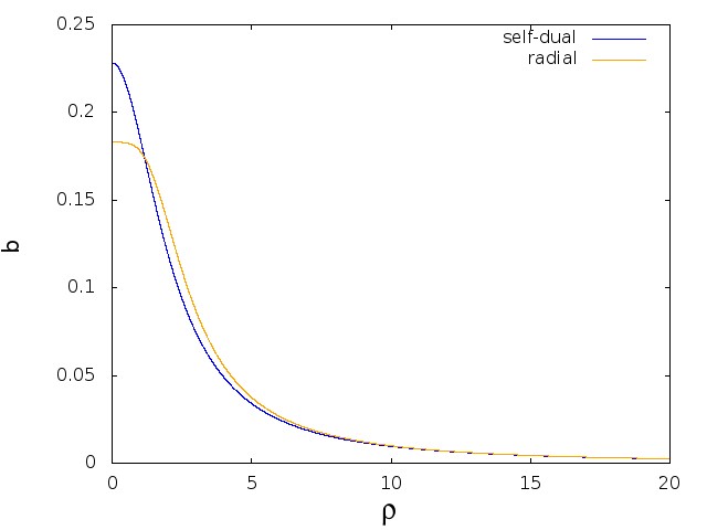
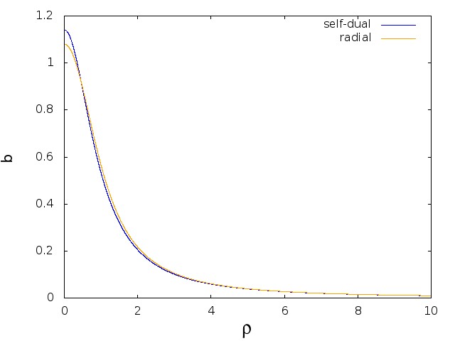
Figure 1: The profile function $b(\rho)$ using the flat space self-dual approximation (blue curve) and the radial approximation (orange curve). The left and right images correspond to the coupling $\Lambda=2$ and $\Lambda=10$ respectively.

Returning to the radial approximation, the profile function $b(\rho)$ that minimizes the energy (3) subject to the boundary conditions (3.13), was obtained using a shooting method with a fourth order Runge-Kutta algorithm to solve the second order ordinary differential equation obtained from the variation of the energy. The results are displayed in Figure 1 for two values of the coupling $\Lambda=2,10.$ These plots illustrate the flow of the radial approximation to the self-dual approximation as $\Lambda\to\infty.$ For finite $\Lambda$ the main difference between the radial and self-dual approximations is that the self-dual approximation overestimates the value at the origin. As we shall see later, the full numerical solution confirms this overestimation, with the radial approximation being an improvement that reduces, but does not eliminate, this error.

The above rescaling to the self-dual instanton in the $\Lambda\to\infty$ limit is a radial restriction of the following rescaling used in [5, 6]

$$\widetilde{x}^{I}=\sqrt{\Lambda}{x}^{I},\qquad\widetilde{t}=t,\qquad\widetilde{A}_{I}=A_{I}/\sqrt{\Lambda},\qquad\widetilde{\widehat{A}}_{0}=\widehat{A}_{0}.$$ (3.22)

Defining $\widetilde{H}=H(\widetilde{z}/\sqrt{\Lambda}),$ then in the rescaled variables the action becomes

$${S} = \int\left\{-\frac{\widetilde{H}^{3/2}}{2}{\rm tr}\left(\widetilde{F}_{IJ}^{2}\right)-\frac{1-\widetilde{H}^{2}}{2\widetilde{H}^{1/2}}{\rm tr}\left({\widetilde{F}}_{ij}^{2}\right)\right.$$ (3.23)

$$\qquad\qquad\ +\left.\frac{1}{\Lambda}\left(\frac{\widetilde{H}^{3/2}}{2}(\widetilde{\partial}_{I}\widetilde{\widehat{A}}_{0})^{2}+\frac{1-\widetilde{H}^{2}}{2\widetilde{H}^{1/2}}(\widetilde{\partial}_{i}\widetilde{\widehat{A}}_{0})^{2}\right)\right\}\,d^{4}\widetilde{x}\,d\widetilde{z}$$

$$+\frac{1}{\Lambda}\int\ \widetilde{\widehat{A}}_{0}\ {\rm tr}\,(\widetilde{F}_{IJ}\widetilde{F}_{KL})\,\varepsilon_{IJKL}\,d^{4}\widetilde{x}\,d\widetilde{z}.$$

Using the metric (2.2), with a general value of $p,$ and expanding in $1/\Lambda$ gives

$$S=\int\bigg{\{} -\frac{1}{2}{\rm tr}\left(\widetilde{F}_{IJ}^{2}\right)$$ (3.24)

$$+\frac{1}{\Lambda}\left(-\frac{3}{4}p\widetilde{z}^{2}{\rm tr}\left(\widetilde{F}_{IJ}^{2}\right)+p\widetilde{z}^{2}{\rm tr}\left(\widetilde{F}_{ij}^{2}\right)+\frac{1}{2}(\widetilde{\partial}_{I}\widetilde{\widehat{A}}_{0})^{2}+\widetilde{\widehat{A}}_{0}\ {\rm tr}\,(\widetilde{F}_{IJ}\widetilde{F}_{KL})\,\varepsilon_{IJKL}\right)$$

$$+{\cal O}\left(\frac{1}{\Lambda^{2}}\right)\qquad\bigg{\}}\,d^{4}\widetilde{x}\,d\widetilde{z},$$

which highlights the convenience of the rescaling (3.22). The leading order term is scale invariant and is simply the Yang-Mills action in flat space. The next term is of order $1/\Lambda$ and contains the size stabilizing contributions from both the abelian field and the curvature (due to the positive value of $p$). The action of the leading order term is minimized by the self-dual instanton and the term of order $1/\Lambda$ defines an action on the self-dual instanton moduli space that fixes the size of the instanton.

In summary, the way to extract the self-dual instanton limit is to convert to the rescaled coordinates (3.22) and then perform the $\Lambda\to\infty$ limit

$$\lim_{\Lambda\to\infty}\widetilde{{\cal A}}(\widetilde{x})=\widetilde{{\cal A}}_{self-dual}(\widetilde{x}),$$ (3.25)

to converge to a self-dual instanton with a size $\widetilde{\mu}$ in rescaled coordinates given by(3.18). For large but finite $\Lambda$ the small unscaled instanton size is $\mu=\widetilde{\mu}/\sqrt{\Lambda}.$

It is important to note that the self-dual limit has nothing to say about the asymptotic fields of the soliton at large distance. This is because the rescaling performed in (3.22) involves zooming in to a scale of order $1/\sqrt{\Lambda}$. To study the fields of the soliton at distances greater than $1/\sqrt{\Lambda}$ requires alternative approaches that we describe in the next section.

4 The soliton tail

4.1 A linear expansion in flat space

In this subsection we consider a linear expansion that we shall see is valid in the region ${L}/{\sqrt{\Lambda}}\lesssim\rho\lesssim L,$ where we recall that we have set $L=1.$ This region is far enough from the soliton core that a linear expansion is possible but is close enough to the origin that the curvature of the metric can be neglected by setting $H=1.$

To derive this expansion we still use $1/\Lambda$ as the small parameter of the expansion, but now we keep the length scale fixed rather than zooming in to the core. In this limit

$$\lim_{\Lambda\to\infty}\Lambda\,{\cal A}(x)={\cal A}_{tail}(x),$$ (4.1)

where ${\cal A}_{tail}$ is a finite term that solves the linearised field equations. The task is to compute ${\cal A}_{tail}(x)$ and to confirm its region of applicability.

We define the $1/\Lambda$ expansion

$$A_{I}=A^{(1)}_{I}+A^{(2)}_{I}+\dots,\qquad\qquad\widehat{A}_{0}=\widehat{A}_{0}^{(1)}+\widehat{A}_{0}^{(2)}+\dots$$ (4.2)

in which

$$A_{I}^{(n)},\,\widehat{A}_{0}^{(n)}\propto\frac{1}{\Lambda^{n}}.$$ (4.3)

The limit (4.1) picks up only the first term in this expansion

$${\cal A}_{tail}(x)=\Lambda\,{\cal A}^{(1)}(x).$$ (4.4)

As the space is now taken to be flat, the calculation in this subsection will involve expanding the self-dual instanton to provide the leading order contribution. This result will then be used in the next subsection to match to a linear analysis in curved space.

To perform the analysis it is convenient to write the self-dual instanton in the gauge in which it has the ’t Hooft form

$$A_{I}=\frac{1}{2}{\sigma}_{IJ}\partial_{J}\log{\left(1+\frac{\mu^{2}}{\rho^{2}}\right)}.$$ (4.5)

Given that $\mu^{2}={\cal O}(1/\Lambda)$ then the first term in the expansion is

$$A^{(1)}_{I}=-{\sigma}_{IJ}\frac{x_{J}\,\mu^{2}}{\rho^{4}}=\frac{\mu^{2}}{2}{\sigma}_{IJ}\partial_{J}\frac{1}{\rho^{2}}\propto\frac{1}{\Lambda},$$ (4.6)

which satisfies the field equations ((2.13) and (2.14) with $H=1$) at the linear level since

$$\partial_{I}A^{(1)}_{I}=0\qquad\mbox{and}\qquad\partial_{J}\partial_{J}A^{(1)}_{I}=0.$$ (4.7)

These equations are simply those of an abelian gauge potential: the first is the condition of Coulomb gauge and the second is the vanishing of the Laplacian.

The term $A^{(1)}_{I}$ gives the dominant contribution to the field strength

$$F_{IJ}^{(1)} = \partial_{I}A^{(1)}_{J}-\partial_{J}A^{(1)}_{I}=\frac{2\mu^{2}}{\rho^{4}}\left({\sigma}_{IJ}+\frac{2}{\rho^{2}}({\sigma}_{JK}{x}_{K}{x}_{I}-{\sigma}_{IK}{x}_{K}{x}_{J})\right).$$ (4.8)

From (3.21) the abelian gauge potential at linear order is

$$\widehat{A}_{0}^{(1)}=\frac{8}{\Lambda\rho^{2}},$$ (4.9)

which satisfies the final field equation ((2.15) with $H=1$) at linear order.

Defining $F_{IJ}^{(2)}=\partial_{I}A^{(2)}_{J}-\partial_{J}A^{(2)}_{I},$ at second order the field equations are

$$\partial_{I}{F}^{(2)}_{IJ}+i[A_{I}^{(1)},{F}^{(1)}_{IJ}]=0\qquad\mbox{and}\qquad\partial_{I}\partial_{I}\widehat{A}_{0}^{(2)}=0,$$ (4.10)

with solution

$$A^{(2)}_{I}={\sigma}_{IJ}\frac{x_{J}\,\mu^{4}}{\rho^{6}}\propto\frac{1}{\Lambda^{2}},\qquad\qquad\widehat{A}_{0}^{(2)}=0.$$ (4.11)

The next non-zero term in $\widehat{A}_{0}$ is at third order, where the field equation gives

$$\partial_{I}\partial_{I}\widehat{A}_{0}^{(3)}=\frac{1}{\Lambda}{\rm tr}\,({F}^{(1)}_{IJ}{F}^{(1)}_{KL})\,\varepsilon_{IJKL},$$ (4.12)

and is solved by

$$\widehat{A}_{0}^{(3)}=-\frac{8\mu^{4}}{\Lambda\rho^{6}}\propto\frac{1}{\Lambda^{3}}.$$ (4.13)

For this expansion to be reliable requires $||A^{(1)}_{I}||\lesssim||A^{(2)}_{I}||$ and $||\widehat{A}_{0}^{(1)}||\lesssim||\widehat{A}_{0}^{(3)}||.$ These conditions correspond to the requirement that $\rho\gtrsim 1/\sqrt{\Lambda},$ which means far from the soliton core. The use of the flat space metric approximation, $H=1,$ required $\rho\lesssim 1$, so combining these constraints results in the region of validity $\frac{1}{\sqrt{\Lambda}}\lesssim\rho\lesssim 1,$ as claimed at the start of this subsection.

4.2 A linear expansion in curved space

We now extend the linear expansion of the previous subsection to distances beyond the restriction $\rho\lesssim 1.$ This requires that the curvature of the metric is now taken into account and the approximation $H=1$ can no longer be used. The linear analysis in this subsection is equivalent to that in [7] and produces the same result. However, the derivation is a little different as we wish to elucidate the aspects that will play a role in our additional analysis later in the paper.

For the purposes of this subsection it will be sufficient to consider only the first order terms $A^{(1)}_{i}$ and $\widehat{A}^{(1)}_{0}$. As these terms satisfy the linearised field equations we can perform a separation of variables in $x_{i}$ and $z$, expand in eigenfunctions of the linear operator in flat space, and then extend each eigenfunction separately into the curved region beyond $\rho\lesssim 1$ . The existence of an overlap region $\frac{1}{\sqrt{\Lambda}}\lesssim\rho\lesssim 1,$ in which the linear flat space approximation and the linear curved space approximation are both valid, allows the computation of the coefficients of the eigenfunction expansion in curved space.

The easiest case is that of the abelian potential $\widehat{A}_{0}^{(1)},$ which satisfies the linearized field equation (2.15) given by

$$\partial_{i}\partial_{i}\widehat{A}_{0}^{(1)}+H^{1/2}\partial_{z}(H^{3/2}\partial_{z}\widehat{A}_{0}^{(1)})=0.$$ (4.14)

We can therefore extend (4.9) to the curved regime by writing

$$\widehat{A}_{0}^{(1)} = \frac{8}{\Lambda}\xi(x_{I})$$ (4.15)

where $\xi(x_{I})$ is a harmonic function in the four-dimensional curved space, which in the flat regime is

$$\xi(x_{i},z)\simeq\frac{1}{\rho^{2}}\qquad{\rm for}\quad\rho\lesssim 1.$$ (4.16)

We now separate variables $x_{I}=(x_{i},z)$ and write $r=\sqrt{x_{1}^{2}+x_{2}^{2}+x_{3}^{2}}$ for the three-dimensional radius. The harmonic function can be expanded in a Laplace-Fourier expansion (Laplace expansion in $r$, Fourier expansion in $z$). In flat space there is the exact identity

$$\frac{1}{\rho^{2}}=\frac{1}{r^{2}+z^{2}}=\int_{0}^{\infty}\frac{e^{-kr}}{r}\cos{(kz)}\,dk.$$ (4.17)

Note that all the momentum modes $k$ must appear in this expansion in order to reconstruct the function $1/\rho^{2}$ exactly. Now we extend this expansion into the curved region by replacing it with

$$\xi(x_{i},z)=\int_{0}^{\infty}\frac{e^{-kr}}{r}\psi_{(k)}^{+}(z)\,dk,$$ (4.18)

where $\psi_{(k)}^{\pm}(z)$ are defined as the eigenfunctions satisfying the linear equation

$$H^{1/2}\partial_{z}(H^{3/2}\partial_{z}\psi_{(k)}^{\pm})+k^{2}\psi_{(k)}^{\pm}=0,$$ (4.19)

with the superscript ^± referring to even and odd parity with respect to $z\to-z$. The boundary conditions for $\psi_{(k)}^{+}(z)$ are

$$\psi_{(k)}^{+}(0)=1,\qquad\qquad\partial_{z}\psi_{(k)}^{+}(0)=0.$$ (4.20)

Only the even eigenfunctions $\psi_{(k)}^{+}(z)$ appear in the expansion for $\xi(x_{I})$, but later we shall need the odd eigenfunctions $\psi_{(k)}^{-}(z),$ which satisfy the boundary conditions

$$\psi_{(k)}^{-}(0)=0,\qquad\qquad\partial_{z}\psi_{(k)}^{-}(0)=1.$$ (4.21)

The expression (4.15) with $\xi(x_{I})$ defined in (4.18) gives the exact extension of $\widehat{A}_{0}^{(1)}$ in the curved region and reduces to (4.16) in the almost flat region since, for every value of $k$,

$$\psi_{(k)}^{+}(z)\simeq\cos{(kz)}\qquad{\rm for}\qquad z\ll 1,$$ (4.22)

as $H\simeq 1$ in this region.

Next we consider the non-abelian field $A_{I}^{(1)},$ given by (4.6) in the flat regime. First we decompose into parity components

$$A^{(1)}_{i}=A^{(1+)}_{i}+A^{(1-)}_{i},\qquad\qquad A^{(1)}_{z}=A^{(1+)}_{z}$$ (4.23)

where the superscript ^± again stands for the parity with respect to $z\to-z$. The odd component $A^{(1-)}_{z}$ vanishes in the chosen gauge where $\partial_{i}A_{i}^{(1+)}=0.$

In the flat regime (4.6) gives the parity components

$$A^{(1+)}_{i}=\frac{\mu^{2}}{2}\varepsilon_{ijk}{\sigma}_{k}\partial_{j}\frac{1}{\rho^{2}},\qquad A^{(1-)}_{i}=-\frac{\mu^{2}}{2}{\sigma}_{i}\partial_{z}\frac{1}{\rho^{2}},\qquad A^{(1+)}_{z}=\frac{\mu^{2}}{2}{\sigma}_{i}\partial_{i}\frac{1}{\rho^{2}}.$$ (4.24)

Applying the parity decomposition to the linearized field equations (2.13) and (2.14) yields

$$\partial_{j}\partial_{j}A_{i}^{(1+)}+H^{1/2}\partial_{z}(H^{3/2}\partial_{z}A_{i}^{(1+)})=0,$$ (4.25)

$$\partial_{i}(\partial_{i}A_{z}^{(1+)}-\partial_{z}A_{i}^{(1-)})=0,$$ (4.26)

$$\partial_{j}(\partial_{j}A_{i}^{(1-)}-\partial_{i}A_{j}^{(1-)})+H^{1/2}\partial_{z}(H^{3/2}\partial_{z}A_{i}^{(1-)})-\partial_{i}(H^{1/2}\partial_{z}(H^{3/2}A_{z}^{(1+)}))=0.\qquad$$ (4.27)

The easiest component to deal with is $A_{i}^{(1+)}$ as this decouples from the other components and satisfies the same equation as the abelian potential $A_{0}^{(1)}.$ The first component in (4.24) is therefore extended to curved space as

$$A^{(1+)}_{i} = \frac{\mu^{2}}{2}\varepsilon_{ijk}{\sigma}_{k}\partial_{j}\xi(x_{I}),$$ (4.28)

where $\xi(x_{I})$ is the same harmonic function defined in (4.18). Note that here, as for $\widehat{A}_{0}$, only the even eigenfunctions appear in the expansion.

The remaining two components $A_{i}^{(1-)}$ and $A_{z}^{(1+)}$ are slightly more complicate as their equations (4.26) and (4.27) are coupled together. We see from (4.26) that if $A_{i}^{(1-)}$ is expanded using the eigenfunctions $\psi_{(k)}^{-}$ then $A_{z}^{(1+)}$ must be expanded in terms of their derivatives $\partial_{z}\psi_{(k)}^{-},$ which then gives a consistent expansion for (4.27). We therefore define the functions

$$\phi_{(k)}^{\pm}(z)=\partial_{z}\psi_{(k)}^{\mp}(z).$$ (4.29)

In the almost flat region $H\simeq 1,$ so we have that

$$\psi^{-}_{(k)}(z)\simeq\frac{\sin{(kz)}}{k}\quad{\rm and}\quad\phi_{(k)}^{+}(z)\simeq\cos{(kz)}\qquad{\rm for}\qquad z\ll 1.$$ (4.30)

The flat space results (4.24) may be rewritten as

$$A^{(1-)}_{i}=\frac{\mu^{2}}{2}{\sigma}_{i}\int_{0}^{\infty}\frac{e^{-kr}}{r}k\sin{(kz)}\,dk,\qquad A^{(1+)}_{z}=\frac{\mu^{2}}{2}{\sigma}_{i}\int_{0}^{\infty}\,\partial_{i}\frac{e^{-kr}}{r}\cos{(kz)}\,dk,$$ (4.31)

so the extension to curved space is

$$A^{(1-)}_{i}=\frac{\mu^{2}}{2}{\sigma}_{i}\int_{0}^{\infty}\frac{e^{-kr}}{r}k^{2}\psi^{-}_{(k)}(z)\,dk,\qquad A^{(1+)}_{z}=\frac{\mu^{2}}{2}{\sigma}_{i}\int_{0}^{\infty}\partial_{i}\frac{e^{-kr}}{r}\phi^{+}_{(k)}{(z)}\,dk,$$ (4.32)

where only the odd eigenfunctions $\psi_{(k)}^{-}$ and their derivatives $\phi_{(k)}^{+}$ appear in the expansions of these components. As for the other components described earlier, the expressions (4.32) give the exact extensions of $A_{i}^{(1-)}$ and $A_{z}^{(1+)}$ to the curved region, and reduce to (4.24) in the almost flat region.

4.3 The effect of a conformal boundary

The expressions (4.15), (4.28) and (4.32) are exact identities, but only if all the momentum modes $k$ are taken into account. A case in which this is compatible with the boundary conditions is when the metric does not have a conformal boundary, for example if $p<\frac{1}{2}.$ In this case the formulae (4.15), (4.28) and (4.32) provide the exact solution to the first order term in the linear expansion. Since the boundary is at conformal infinity this is the end of the story.

In contrast, if there is a conformal boundary, as in all cases in which an AdS/CFT interpretation is possible (including the Sakai-Sugimoto model), the boundary conditions for the fields at the conformal boundary must be specified, and this may restrict the allowed momenta $k$ in the Laplace-Fourier expansion. For holographic QCD, the correct holographic prescription at the boundary is that there are no sources for the operators in the dual theory. In conformal coordinates this corresponds to the field strength having vanishing parallel components at the boundary $z=\pm\infty$ for both the abelian and non-abelian fields. In terms of the eigenfunction expansion, this condition translates to the boundary condition on the even eigenfunctions

$$\psi_{(k)}^{+}(\infty)=0,$$ (4.33)

which selects only a discrete set of momenta, $k_{2n-1}$ with $n=1,2,\dots$ and $k_{1}>0.$ Similarly, the odd eigenfunctions are required to satisfy

$$\psi_{(k)}^{-}(\infty)=0,$$ (4.34)

which selects the discrete momenta $k_{2n}$ with $n=1,2,\dots.$ It can be shown that the even and odd momenta interlace so that we may impose the ordering $k_{n+1}>k_{n}$.

Restricting to the Sakai-Sugimoto value $p=\frac{2}{3},$ we may define $c^{\pm}(k)=\lim_{z\to\infty}\psi_{(k)}^{\pm}(z),$ so that the allowed values of the momenta $k$ are given by the zeros of $c^{\pm}(k).$ In Figure 2 we plot the limit values $c^{\pm}(k)$ for $0\leq k\leq 3.$ This allows the first few values of the discrete momenta to be determined and in particular $k_{1}=0.82$ and $k_{2}=1.26,$ which agrees with the results in [3].

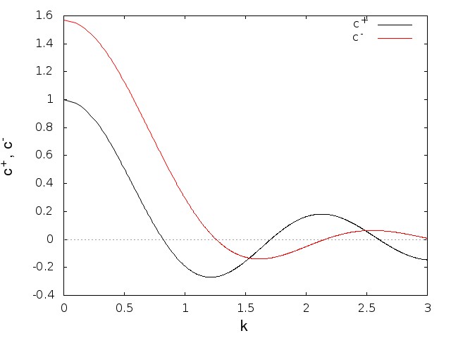
Figure 2: The limit values $c^{\pm}(k),$ with zeros corresponding to the allowed momenta.

As the odd (even) values of $n$ correspond to even (odd) functions with respect to $z\to-z$, a more convenient notation from now on is to label the eigenfunctions by an integer by defining

$$\psi_{2n-1}(z)\equiv\psi_{(k_{2n-1})}^{+}(z)\ ,\qquad\psi_{2n}(z)\equiv\psi_{(k_{2n})}^{-}(z)\ ,\qquad n=1,2,\dots$$ (4.35)

so that the information about the parity of the eigenfunction is encoded in the parity of the integer index.

In the absence of a conformal boundary the eigenfunction $\psi_{(k)}^{\pm}(z)$ has an infinite number of zeros and oscillates as $z\to\infty.$ In this situation a function like $1/\rho^{2}$, that vanishes as $z\to\infty$, can be expanded as an integral over all momenta $k,$ as in (4.17), even if $\psi_{(k)}^{\pm}(z)\centernot\to 0$ as $z\to\infty$ It is the oscillating property of the eigenfunction that produces decoherence and leads to this result.

In contrast, when there is a conformal boundary the eigenfunction $\psi_{(k)}^{\pm}(z)$ has a finite number of zeros and does not oscillate for large $z,$ but rather tends monotonically to a finite limit as $z\to\infty$. For $p=\frac{2}{3}$ the large $z$ behaviour is $\psi_{(k)}^{\pm}(z)\sim c^{\pm}(k)+d^{\pm}(k)/z+\ldots.$ In this situation, the expansion of a function that vanishes at infinity requires all the eigenfunctions in the expansion to also vanish at infinity, so the boundary conditions (4.33) and (4.34) must be imposed.

To make sense of (4.18) we must therefore project to the subspace of allowed eigenfunctions to obtain the form

$$\xi(x_{i},z)=\sum_{n=1}^{\infty}\,\xi_{2n-1}\frac{e^{-k_{2n-1}r}}{r}\psi_{2n-1}(z),$$ (4.36)

where the projection coefficients $\xi_{2n-1}$ are defined by

$$\xi_{2n-1}=\frac{1}{(\psi_{2n-1},\psi_{2n-1})}\int_{0}^{\infty}(\psi^{+}_{(k)},\psi_{2n-1})\,dk,$$ (4.37)

using the inner product

$$(\psi,\widetilde{\psi})=\int_{-\infty}^{\infty}\frac{1}{H^{1/2}}\psi\widetilde{\psi}\,dz.$$ (4.38)

This is the inner product in which the eigenfunctions $\psi_{n}$ are orthogonal, $(\psi_{m},\psi_{n})\propto\delta_{mn}.$

The discretization (4.36) has an important consequence. As $k_{1}>0$, the large distance decay is now exponential not algebraic. Since $\widehat{A}_{0}$ is the field dual to the baryon current of the boundary theory, this means that the baryon form factors, at least within this linear approximation, decay exponentially.

Another consequence of the discretization appears when we retract back to the flat regime, as it converts the identity (4.17) into the approximation

$$\frac{1}{\rho^{2}}\simeq\sum_{n=1}^{\infty}\,\xi_{2n-1}\frac{e^{-k_{2n-1}r}}{r}\cos(k_{2n-1}z),$$ (4.39)

due to the projection to an incomplete subset of eigenfunctions. However, in the almost flat region $|z|\ll 1$ the large momenta modes are the most important in reconstructing the function ${1}/{\rho^{2}},$ so this discretization does not affect the validity of the small instanton approximation.

A similar story applies to the projection of the non-abelian potential. In particular, the relations (4.32) become

$$A^{(1-)}_{i}=\frac{\mu^{2}}{2}{\sigma}_{i}\sum_{n=0}^{\infty}\xi_{2n}\frac{e^{-k_{2n}r}}{r}k_{2n}^{2}\psi_{2n}(z),\qquad A^{(1+)}_{z}=\frac{\mu^{2}}{2}{\sigma}_{i}\sum_{n=0}^{\infty}\xi_{2n}\partial_{i}\frac{e^{-k_{2n}r}}{r}\phi_{2n}{(z)},$$ (4.40)

where $\phi_{n}(z)=\partial_{z}\psi_{n}(z)$ using our new notation. An expression for the projection coefficients $\xi_{2n}$ will be given below, but first we draw attention to an important point. An additional mode has been included in the expansions (4.40), where we have defined $k_{0}=0.$ The associated zero mode is

$$\psi_{0}(z)=\int_{0}^{z}\frac{1}{H(z)^{3/2}}\,dz\quad\mbox{with}\quad\phi_{0}(z)=\frac{1}{H(z)^{3/2}}.$$ (4.41)

Note that $\psi_{0}(\infty)\neq 0,$ hence this mode was excluded from the earlier considerations. However, since $k_{0}=0$ this mode does not contribute to $A_{i}^{(1-)}$ due to the $k_{2n}^{2}$ factor in the first formula in (4.40). Thus the boundary condition on the field strength (that the parallel components vanish at the conformal boundary) remains satisfied. The eigenfunction $\psi_{0}$, with zero eigenvalue, is associated with the massless pion and contributes through the inclusion in $A_{z}^{(1+)}$ of the mode $\phi_{0},$ which vanishes at infinity. For the Sakai-Sugimoto model $p=\frac{2}{3}$ which gives $\phi_{0}=1/(1+z^{2})$ and $\psi_{0}=\tan^{-1}z$ with $\psi_{0}(\infty)=\frac{\pi}{2}.$

From the second formula in (4.40) the projection coefficients are given by a similar expression to (4.37), namely

$$\xi_{2n}=\frac{1}{\langle\phi_{2n},\phi_{2n}\rangle}\int_{0}^{\infty}\langle\phi^{+}_{(k)},\phi_{2n}\rangle\,dk,$$ (4.42)

using the appropriate inner product

$$\langle\phi,\widetilde{\phi}\rangle=\int_{-\infty}^{\infty}{H^{3/2}}\phi\widetilde{\phi}\,dz,$$ (4.43)

for orthogonality $\langle\phi_{m},\phi_{n}\rangle\propto\delta_{mn}.$

For $n\neq 0,$ an integration by parts, together with an application of the defining equation for the eigenfunctions (4.19), proves the identity

$$\langle\phi_{(k)}^{+},\phi_{2n}\rangle=(k^{2}\psi_{(k)}^{-},\psi_{2n}).$$ (4.44)

Using this identity gives the first projection formula in (4.40), which completes the derivation.

In summary, the conclusion from the linear analysis in curved space is that at large three-dimensional distance, $r\gtrsim 1$, all terms decay exponentially, except the algebraic decay associated with the pion field. Explicitly,

$$A^{(1)}_{z}=-\frac{\xi_{0}\mu^{2}}{2}\,\frac{\sigma_{i}\widehat{x}_{i}}{r^{2}}\,\phi_{0}(z)+{\cal O}\bigg{(}\frac{e^{-k_{2}r}}{r}\bigg{)},\quad A^{(1)}_{i}={\cal O}\bigg{(}\frac{e^{-k_{1}r}}{r}\bigg{)},\quad\widehat{A}^{(1)}_{0}={\cal O}\bigg{(}\frac{e^{-k_{1}r}}{r}\bigg{)},$$ (4.45)

where $\widehat{x}_{i}=x_{i}/r.$ In the following subsection we shall show that the linear result (4.45) cannot be used to conclude anything about the asymptotic tail of the soliton fields. In particular, by extending it to arbitrarily large values of the radius $r,$ it leads to incorrect conclusions regarding the exponential decay of physical quantities of the baryon, such as the baryon density and electromagnetic form factors. We shall see that these linear results do have a region of validity, but this region does not include arbitrarily large values of the radius, since nonlinear terms then dominant over the linear result (4.45). This is the source of several erroneous computations and conclusions in the literature.

4.4 Noncommutativity of the large $\Lambda$ and large $r$ limits

As we saw in the previous subsection, if we take the leading order term in the $1/\Lambda$ expansion and then expand again to find the large $r$ behaviour, then the dominant contribution is from the pion field. It produces an ${\cal O}(1/r^{2})$ term that appears only in the $A_{z}$ component of the gauge potential and not in the $A_{i}$ or $\widehat{A}_{0}$ components, which decay exponentially. It is crucial to note the order of the limits here: first we take the large $\Lambda$ limit, which selects the linear term ${\cal A}^{(1)},$ and then we consider the large $r$ limit. This ordering assumes that the linearized fields given in (4.45) provide the dominant contribution at large $r.$ If this assumption is to be valid then it requires that all higher order terms in the $1/\Lambda$ expansion of $A_{i}$ and $\widehat{A}_{0}$ decay exponentially with $r.$ In this subsection we prove that this requirement is not satisfied and hence the linear result is not valid at large $r.$ We begin by assuming the linear result is valid and then find a contradiction.

For the remainder of the computations in this subsection we ignore all terms that decay exponentially with $r,$ as we are interested in the details of the algebraic decay. With the exponential terms neglected, $A_{i}=\widehat{A}_{0}=0.$ From (4.45), the only non-zero components of the field strength at linear order in $1/\Lambda$ are

$$F^{(1)}_{iz}=\frac{\xi_{0}\mu^{2}}{2}\phi_{0}\sigma_{j}\partial_{i}\partial_{j}\bigg{(}\frac{1}{r}\bigg{)}.$$ (4.46)

In particular, this means that at the linear level the instanton charge density decays exponentially.

The field equations (2.13) and (2.14) now become

$$D_{z}\left(H^{3/2}F_{iz}\right)=0,\qquad\qquad D_{i}F_{iz}=0.$$ (4.47)

We can check that they are satisfied at linear order

$$\partial_{z}\left(H^{3/2}F^{(1)}_{iz}\right)=0,\qquad\qquad\partial_{i}F^{(1)}_{iz}=0,$$ (4.48)

using (4.46) and the identities

$$\partial_{z}\left(H^{3/2}\phi_{0}\right)=0,\qquad\qquad\partial_{i}\partial_{i}\left(\frac{1}{r}\right)=0.$$ (4.49)

However, a problem arises at the next order in the $1/\Lambda$ expansion. At second order the first equation in (4.47) becomes

$$\partial_{z}(H^{3/2}\partial_{i}A_{z}^{(2)})+iH^{3/2}[A_{z}^{(1)},F^{(1)}_{iz}]=0,$$ (4.50)

which simplifies to

$$\partial_{z}(H^{3/2}\partial_{i}A_{z}^{(2)})=-\frac{1}{2}\xi_{0}^{2}\mu^{4}\phi_{0}\varepsilon_{ijk}\frac{\widehat{x}_{j}}{r^{5}}\sigma_{k}.$$ (4.51)

This equation determines the $z$ dependence of $A_{z}^{(2)}$ to be

$$A_{z}^{(2)}=-\frac{1}{2}\xi_{0}^{2}\mu^{4}\phi_{0}\psi_{0}\beta,$$ (4.52)

where $\beta$ is independent of $z$ and solves the equation

$$\partial_{i}\beta=\varepsilon_{ijk}\frac{\widehat{x}_{j}}{r^{5}}\sigma_{k}.$$ (4.53)

However, it is easy to prove that there are no solutions to (4.53). Defining the right hand side of (4.53) to be $\Xi_{i},$ the existence of a solution $\beta$ requires the zero curvature condition $\partial_{i}\Xi_{j}-\partial_{j}\Xi_{i}=0,$ which is easily calculated and does not vanish.

This proves that it is impossible to extend the linear result (4.45) to higher order in $1/\Lambda$ if $A_{i}$ and $\widehat{A}_{0}$ decay exponentially with $r.$ Terms in $A_{i}$ and $\widehat{A}_{0}$ with algebraic decay are required beyond linear order for a consistent expansion. As a result, at large radius these higher order terms in $1/\Lambda$ dominate over the exponential terms at linear order. The upshot is that the linear result is not valid at large radius and gives incorrect results for physical quantities, such as the baryon density, the abelian electric field and electromagnetic form factors. In the following subsection we derive the correct extension of the linear expansion (4.45) for large $r.$

4.5 A nonlinear expansion at large $r$

The $1/\Lambda$ expansion will still play a role in this subsection, but to obtain the correct large $r$ behaviour it is vital to include higher order terms beyond the linear contribution ${\cal A}^{(1)}.$ We reverse the order of the limits in the previous subsection by first considering the large $r$ limit and then performing the $1/\Lambda$ expansion. Explicitly, we keep the leading order terms in a $1/r$ expansion at each order in a $1/\Lambda$ expansion. As in the previous subsection, we ignore all exponentially decaying terms, so from (4.45) the expansion starts with the linear term in $1/\Lambda$

$$A^{(1)}_{z}=-\frac{\xi_{0}\mu^{2}}{2}\,\frac{\sigma_{i}\widehat{x}_{i}}{r^{2}}\,\phi_{0},\qquad A^{(1)}_{i}=0,\qquad\widehat{A}^{(1)}_{0}=0.$$ (4.54)

As confirmed previously, the field equations are satisfied at linear order. At second order the field equation (2.13) becomes

$$\partial_{z}(H^{3/2}F^{(2)}_{zi})+iH^{3/2}[A^{(1)}_{z},F^{(1)}_{zi}]+H^{-1/2}\partial_{j}F^{(2)}_{ji}=0.$$ (4.55)

At large $r$ the final term in this expression is of lower order in a $1/r$ expansion than the first and may be neglected. This leaves

$$\partial_{z}(H^{3/2}(\partial_{i}A^{(2)}_{z}-\partial_{z}A^{(2)}_{i}))+iH^{3/2}[A^{(1)}_{z},F^{(1)}_{iz}]=0.$$ (4.56)

As we saw in the previous subsection, it is impossible to solve this equation with $A^{(2)}_{i}=0.$ We now derive the solution for $A^{(2)}_{i}$ in the gauge $A_{z}^{(2)}=0,$ when (4.56) becomes

$$\partial_{z}(H^{3/2}\partial_{z}A_{i}^{(2)})=\frac{1}{2}\xi_{0}^{2}\mu^{4}\phi_{0}\varepsilon_{ijk}\frac{\widehat{x}_{j}}{r^{5}}\sigma_{k}.$$ (4.57)

The $z$ dependence factors as

$$A_{i}^{(2)}=\eta\frac{1}{2}\xi_{0}^{2}\mu^{4}\varepsilon_{ijk}\frac{\widehat{x}_{j}}{r^{5}}\sigma_{k},$$ (4.58)

where $\eta(z)$ solves the equation

$$\partial_{z}(H^{3/2}\partial_{z}\eta)=\phi_{0}.$$ (4.59)

Using $\phi_{0}=1/H^{3/2}=\partial_{z}\psi_{0},$ this equation may be integrated once to give

$$\partial_{z}\eta=\psi_{0}\phi_{0},$$ (4.60)

which is solved by

$$\eta=\frac{1}{2}\psi_{0}^{2}-\frac{\pi^{2}}{8},$$ (4.61)

where the constant of integration has been fixed by the requirement that $\eta(\infty)=0$ and we have used the earlier result that $\psi_{0}(\infty)=\frac{\pi}{2}$ for the Sakai-Sugimoto model with $p=\frac{2}{3}.$

The $ij$ component of the field strength has a contribution at second order

$$F_{ij}^{(2)}=-\frac{\xi_{0}^{2}\mu^{4}\eta}{r^{6}}\big{(}\varepsilon_{ijk}+3\widehat{x}_{l}(\varepsilon_{ikl}\widehat{x}_{j}-\varepsilon_{jkl}\widehat{x}_{i})\big{)}\sigma_{k}$$ (4.62)

and thus the term proportional to the instanton charge density

$${\cal I}=\varepsilon_{IJKL}\,{\rm tr}\,({F}_{IJ}{F}_{KL})$$ (4.63)

is generated at third order in $1/\Lambda$

$${\cal I}^{(3)}=4\varepsilon_{ijk}\,{\rm tr}\left(F^{(2)}_{ij}F^{(1)}_{kz}\right)=-\frac{48\xi_{0}^{3}\mu^{6}\phi_{0}\eta}{r^{9}}\propto\frac{1}{\Lambda^{3}r^{9}}.$$ (4.64)

The abelian field $\widehat{A}_{0}$ is sourced by ${\cal I}$ with a coupling $1/\Lambda$, and thus it is generated at fourth order. The equation for $\widehat{A}_{0}$ in radial coordinates is

$$H^{-1/2}\partial_{r}\left(r^{2}\partial_{r}\widehat{A}_{0}\right)+r^{2}\partial_{z}\left(H^{3/2}\partial_{z}\widehat{A}_{0}\right)=\frac{1}{\Lambda}r^{2}{\cal I},$$ (4.65)

so the fourth order term satisfies

$$H^{-1/2}\partial_{r}\left(r^{2}\partial_{r}\widehat{A}_{0}^{(4)}\right)+r^{2}\partial_{z}\left(H^{3/2}\partial_{z}\widehat{A}_{0}^{(4)}\right)=-\frac{48\xi_{0}^{3}\mu^{6}\phi_{0}\eta}{\Lambda r^{7}}.$$ (4.66)

Applying the ansatz

$$\widehat{A}_{0}^{(4)}=-\frac{48\xi_{0}^{3}\mu^{6}}{\Lambda r^{9}}\chi,$$ (4.67)

with $\chi(z)$, and neglecting subleading terms in $1/r$, we obtain the equation

$$\partial_{z}\left(H^{3/2}\partial_{z}\chi\right)=\phi_{0}\eta,$$ (4.68)

which must be solved subject to the boundary conditions $\chi(\pm\infty)=0$. The solution is easily obtained by using $\psi_{0}$ as the independent coordinate rather than $z$, as equation (4.68) then simplifies to

$$\frac{\partial^{2}\chi}{\partial\psi_{0}^{2}}=\frac{1}{2}\psi_{0}^{2}-\frac{\pi^{2}}{8}.$$ (4.69)

The unique solution satisfying the above boundary conditions is

$$\chi=\frac{1}{24}\bigg{(}\psi_{0}^{4}-6\bigg{(}\frac{\pi}{2}\bigg{)}^{2}\psi_{0}^{2}+5\bigg{(}\frac{\pi}{2}\bigg{)}^{4}\bigg{)},$$ (4.70)

to give

$$\widehat{A}_{0}^{(4)}=-\frac{2\xi_{0}^{3}\mu^{6}}{\Lambda r^{9}}\bigg{(}\psi_{0}^{4}-6\bigg{(}\frac{\pi}{2}\bigg{)}^{2}\psi_{0}^{2}+5\bigg{(}\frac{\pi}{2}\bigg{)}^{4}\bigg{)}.$$ (4.71)

We have now achieved our aim of determining the leading order large $r$ behaviour of all the fields and their relation to the small instanton approximation. Namely,

$$A_{z}=-\frac{1}{2}\xi_{0}\mu^{2}\frac{\widehat{x}_{i}\sigma_{i}}{r^{2}}\phi_{0}+\ldots,\qquad A_{i}=\frac{1}{2}\xi_{0}^{2}\mu^{4}\varepsilon_{ijk}\frac{\widehat{x}_{j}\sigma_{k}}{r^{5}}\eta+\ldots,\qquad\widehat{A}_{0}=-\frac{48\xi_{0}^{3}\mu^{6}}{\Lambda r^{9}}\chi+\ldots$$ (4.72)

Note the significant difference in the rate of decay of the abelian field $\widehat{A}_{0}$ in the $r$ and $z$ directions, since $\chi$ decays only as ${\cal O}(\frac{1}{z})$ for large $z.$

4.6 The emergence of a new scale

We now describe the way in which the results we have obtained imply the existence of a new large scale, in which the behaviour of the $A_{i}$ and $\widehat{A}_{0}$ components are dominated by nonlinear terms. Recall that the $1/\Lambda$ expansion at large $r$ takes the form

$$A_{z} = A^{(1)}_{z}+\dots$$

$$A_{i} = \phantom{A^{(2)}_{z}+}A^{(2)}_{i}+\dots$$

$$\widehat{A}_{0} = \phantom{A^{(1)}_{z}+A^{(3)}_{i}+\ \ \ \ \ }\widehat{A}_{0}^{(4)}+\dots$$ (4.73)

where $A_{i}$ starts only at second order and $\widehat{A}_{0}$ starts only at fourth order, once exponentially decaying terms are neglected. However, we need to determine the scale at which it is appropriate to neglect these exponentially decaying terms, so that the nonlinear terms with algebraic decay dominate over the linear result.

The new scale is where the linear terms in the $1/\Lambda$ expansion of $A_{i}$ and $\widehat{A}_{0}$ are comparable to the higher order terms, that is, $A^{(1)}_{i}\sim A^{(2)}_{i},\ \ \widehat{A}^{(1)}_{0}\sim\widehat{A}^{(4)}_{0}.$ From our earlier results this is equivalent to

$$\frac{e^{-k_{1}r}}{\Lambda r}\sim\frac{1}{\Lambda^{2}r^{5}},\ \frac{1}{\Lambda^{4}r^{9}},$$ (4.74)

so a new length scale appears at ${r}\sim\log{\Lambda},$ or more generally ${r}\sim L\log{\Lambda},$ if we reinstate the scale $L.$ Note that this is a large scale for large $\Lambda.$ It is the scale beyond which the asymptotic fields, of the form (4.73), are applicable to describe the tail of the soliton.

It is common to define the size of a soliton’s core by reference to the region beyond which the fields of the asymptotic tail provide a good approximation to the fields of the soliton. If such a definition is used then the soliton is large at large ’t Hooft coupling. This is in stark contrast to the commonly stated result that the soliton has a small size, which results by defining the size via comparison with the approximate self-dual instanton. The size of the Sakai-Sugimoto soliton is therefore a more complicated issue than previously realized.

In summary, there are three important scales in the problem. The scale of the self-dual instanton, $L/\sqrt{\Lambda}$, the radius of curvature $L$, and the new scale of order $L\log{\Lambda}$. The various approximations discussed in this paper are valid in different regions, some of which are contiguous and therefore allow the different approximations to be related. These different regions correspond to the treatment of space as flat or curved and the treatment of the partial differential equations as linear or nonlinear. Schematically, we may summarise the situation as:

$$0< \rho \lesssim L/\sqrt{\Lambda},\ \qquad\qquad\mbox{\rm flat and nonlinear}$$

$$L/\sqrt{\Lambda}\lesssim \rho \lesssim L,\ \qquad\qquad\qquad\mbox{\rm flat and linear}$$

$$L\lesssim \rho \lesssim L\log{\Lambda},\qquad\qquad\mbox{\rm curved and linear}$$

$$L\log{\Lambda}\lesssim \rho$$ curved and nonlinear. (4.75)

The appearance of the final region is a slightly unusual feature due to the fact that at large radius nonlinear terms dominate over linear terms, despite the fact that these terms are small. This has led to some confusion by previous authors, who have incorrectly assumed the more generic behaviour that when functions become small the system enters a linear regime.

4.7 The Cherman-Ishii expansion

Cherman and Ishii [13] have performed a large $r$ expansion to obtain the asymptotic fields of the Sakai-Sugimoto soliton, based on a method first applied in a different holographic model [11]. They found that the fields have an algebraic decay with a form that satisfies the model independent form factor relations described in [12]. However, they were only able to implement their approach by introducing a UV cutoff and the limit as this cutoff is removed is problematic: prompting them to speculate on possible resolutions that include holographic renormalization and boundary counterterms. In this subsection we describe the relation between our asymptotic fields and those of the Cherman-Ishii expansion. Although the Cherman-Ishii fields appear to have a more complicated form than our expressions, we shall show that they are gauge equivalent. Moreover, we shall see that their required UV cutoff is merely a gauge artifact that is a consequence of a gauge choice that is incompatible with the holographic boundary conditions. Although our asymptotic expansion turns out to be equivalent to the Cherman-Ishii expansion, our derivation has the advantage that the constant appearing in the expansion is directly related to the self-dual instanton, whereas it appears simply as an unknown constant in the Cherman-Ishii expansion, even after a gauge transformation to remove the spurious UV cutoff.

First we highlight the relevant issue concerning the choice of gauge. The required condition at the conformal boundary, that the field strength has vanishing parallel components, is gauge invariant. In the AdS/CFT dictionary the gauge potential $A_{i}$ at the boundary corresponds to the source for the related current. If $F_{ij}$ is zero at the boundary, then it is always possible to choose a gauge in which $A_{i}$ is also set to zero at the boundary (so that the sources vanish). The chosen gauge for our expansion is already in this form. The starting point of our linear expansion (4.54) has $A_{i}^{(1)}=0$, moreover none of the higher order terms give a contribution at the boundary, so $A_{i}$ vanishes there. This is why we have no need for a UV cutoff.

The expansion strategy followed in [13] has led to some confusion about the choice of gauge because they directly perform a radial expansion in $1/r$ and do not consider an expansion in $1/\Lambda$. They start their expansion with a dominant term at large $r$ given by

$$A_{z}=\beta\frac{\sigma_{j}\widehat{x}_{j}}{r^{2}}+\ldots$$ (4.76)

where $\beta$ is a constant that is left arbitrary and cannot be determined using their approach. The crucial point here is that this term is independent of $z$. All the other terms in the $1/r$ expansion are then derived on top of this one, choosing step by step a gauge in which $A_{i}=0$ at the boundary. However, by postulating the leading term (4.76) this implicitly contains a gauge choice, which is not necessarily compatible with the choice of gauge in which $A_{i}=0$ at the boundary. In fact it turns out that, generically, the only way to have $A_{i}$ vanishing at the boundary is to introduce a fictitious UV cutoff. The need for a cutoff simply reflects the fact that the gauge implicitly chosen by the starting point (4.76) is not a good one.

To relate our expansion to that of Cherman and Ishii we shall take our leading order result, given by the pion tail (4.54), and attempt to convert it to a gauge in which (4.76) holds. The first step is to perform the gauge transformation given by

$$G_{1}=\exp{\left(-\frac{i}{2}\xi_{0}\mu^{2}\frac{\sigma_{j}\widehat{x}_{j}}{r^{2}}\psi_{0}(z)\right)},$$ (4.77)

which results in

$$A_{z}^{(1)}=0,\qquad\qquad A_{i}^{(1)}=\frac{\xi_{0}\mu^{2}}{2r^{3}}(\sigma_{i}-3\sigma_{j}\widehat{x}_{i}\widehat{x}_{j})\psi_{0}(z),$$ (4.78)

so that the pion tail is transferred entirely into the $A_{i}$ component.

This is a perfectly legitimate gauge, but it does not have vanishing sources at the boundary, because $\psi_{0}(\infty)\neq 0.$ A way to resolve this issue is to introduce a UV cutoff, $z_{UV},$ and perform second gauge transformation given by

$$G_{2}=\exp{\left(\frac{i}{2}\xi_{0}\mu^{2}\frac{\sigma_{j}\widehat{x}_{j}}{r^{2}}\frac{z\psi_{0}(z_{UV})}{z_{UV}}\right)},$$ (4.79)

so that (4.78) becomes

$$A_{z}^{(1)}=-\frac{\xi_{0}\mu^{2}}{2}\,\frac{\sigma_{j}\widehat{x}_{j}}{r^{2}}\frac{\psi_{0}(z_{UV})}{z_{UV}},\qquad A_{i}^{(1)}=\frac{\xi_{0}\mu^{2}}{2r^{3}}(\sigma_{i}-3\sigma_{j}\widehat{x}_{i}\widehat{x}_{j})\bigg{(}\psi_{0}(z)-\frac{z\psi_{0}(z_{UV})}{z_{UV}}\bigg{)}.$$ (4.80)

Now $A_{i}^{(1)}$ vanishes at the UV boundary $z=z_{UV}$ and $A_{z}^{(1)}$ has the form (4.76) with $\beta=-\xi_{0}\mu^{2}\psi_{0}(z_{UV})/(2z_{UV}).$ This demonstrates the equivalence between the Cherman-Ishii expansion and our simpler version (4.54) and explains how the UV cutoff terms are simply gauge artefacts.

The conclusion is that the correct gauge to have vanishing sources is in fact (4.54) with no term like (4.76). In the Cherman-Ishii expansion there are other terms, of higher order in $1/r$ and linear in $1/\Lambda$, that can also be removed by a gauge transformation, leaving the physical terms that correspond to our second order and fourth order terms (4.58) and (4.71). In particular, formula (4.71) for the leading order large $r$ behaviour of $\widehat{A}_{0},$ does not depend on the choice of gauge for the non-abelian fields and coincides with the one given in [14], which is a correction of the expression in [13] (as this contains an error).

In the recent preprint [14], which appeared on the arXiv during the preparation of this manuscript, it is argued that the UV cutoff is a kind of coordinate singularity that can be removed by a very specific change of variable for the holographic coordinate. However, the interpretation as a coordinate singularity is not the underlying explanation but is a pure coincidence, as follows. In the right gauge, the correct starting point for the expansion of $A_{z}$ is $A_{z}^{(1)}$ given by (4.54), which has a $z$ dependence proportional to $\phi_{0}(z).$ The specific change of coordinate identified in [14] is to use $\widetilde{z}=\psi_{0}(z)$ as the holographic variable. The correct dependence of $A_{z}^{(1)}$ maps to an $A_{\widetilde{z}}^{(1)}$ that is independent of $\widetilde{z},$ and hence is of the form (4.76), simply because this specific choice of $\widetilde{z}$ obeys $d\widetilde{z}/dz=\phi_{0},$ which cancels the $z$-dependent factor of $\phi_{0}$ in $A_{z}.$ Independence of the holographic coordinate happens only for this specific choice of coordinate and for a generic coordinate the correct formula is obtained from (4.54).

5 Numerical computations

In this section we describe our numerical scheme for the computation of the Sakai-Sugimoto soliton, together with some of the results it generates. We shall see that the numerical results are in good agreement with the analytical approximations discussed in the previous sections.

Static $SO(3)$ symmetric fields have the form [15, 16]

$$A_{j}=\bigg{(}\frac{1+\Phi_{2}}{r}\varepsilon_{jak}\widehat{x}_{k}+\frac{\Phi_{1}}{r}(\delta_{ja}-\widehat{x}_{j}\widehat{x}_{a})+a_{r}{\widehat{x}_{j}\widehat{x}_{a}}\bigg{)}\frac{\sigma_{a}}{2},\quad A_{z}=a_{z}\widehat{x}_{a}\frac{\sigma_{a}}{2},\quad\widehat{A}_{0},$$ (5.1)

where the fields $\Phi_{1},\Phi_{2},a_{r},a_{z},\widehat{A}_{0}$ are functions of $r$ and $z.$

Writing $\Phi=\Phi_{1}+i\Phi_{2},$  $f_{rz}=\partial_{r}a_{z}-\partial_{z}a_{r}$ and $D_{r}\Phi=\partial_{r}\Phi-ia_{r}\Phi,$ the expression for the baryon number becomes

$$B=-\int_{0}^{\infty}dr\int_{-\infty}^{\infty}dz\ \frac{1}{2\pi}\bigg{\{}f_{rz}(1-|\Phi|^{2})+i(D_{r}\Phi\overline{D_{z}\Phi}-\overline{D_{r}\Phi}D_{z}\Phi)\bigg{\}}.$$ (5.2)

In terms of these variables, the energy obtained from the action (2.12) has three terms, $E=4\pi(E_{SU(2)}+E_{U(1)}+E_{CS}),$ where

$$E_{SU(2)}=\int_{0}^{\infty}dr\int_{-\infty}^{\infty}dz\ \bigg{\{}H^{-\frac{1}{2}}|D_{r}\Phi|^{2}+H^{\frac{3}{2}}|D_{z}\Phi|^{2}+\frac{r^{2}H^{\frac{3}{2}}}{2}f_{rz}^{2}+\frac{H^{-\frac{1}{2}}}{2r^{2}}(1-|\Phi|^{2})^{2}\bigg{\}},$$ (5.3)

$$E_{U(1)}=-\int_{0}^{\infty}dr\int_{-\infty}^{\infty}dz\ \bigg{\{}\frac{1}{2}r^{2}\bigg{(}H^{-\frac{1}{2}}(\partial_{r}\widehat{A}_{0})^{2}+H^{\frac{3}{2}}(\partial_{z}\widehat{A}_{0})^{2}\bigg{)}\bigg{\}},$$ (5.4)

$$E_{CS}=-\frac{1}{\Lambda}\int_{0}^{\infty}dr\int_{-\infty}^{\infty}dz\ \bigg{\{}4\widehat{A}_{0}\bigg{(}f_{rz}(1-|\Phi|^{2})+i(D_{r}\Phi\overline{D_{z}\Phi}-\overline{D_{r}\Phi}D_{z}\Phi)\bigg{)}\bigg{\}}.$$ (5.5)

For reference, the flat space self-dual instanton is given by

$$\Phi=\frac{2rz+i(r^{2}-z^{2}-\mu^{2})}{\rho^{2}+\mu^{2}},\quad a_{r}=\frac{2z}{\rho^{2}+\mu^{2}},\quad a_{z}=\frac{-2r}{\rho^{2}+\mu^{2}},$$ (5.6)

where, as earlier, $\rho^{2}=r^{2}+z^{2}.$ The required soliton has $B=1$ and is a vortex in the reduced theory on the half-plane $r\geq 0.$ On the boundary $\{r=0\}\cup\{\rho=\infty\}$ the complex field $\Phi$ has unit modulus and its phase varies by $2\pi$ around the boundary. Setting $\mu=0$ in (5.6) gives the fields

$$\Phi=\frac{2rz+i(r^{2}-z^{2})}{\rho^{2}},\qquad a_{r}=\frac{2z}{\rho^{2}},\qquad a_{z}=\frac{-2r}{\rho^{2}},\qquad$$ (5.7)

which are pure gauge but have a singularity at the point $\rho=0.$ These fields satisfy $|\Phi|=1$ and $D_{r}\Phi=D_{z}\Phi=f_{rz}=0,$ which are the natural boundary conditions to impose as $\rho\rightarrow\infty.$ In particular, the phase of $\Phi$ varies by $2\pi$ along this boundary. The boundary conditions along the line $r=0$ are $\Phi=-i,\ D_{r}\Phi=D_{z}\Phi=0,$ which are those of the finite size self-dual instanton. A series expansion of the field equations around $r=0$ confirms that these are the correct boundary conditions as $r\rightarrow 0,$ together with $\partial_{r}\widehat{A}_{0}=0.$ In summary, the boundary conditions at $r=0$ are given by

$$\Phi=-i,\quad a_{r}=\partial_{r}\Phi_{1},\quad a_{z}=0,\quad\partial_{r}\widehat{A}_{0}=0,$$ (5.8)

and as $\rho\rightarrow\infty$ the fields are given by (5.7) together with $\widehat{A}_{0}\rightarrow 0.$

The field equations that follow from the variation of the energy $E$ are solved using a heat flow method. For the fields $\Phi_{1},\Phi_{2},a_{r},a_{z}$ this corresponds to gradient flow associated with the energy $E_{SU(2)}+E_{CS},$ in the Coulomb gauge $\partial_{r}a_{r}+\partial_{z}a_{z}=0.$ For $\widehat{A}_{0}$ the heat flow corresponds to gradient flow associated with the energy $-E_{U(1)}-E_{CS},$ where the negative signs are due to the negative sign that appears in front of the energy (5.4), arising because $\widehat{A}_{0}$ is the time component of a gauge potential. The problem may be viewed as a constrained energy minimization, where the energy $E_{SU(2)}+E_{CS}$ is to be minimized subject to the constraint that $\widehat{A}_{0}$ satisfies the field equation

$$\frac{1}{r^{2}H^{1/2}}\partial_{r}(r^{2}\partial_{r}\widehat{A}_{0})+\partial_{z}(H^{3/2}\partial_{z}\widehat{A}_{0})=\frac{4}{\Lambda r^{2}}\bigg{\{}f_{rz}(1-|\Phi|^{2})+i(D_{r}\Phi\overline{D_{z}\Phi}-\overline{D_{r}\Phi}D_{z}\Phi)\bigg{\}},$$ (5.9)

which is a curved space Poisson equation sourced by the instanton charge density.

As an initial condition for the numerical relaxation the self-dual instanton fields (5.6) are taken with a spatially dependent size $\mu(r,z)$ so that $\mu(0,0)\neq 0$ but $\mu(r,z)=0$ for sufficiently large $\rho.$ For $\widehat{A}_{0}$ the initial condition is that it vanishes everywhere.

As we have seen from the analysis in the previous sections, and will be confirmed by the numerical computations in this section, the fields decay more slowly in the $z$ direction than in the $r$ direction, due to the warped metric. As a result, it turns out to be computationally efficient to perform the change of variable $z=\tan w,$ so that the infinite domain of $z$ transforms to the finite interval $w\in[-\frac{\pi}{2},\frac{\pi}{2}].$ At the boundaries $w=\pm\frac{\pi}{2}$ the fields (5.7) now give the boundary conditions $\ \Phi=-i,\ a_{r}=a_{z}=\widehat{A}_{0}=0.$

The numerical solution is computed on a grid with a boundary at a finite value $r=r_{\star}.$ The boundary conditions applied at this simulation boundary are that the fields are given by the pure gauge fields (5.7) together with $\widehat{A}_{0}=0,$ that is,

$$\Phi=\frac{2r_{\star}\tan w+i(r_{\star}^{2}-\tan^{2}w)}{r_{\star}^{2}+\tan^{2}w},\quad a_{r}=\frac{2\tan w}{r_{\star}^{2}+\tan^{2}w},\quad a_{z}=-\frac{2r_{\star}}{r_{\star}^{2}+\tan^{2}w},\ \widehat{A}_{0}=0.$$ (5.10)

Note that the $2\pi$ phase winding of $\Phi$ now takes place along the single boundary $r=r_{\star}.$ It has been verified that the solutions are insensitive to the choice of this finite boundary, providing $r_{\star}$ is taken to be sufficiently large. The simulation details depend upon the value of $\Lambda,$ as this sets the scale of the soliton, but for $\Lambda$ of order one a typical grid contains $400\times 200$ points in the $(r,w)$-plane with $r_{\star}=40.$

To display the results of the numerical computations it is convenient to plot the abelian potential $\widehat{A}_{0},$ as this is a scalar quantity that is invariant under $SU(2)$ gauge transformations, and in addition the $U(1)$ gauge freedom is fixed by our earlier prescription that $\widehat{A}_{I}=0$ and $\widehat{A}_{0}\to 0$ as $\rho\to\infty.$ Furthermore, we have the simple explicit expression (3.21) for $\widehat{A}_{0}$ within the flat space self-dual approximation, that can be used to compare to the numerical result.

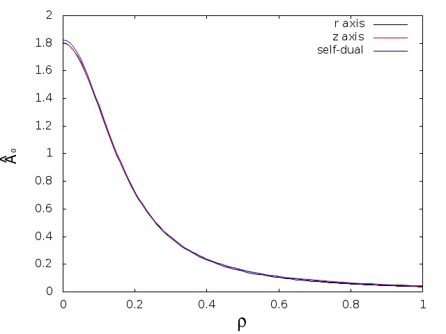
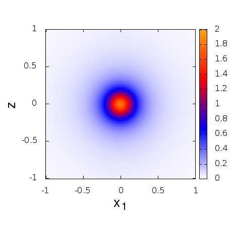
Figure 3: The abelian potential $\widehat{A}_{0}$ for the soliton with $\Lambda=200.$ The left image displays plots of $\widehat{A}_{0}$ along the $r$-axis (black curve) and the $z$-axis (red curve). The flat space self-dual approximation (blue curve) is included for comparison. All three curves are almost indistinguishable as the self-dual field provides a good approximation in this range, apart from a very slight overshoot at the origin. The right image is a plot of $\widehat{A}_{0}$ in the plane $x_{2}=x_{3}=0$ and demonstrates the approximate $SO(4)$ symmetry in this region.

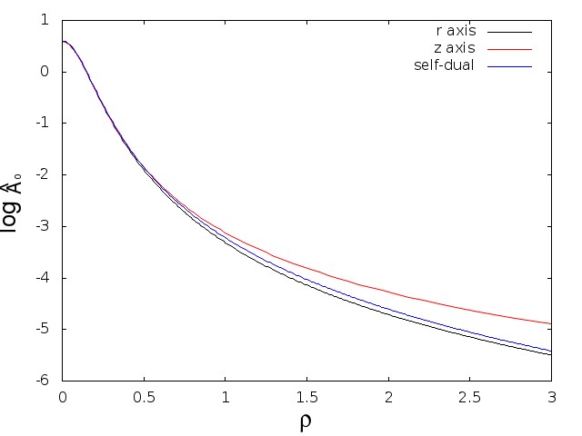
Figure 4: For the soliton with $\Lambda=200,$ the plot displays $\log\widehat{A}_{0}$ against $\rho$ along the $r$-axis (black curve) and the $z$-axis (red curve). The flat space self-dual approximation (blue curve) is included for comparison. There is a faster decay along the $r$-axis than along the $z$-axis.

We first compute the soliton for a large value of $\Lambda,$ where we expect the self-dual instanton to be a good approximation, at least in the region $\rho\lesssim 1.$ Figure 3 displays a plot of $\widehat{A}_{0}$ for the value $\Lambda=200.$ The plot in the left image presents $\widehat{A}_{0}$ along the $r$ and $z$ axes, together with the $SO(4)$ symmetric self-dual instanton approximation (3.21) with the instanton size given by (3.20). All three curves are almost indistinguishable, which confirms that the the self-dual instanton provides a good approximation in this range, for this large value of $\Lambda.$ The plot in the right image presents $\widehat{A}_{0}$ in the plane $x_{2}=x_{3}=0,$ and demonstrates the approximate $SO(4)$ symmetry for $\rho\lesssim 1.$ To see a deviation from the self-dual approximation requires an examination of the region $\rho>1.$ As $\widehat{A}_{0}$ is small in this region then the appropriate quantity to plot is $\log\widehat{A}_{0},$ which is presented in Figure 4 for $0\leq\rho\leq 3.$ The lack of $SO(4)$ symmetry is now more apparent, with a slower decay along the $z$-axis than along the $r$-axis, as predicted by the analytic calculations.

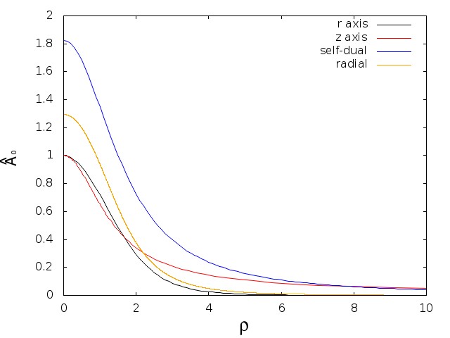
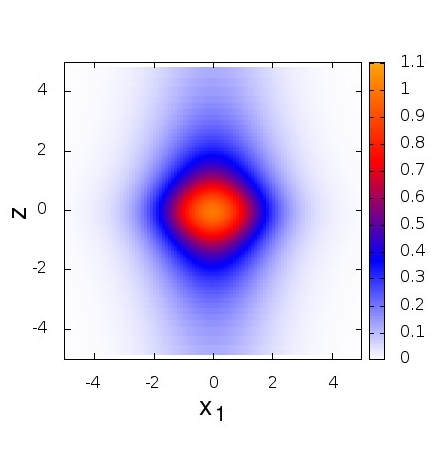
Figure 5: The abelian potential $\widehat{A}_{0}$ for the soliton with $\Lambda=2.$ The left image displays plots of $\widehat{A}_{0}$ along the $r$-axis (black curve) and the $z$-axis (red curve). The flat space self-dual approximation (blue curve) is included for comparison, together with the radial approximation (orange curve). Note the faster decay along the $r$-axis than along the $z$-axis. The right image is a plot of $\widehat{A}_{0}$ in the plane $x_{2}=x_{3}=0.$

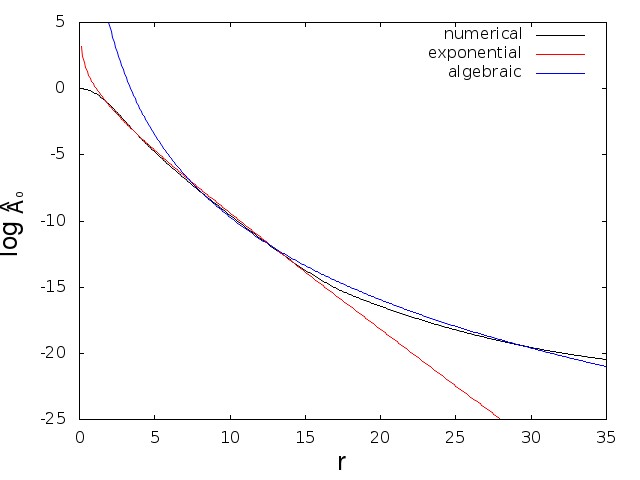
Figure 6: For the soliton with $\Lambda=2,$ the plot displays $\log\widehat{A}_{0}$ against $r$ along the $r$-axis (black curve). The red curve is the exponential decay predicted by the linear approximation in curved space and the blue curve is the algebraic decay predicted by the nonlinear approximation in curved space. Exponential decay is a good approximation in the region $1\lesssim r\lesssim 15$ and algebraic decay is a good approximation in the region $r\gtrsim 8$

To see a demonstrable difference between the self-dual instanton and the numerical solution requires a value of $\Lambda$ that is of order one. This is also the case if we are to provide numerical evidence to support our analytic calculations concerning the applicability of the linear and nonlinear descriptions of the soliton tail in different regions. The most relevant regime from the physical point of view is large $\Lambda,$ but as we have seen, the three length scales involved are of order $1/\sqrt{\Lambda},1,\log\Lambda.$ For large $\Lambda$ this gives a separation of scales that is difficult to encompass within a single simulation. By going to parameter values of $\Lambda$ that are of order one, we can bring these three length scales closer together, so that all three are simultaneously accessible within a feasible simulation.

Figure 5 displays a plot of $\widehat{A}_{0}$ for the value $\Lambda=2.$ The plot in the left image presents $\widehat{A}_{0}$ along the $r$ and $z$ axes, together with the self-dual instanton approximation and the radial approximation described in section 3. The slower decay along the $z$ axis than along the $r$ axis is now clearly visible. The self-dual instanton is a poor approximation for this value of $\Lambda,$ even for small $\rho.$ The radial approximation improves on the self-dual approximation, but there is still a considerable error, as expected from an approximation that assumes $SO(4)$ symmetry. The plot in the right image presents $\widehat{A}_{0}$ in the plane $x_{2}=x_{3}=0,$ and clearly displays the lack of $SO(4)$ symmetry. The abelian potential is stretched out along the $z$ direction, corresponding to the slower rate of decay along the holographic direction, in agreement with the earlier analysis.

To examine the soliton tail, we plot $\log\widehat{A}_{0}$ against $r$ (along the $r$-axis) in Figure 6. Also included in this plot is the leading order exponential decay predicted by the linear analysis, namely $\widehat{A}_{0}={\alpha_{1}e^{-k_{1}r}}/{r},$ and the leading order algebraic decay predicted by the nonlinear analysis, $\widehat{A}_{0}={\alpha_{2}}/{r^{9}},$ where $\alpha_{1,2}$ are constants. It can be seen that exponential decay is a good approximation in the region $1\lesssim r\lesssim 15,$ where the linear regime is valid, and algebraic decay is a good approximation in the region $r\gtrsim 8,$ which is the nonlinear regime. The slight discrepancy between the algebraic form and the numerical result at large $r$ is due to the finite boundary at $r=r_{\star}=40,$ which is not far beyond the range plotted in this figure.

In summary, the numerical results presented in this section demonstrate that the flat space self-dual instanton is a good approximation to the Sakai-Sugimoto soliton for $\rho\lesssim L,$ providing $\Lambda$ is large. Furthermore, we have provided numerical evidence to support the analytic results obtained in this paper regarding the validity of the linear approximation immediately outside the soliton core, together with its breakdown at large scales, where nonlinear terms are dominant.

6 Conclusion

Using a combination of analytic and numerical methods we have investigated the properties of the Sakai-Sugimoto soliton, together with a range of approximations that have been applied to study this soliton. We have determined the regimes of validity of these approximations and shown how they may be related in regions where they overlap. This analysis has clarified the source of some contradictory results in the literature and resolved some outstanding issues, including the applicability of the flat space self-dual instanton, the detailed properties of the asymptotic soliton tail, and the role of the UV cutoff required in previous investigations. We have shown how to relate the asymptotic fields to the self-dual instanton description valid at the core, and revealed the existence of a new large scale, that grows logarithmically with the ’t Hooft coupling, at which the soliton fields enter a nonlinear regime.

The leading order term in the soliton tail is provided by the massless pion field and the classical inter-soliton force has the same structure as in the Skyrme model. Hence there should be an attractive channel that leads to classical multi-soliton bound states that can be quantized within a collective coordinate approximation to provide holographic nuclei. However, these multi-solitons are not expected to have the $SO(3)$ symmetry of the single soliton, so it will be a significant computational challenge to construct these solutions numerically.

References

- [1] M. F. Atiyah and N. S. Manton, “Skyrmions From Instantons,” Phys. Lett. B 222 (1989) 438.
- [2] P. Sutcliffe, JHEP 1008 (2010) 019 [arXiv:1003.0023 [hep-th]].
- [3] T. Sakai and S. Sugimoto, “Low energy hadron physics in holographic QCD,” Prog. Theor. Phys. 113 (2005) 843 [hep-th/0412141].
- [4] T. Sakai and S. Sugimoto, “More on a holographic dual of QCD,” Prog. Theor. Phys. 114 (2005) 1083 [hep-th/0507073].
- [5] D. K. Hong, M. Rho, H. -U. Yee and P. Yi, “Chiral Dynamics of Baryons from String Theory,” Phys. Rev. D 76 (2007) 061901 [hep-th/0701276 [HEP-TH]].
- [6] H. Hata, T. Sakai, S. Sugimoto and S. Yamato, “Baryons from instantons in holographic QCD,” Prog. Theor. Phys. 117 (2007) 1157 [hep-th/0701280 [HEP-TH]].
- [7] K. Hashimoto, T. Sakai and S. Sugimoto, “Holographic Baryons: Static Properties and Form Factors from Gauge/String Duality,” Prog. Theor. Phys. 120 (2008) 1093 [arXiv:0806.3122 [hep-th]].
- [8] D. K. Hong, M. Rho, H. -U. Yee and P. Yi, “Nucleon form-factors and hidden symmetry in holographic QCD,” Phys. Rev. D 77 (2008) 014030 [arXiv:0710.4615 [hep-ph]].
- [9] K. -Y. Kim and I. Zahed, JHEP 0809 (2008) 007 [arXiv:0807.0033 [hep-th]].
- [10] A. Pomarol and A. Wulzer, “Baryon Physics in Holographic QCD,” Nucl. Phys. B 809 (2009) 347 [arXiv:0807.0316 [hep-ph]].
- [11] G. Panico and A. Wulzer, “Nucleon Form Factors from 5D Skyrmions,” Nucl. Phys. A 825 (2009) 91 [arXiv:0811.2211 [hep-ph]].
- [12] A. Cherman, T. D. Cohen and M. Nielsen, “Model Independent Tests of Skyrmions and Their Holographic Cousins,” Phys. Rev. Lett. 103 (2009) 022001 [arXiv:0903.2662 [hep-ph]].
- [13] A. Cherman and T. Ishii, “Long-distance properties of baryons in the Sakai-Sugimoto model,” Phys. Rev. D 86 (2012) 045011 [arXiv:1109.4665 [hep-th]].
- [14] P. Colangelo, J. J. Sanz-Cillero and F. Zuo, “Large-distance properties of holographic baryons,” arXiv:1306.6460 [hep-ph].
- [15] E. Witten, “Some Exact Multi - Instanton Solutions of Classical Yang-Mills Theory,” Phys. Rev. Lett. 38 (1977) 121.
- [16] P. Forgacs and N. S. Manton, “Space-Time Symmetries in Gauge Theories,” Commun. Math. Phys. 72 (1980) 15.