Decoherence and lead induced inter-dot coupling in nonequilibrium electron transport through interacting quantum dots: A hierarchical quantum master equation approach

Abstract

The interplay between interference effects and electron-electron interactions in electron transport through an interacting double quantum dot system is investigated using a hierarchical quantum master equation approach which becomes exact if carried to infinite order and converges well if the temperature is not too low. Decoherence due to electron-electron interactions is found to give rise to pronounced negative differential resistance, enhanced broadening of structures in current-voltage characteristics and an inversion of the electronic population. Dependence on gate voltage is shown to be a useful method of distinguishing decoherence-induced phenomena from effects induced by other mechanisms such as the presence of a blocking state. Comparison of results obtained by the hierarchical quantum master equation approach to those obtained from the Born-Markov approximation to the Nakajima-Zwanzig equation and from the non-crossing approximation to the nonequilibrium Green’s function reveals the importance of an inter-dot coupling that originates from the energy dependence of the conduction bands in the leads and the need for a systematic perturbative expansion.

I Introduction

Electron transport through nanoelectronic devices involves fundamentally important principles which often result in interesting technological applications Kastner (2000); Cuevas and Scheer (2010). Resonant tunneling diodes exhibit a nonlinear current-voltage response, in particular negative differential resistance, due to the quantization of the respective energy levels Chang et al. (1974); Davies et al. (1993); Mizuta and Tanoue (1995). Quantum interference phenomena may be used to control the current flow in three-terminal nanoscale transistors Stafford et al. (2007); Saha et al. (2010) and single-molecule junctions Ballmann et al. (2012). Interaction-driven phenomena such as, for example, static or dynamical Coulomb blockade Kastner (2000); Kießlich et al. (2007); Brun et al. (2012) or the Kondo effect Cronenwett et al. (1998); Goldhaber-Gordon et al. (1998); Liang et al. (2002) also occur. While these phenomena have been studied separately, the interplay between interference phenomena, level quantization and electron-electron interactions in nanoelectronic devices has been less studied and is an important open problem.

Interference effects may arise from a spatial separation of tunneling pathways. As one of many examples one may mention quantum dot arrays set up as Aharonov-Bohm interferometers Holleitner et al. (2001); Aikawa et al. (2004); Holleitner et al. (2002); Ihn et al. (2007). Quasidegenerate energy levels of a single quantum dot may also be understood as separate tunneling pathways and the respective conduction properties interpreted in terms of quantum interference Kalyanaraman and Evans (2002); Ernzerhof et al. (2005); Solomon et al. (2008); Brisker-Klaiman and Peskin (2010); Markussen et al. (2010); Sparks et al. (2011); Brisker-Klaiman and Peskin (2012); Härtle and Thoss (2011a); Ballmann et al. (2012); Härtle et al. (2013a). Both scenarios may be described by Hamiltonians that are nearly identical.

Interference may be strongly affected by electron-electron interactions or coupling between electrons and vibrational modes. Decoherence phenomena arising from electron-vibrational mode coupling in quantum dot systems Marquardt and Bruder (2003); Ueda et al. (2010) or single-molecule junctions Härtle et al. (2011, 2013a) have been studied; one striking result is a pronounced temperature dependence of the current Ballmann et al. (2012); Härtle et al. (2013a, b). In quantum dot arrays, interference effects are suppressed by spin-flip processes König and Gefen (2001); Aikawa et al. (2004); König and Gefen (2002). A similar effect is observed in InSb nanowires, where interaction- or correlation-induced resonances occur Meden and Marquardt (2006); Lee and Kim (2007); Kashcheyevs et al. (2009); Nilsson et al. (2010).

In this article, we investigate the interrelation between interference effects and electron-electron interactions in a nonequilibrium nanoelectronic device modeled as a spinless two-orbital Anderson impurity coupled to two leads, which may be maintained at different chemical potentials. The two-orbital Anderson model is perhaps the simplest model where the interplay of interference effects and decoherence phenomena due to electron-electron interactions can be theoretically studied. It has been considered before by a number of authors Boese et al. (2001); König and Gefen (2002); Marquardt and Bruder (2003); Meden and Marquardt (2006); Lee and Kim (2007); Wunsch et al. (2005); Pedersen et al. (2007); Kashcheyevs et al. (2007); Kießlich et al. (2007); Kubo et al. (2008); Kashcheyevs et al. (2009); Trocha et al. (2009); Nilsson et al. (2010); Roura-Bas et al. (2011); Karlström et al. (2011); Trocha (2012); Bedkihal and Segal (2012) and may be physically realized in a device where the spin degeneracy is lifted by an external magnetic field or spin-polarized leads. Despite its deceptively simple structure, the spinless Anderson impurity model manifests a rich variety of physical phenomena, including orbital/pseudospin-Kondo physics Boese et al. (2001); Kashcheyevs et al. (2007); Kubo et al. (2008); Trocha (2012), population inversion Lee and Kim (2007); Goldstein et al. (2010); Karlström et al. (2011), negative differential resistance (NDR) Wunsch et al. (2005); Pedersen et al. (2007); Trocha et al. (2009); Roura Bas and Aligia (2010), Fano-line shapes Goldstein and Berkovits (2007); Ihn et al. (2007), interaction-induced level repulsion Boese et al. (2001); Wunsch et al. (2005) and resonances Meden and Marquardt (2006); Lee and Kim (2007); Kashcheyevs et al. (2009); Nilsson et al. (2010).

While different realizations of this model are possible (cf. Fig. 1), we focus in the following on two complementary cases, which show the most relevant and pronounced interference effects. This includes scenarios, where the two dots (or localized orbitals) are coupled in either a serial or a branched form, including only a weak coupling between the two dots (see Fig. 1). Thereby, the corresponding eigenstates are coupled to the electrodes in the same way as two quantum dots in an Aharonov-Bohm interferometer Holleitner et al. (2001); Aikawa et al. (2004); Holleitner et al. (2002); Ihn et al. (2007) such that the two realizations may also correspond to the two extreme cases where the magnetic flux is $\pi$ and zero, respectively (in units of the flux quantum and modulo multiples of $2\pi$).

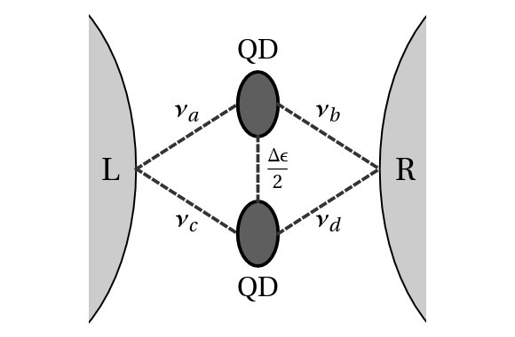
Figure 1: Schematic representation of the nanoelectronic device that is considered in the text. It consists of two quantum dots (QD) that are coupled with each other and to a left (L) and a right (R) electrode. In this work, the inter-dot coupling is assumed to be non-zero and smaller than the coupling to the leads, $0<\Delta\epsilon/2\ll\nu_{x}$, $x\in\{a,b,c,d\}$. Two cases of particular interest are coupling in a serial ($\nu_{a}=\nu_{d}\neq 0$, $\nu_{b}=\nu_{c}=0$) and a branched form ($\nu_{a}=\nu_{b}\neq 0$, $\nu_{c}=\nu_{d}=0$).

In this work, we identify the finite bandwidth of the leads as an important but previously poorly studied variable. Our detailed results show that it can induce a coupling between the eigenstates of the serial and branched realization or, equivalently, between the dots of a corresponding AB interferometer. This coupling gives rise to population inversion and a strong renormalization of the corresponding signatures in the transport characteristics, in particular an enhanced broadening. It is similar to Ruderman-Kittel-Kasuya-Yosida (RKKY) (spin-spin) interactions in solids Hewson (1993); Craig et al. (2004); Sasaki et al. (2006); Kulkarni and Konik (2011); Tutuc et al. (2011) and has also been referred to in the literature as an indirect coupling Kubo et al. (2008); Trocha (2012), where, however, it is associated with the fact that the two eigenstates/dots are coupled to the same leads rather than the energy dependence of the respective conduction bands.

Electron transport through such nanoelectronic devices has been studied using approximate methods like second Hettler et al. (2002, 2003); Muralidharan and Datta (2007); Darau et al. (2009); Härtle et al. (2009); Donarini et al. (2010); Härtle and Thoss (2011b) and higher order Pedersen and Wacker (2005); Pedersen et al. (2007); Leijnse and Wegewijs (2008); Esposito and Galperin (2010) master equation methodologies, real-time diagrammatic techniques König et al. (1996, 1996); Tews (2004); Wunsch et al. (2005), nonequilibrium Green’s function methods Meir et al. (1991); Groshev et al. (1991); Fransson (2005); Thygesen (2008); Bergfield and Stafford (2009); Härtle et al. (2009); Galperin et al. (2008); Roura-Bas et al. (2011) and (nonequilibrium) scattering state approaches Dutt et al. (2011). Numerically exact schemes based on time-convolutionless master equations Timm (2011), numerical Anders and Schiller (2005); Anders (2008); Korb et al. (2007) and functional Jakobs et al. (2007); Meden and Marquardt (2006) renormalization group theory Kashcheyevs et al. (2009), density matrix renormalization group methods Schmitteckert (2004); Pedersen et al. (2009); Heidrich-Meisner et al. (2009), flow equation approaches Kehrein (2005); Hackl et al. (2009); Eckstein et al. (2010), iterative Weiss et al. (2008); Segal et al. (2010); Hützen et al. (2012) and stochastic Werner et al. (2009); Schiró (2010); Han (2010); Mühlbacher et al. (2011); Gull et al. (2011) diagrammatic methods and wave-function propagation algorithms Wang and Thoss (2009, 2013) have also been used. Additionally, numerically exact reduced dynamics techniques, which exist for population dynamics Cohen and Rabani (2011) and transport properties, Cohen et al. (2013a) have been applied to both the stochastic diagrammatic methods Cohen et al. (2013b) and the wave function propagation schemes Wilner et al. (2013).

Our studies are based on the hierarchical quantum master equation (HQME) approach introduced by Jin et al. Jin et al. (2008) and modified by us in several ways, of which the most important is the use of a truncation scheme different from that proposed in Ref. Shi et al., 2009. The HQME method is in effect a perturbative expansion in powers of the dot-lead hybridization divided by the temperature; if carried to infinite order it is exact and if the temperature is not too low, convergence can be verified numerically. The advantages of the HQME method are that it is time-convolutionless, non-perturbative in the electron-electron interaction and gives numerically exact access to the steady state properties of nanoelectronic devices even in situations (such as those involving quasidegenerate levels Timm (2011)) where electronic relaxation time scales can become relatively long.

For comparison, we also employ two approximate methods: the Born-Markov (BM) master equation method May (2002); Hettler et al. (2002); Mitra et al. (2004); Lehmann et al. (2004); Harbola et al. (2006); Härtle et al. (2009); Härtle and Thoss (2011b) and a non-crossing approximation (NCA) calculation of the nonequilibrium Green’s function Keiter and Kimball (1970, 1971); Grewe and Keiter (1981); Kuramoto (1983); Coleman (1984); Bickers et al. (1987); Bickers (1987); Nordlander et al. (1999); Eckstein and Werner (2010); Gull et al. (2011). The comparison reveals the importance of a systematic (hybridization) expansion. In addition, it allows us to assess the role of renormalization and inter-state/inter-dot coupling effects arising from finite lead bandwidths (which is typically neglected) and the differences arising from different choices of lead density of states. Note that, only recently, the HQME framework was compared to master equation and nonequilibrium Greensfunction approaches in Ref. Popescu and Kleinekathöfer (2013), where simple (i.e. non-interacting) time-dependent transport problems were studied.

The article is organized as follows. In Sec. II, we outline the theoretical methodology, including a brief description of the spinless Anderson impurity model (Sec. II.1), the HQME approach (Sec. II.2), the BM master equation scheme (Sec. II.3) and the NCA based Green’s function scheme (Sec. II.4). Our results are presented in Sec. III, where we discuss the transport characteristics of the serial (Sec. III.1) and the branched (Sec. III.2) realizations of the spinless two-orbital Anderson model. On the single-particle level the parallel realization exhibits constructive interference. Here, the effect of (repulsive) electron-electron interactions can be readily understood as a blocking of transport channels in this system. In contrast, the serial conduction case shows pronounced destructive interference and decoherence induced phenomena which are analyzed in detail in Secs. III.1.1 – III.1.3. Sec. III.1.4 then examines the consequences of an asymmetric coupling to the electrodes while Sec. III.1.5 presents the gate-voltage dependence of the decoherence effects discussed here. A comparison to other systems which show negative differential resistance due to the effect of electron-electron interactions is given in Sec. III.1.6. In Sec. III.1.7, we consider the robustness of our conclusions under varying the lead density of states. Sec. III.1.8 includes a discussion of higher order effects and some numerical aspects.

II Theory

II.1 Model Hamiltonian

We consider interference effects in electron transport through a nanoelectronic system (S) that supports two quasidegenerate electronic states. A schematic is shown in Fig. 1. Physical realizations include two quantum dots arranged to form an Aharonov-Bohm interferometer Holleitner et al. (2001); Aikawa et al. (2004); Holleitner et al. (2002); Ihn et al. (2007) or a single nanoscale conductor with an appropriate level structure Kalyanaraman and Evans (2002); Ernzerhof et al. (2005); Solomon et al. (2008); Brisker-Klaiman and Peskin (2010); Markussen et al. (2010); Sparks et al. (2011); Brisker-Klaiman and Peskin (2012); Härtle and Thoss (2011a); Ballmann et al. (2012); Härtle et al. (2013a). We model this situation as a two orbital spinless Anderson model. The corresponding Hamiltonian reads

$$H_{\text{S}} = \epsilon_{1}d_{1}^{\dagger}d_{1}+\epsilon_{2}d_{2}^{\dagger}d_{2}+Ud_{1}^{\dagger}d_{1}d_{2}^{\dagger}d_{2},$$ (1)

where $U$ parametrizes the Coulomb interactions in this system.

The nanoelectronic system S is coupled to two macroscopic (metal) electrodes (L/R), which provide reservoirs of electrons. Departures from equilibrium may be achieved by choosing different chemical potentials or temperatures for the two leads. Each of the electrodes can be represented as a continuum of non-interacting electronic states

$$H_{\text{L/R}} = \sum_{k\in\text{L/R}}\epsilon_{k}c_{k}^{\dagger}c_{k}.$$ (2)

The coupling between the system S and the electrodes L and R is given by

$$H_{\text{tun}} = \sum_{k\in\text{L,R};m\in\{1,2\}}(V_{mk}c_{k}^{\dagger}d_{m}+\text{h.c.}).$$ (3)

The coupling matrix elements $V_{mk}$ determine the so-called level-width (or coupling density) functions

$$\Gamma_{K,mn}(\epsilon)=2\pi\sum_{k\in K}V_{mk}^{*}V_{nk}\delta(\epsilon-\epsilon_{k})$$ (4)

with $K\in\{\text{L,R}\}$. In the following, we assume these functions to be Lorentzian,

$$\Gamma_{K,mn}(\epsilon) = 2\pi\nu_{K,m}\nu_{K,n}\frac{\gamma}{(\epsilon-\mu_{K})^{2}+\gamma^{2}},$$ (5)

with the (band) width parameter $\gamma$, the chemical potential $\mu_{K}$ and $\nu_{K,m}$ denoting the coupling strength between state $m$ and lead $K$. This form of the level-width functions is advantageous in setting up the basic HQME framework. More general level-width functions can be implemented, using, for example, the Meir-Tannor parametrization scheme Meier and Tannor (1999); Welack et al. (2006); Jin et al. (2008). The basic physics that is discussed in this paper is not influenced by this choice of the level-width functions (cf. Sec. III.1.7).

We choose the zero of energy to be the average of the two lead chemical potentials and define $\Phi$ as the bias voltage, so the chemical potentials in the left and the right leads are given by $\mu_{\text{L}}=e\Phi/2$ and $\mu_{\text{R}}=-e\Phi/2$. This description is appropriate to devices with the structure of the quantum dot array in Fig. 1 and applies to physical realizations such as the Aharonov-Bohm-like setups of Refs. Ihn et al., 2007; Trocha et al., 2009; Bedkihal and Segal, 2012 as well as to most single-molecule junctions Datta et al. (1997); Mujica et al. (2002). Other geometries may require a different model for the drop of the bias voltage Fujisawa et al. (1998); Kießlich et al. (2007). The full Hamiltonian $H$ is given by

$$H = H_{\text{S}}+H_{\text{L}}+H_{\text{R}}+H_{\text{tun}}.$$ (6)

In the following, we assume the coupling strengths $\nu_{K,m}$ to be energy independent. While this is not the most general case, it provides a sufficient description of the condensed matter systems of main experimental interest. The assumption allows us to choose an energy independent basis where $\Gamma_{\text{L},mn}(\epsilon)\sim\delta_{m,1}\delta_{n,1}$ and $\Gamma_{\text{R},mn}(\epsilon)=0$ for $m,n>2$ and to separate the energy-dependent part of $\Gamma_{K,mn}(\epsilon)$, i.e. $2\pi\gamma/((\epsilon-\mu_{K})^{2}+\gamma^{2})$, from the part that depends on the degrees of freedom of the system S, $\nu_{K,m}\nu_{K,n}$. This allows us to significantly reduce the numerical effort in the HQME calculations described next.

II.2 Hierarchical master equation approach

To calculate the nonequilibrium transport properties of the spinless Anderson model, we use a modified version of the HQME method of Jin et al. Jin et al., 2008; Zheng et al., 2009. The approach is based on a representation of the reduced density matrix $\sigma$ in terms of the Feynman-Vernon influence functional Feynman and Vernon (1963); Makri and Makarov (1995); Segal et al. (2010). It was originally developed to describe bosonic reservoir degrees of freedom Tanimura and Kubo (1989); Tanimura (1990, 2006), which are important for example in photosynthesis Kreisbeck et al. (2011); Zhu and Kais (2011); Strümpfer and Schulten (2012). To lowest order, it reduces to the non-Markovian density matrix approach of Welack et al. Welack et al. (2006). The HQME framework is suitable for the present problem because it represents a time-convolutionless master equation approach Timm (2011) which allows us to address the long relaxation time scales in the presence of quasidegenerate levels and facilitates a non-perturbative description of electron-electron interactions. Moreover, populations and coherences of the system are treated on the same footing, which is necessary for the investigation of the complex interplay between interactions and quantum interference effects.

The central quantity of the approach is the reduced density matrix $\sigma(t)$. It is defined by the trace over the leads of the total density matrix $\varrho(t)$

$$\sigma(t) = \text{Tr}_{\text{L+R}}\left\{\varrho(t)\right\}.$$ (7)

The time dependence of the total density matrix $\varrho(t)$ can be written as

$$\varrho(t) = U(t,0)\varrho(0)U^{\dagger}(t,0)$$ (8)

with the time evolution operator

$$U(t,0) = T\left(\text{e}^{-i\int_{0}^{t}\text{d}\tau\left(H_{\text{tun}}(\tau)+H_{\text{S}}\right)}\right).$$ (9)

Here $T$ denotes the time ordering operator. Note that we have written the formalism in an interaction picture, where only the lead Hamiltonians $H_{\text{L/R}}$ are used but not the system Hamiltonian $H_{\text{S}}$. Thus, we avoid the direct appearance of dynamical phases in the reduced density matrix.

The equation of motion of the reduced density matrix is

$$\frac{\text{d}}{\text{d}t}\sigma(t) = -i\left[H_{\text{S}},\sigma(t)\right]-\sum_{m,s}\left[d_{m}^{s},\tilde{\sigma}_{ms}(t)\right].$$ (10)

with

$$\sum_{m,s}\left[d_{m}^{s},\tilde{\sigma}_{ms}(t)\right] = i\text{Tr}_{\text{L+R}}\left\{\left[H_{\text{tun}}(t),\varrho(t)\right]\right\}.$$ (11)

and $s\in\{+,-\}$, $d_{n}^{+}=d_{n}^{\dagger}$ and $d_{n}^{-}=d_{n}$. The reduced density matrix can thus be obtained from the operators $\tilde{\sigma}_{ms}(t)$. Writing equations of motion for these operators leads to an infinite hierarchy of equations involving the nested commutators $\left[H_{\text{tun}}(t),\left[H_{\text{tun}}(t),....,\varrho(t)\right]\right]$, $\left[\partial_{t}H_{\text{tun}}(t),\left[H_{\text{tun}}(t),....,\varrho(t)\right]\right]$ and so on. In practical calculations, this set of equations needs to be truncated at some finite level. However, it is not a priori clear which of these operators can be neglected; in particular, a systematic method for dropping operators involving the time derivatives $\partial_{t}^{q}H_{\text{tun}}(t)$ with $q\in\mathbb{N}$ seems not to be available.

The HQME approach of Jin et al. Jin et al. (2008) solves this problem in two steps. First, the operators $\tilde{\sigma}_{ms}(t)$ are rewritten as

$$\tilde{\sigma}_{ms}(t) = \sum_{Kn}\int_{0}^{t}\text{d}\tau\,C^{\overline{s}}_{K,mn}(t-\tau)\text{Tr}_{\text{L+R}}\left\{U(t,\tau)d_{n}^{\overline{s}}U(\tau,0)\varrho(0)U^{\dagger}(t,0)\right\}$$

$$-\sum_{Kn}\int_{0}^{t}\text{d}\tau\,C^{s,*}_{K,mn}(t-\tau)\text{Tr}_{\text{L+R}}\left\{U(t,0)\varrho(0)U^{\dagger}(\tau,0)d_{n}^{\overline{s}}U^{\dagger}(t,\tau)\right\},$$

using the correlation functions

$$C^{s}_{K,mn}(t-t^{\prime}) = \sum_{k\in K}V^{\overline{s}}_{mk}V_{nk}^{s}\text{Tr}_{K}\left\{\sigma_{K}c_{k}^{s}(t)c_{k}^{\overline{s}}(t^{\prime})\right\},$$ (13)

where

$$\sigma_{K} = \frac{1}{\text{Tr}_{K}\left\{\text{e}^{-\sum_{k\in K}\frac{\epsilon_{k}-\mu_{\text{L/R}}}{k_{\text{B}}T}c_{k}^{\dagger}c_{k}}\right\}}\text{e}^{-\sum_{k\in K}\frac{\epsilon_{k}-\mu_{\text{L/R}}}{k_{\text{B}}T}c_{k}^{\dagger}c_{k}},$$ (14)

$k_{\text{B}}$ denotes the Boltzmann constant, $T$ the temperature of the electrodes, $\overline{s}=-s$, $V_{mk}^{+}=V_{mk}$, $V_{mk}^{-}=V_{mk}^{*}$, $c_{k}^{+}=c_{k}^{\dagger}$ and $c_{k}^{-}=c_{k}$. Note that in deriving these expressions it has been assumed that the system is initially in a factorized state, i.e. that the density matrix $\varrho(0)$ at time $t=0$ is given by the product $\sigma(0)\sigma_{\text{L}}\sigma_{\text{R}}$. This choice of the initial state is not important in the present context, because we wish to study the steady state properties of the system S.

Second, the correlation functions $C^{s}_{K,mn}$ are represented by a set of exponential functions,

$$C^{s}_{K,mn}(t) = \frac{\nu_{K,m}\nu_{K,n}}{\gamma}\sum_{p\in\mathbb{N}_{0}}\eta^{s}_{K,p}\text{e}^{-\omega^{s}_{K,p}t}.$$ (15)

which, due to the self similarity of these exponentials with respect to time derivatives, i.e. $\partial_{t}\text{exp}(-\omega t)\sim\text{exp}(-\omega t)$, can also be used to represent the respective time derivative, $\partial_{t}C^{s}_{K,mn}(t)$. This property is crucial because it will allow us to express the various time derivatives of the hybridization operator $H_{\text{tun}}(t)$, which appeared before in the nested commutators $\left[H_{\text{tun}}(t),\left[H_{\text{tun}}(t),....,\varrho(t)\right]\right]$, $\left[\partial_{t}H_{\text{tun}}(t),\left[H_{\text{tun}}(t),....,\varrho(t)\right]\right]$ and so on, in terms of known auxiliary operators rather than an infinite series of unknown ones and, thus, to truncate the corresponding equations of motion in a systematic way (vide infra). Explicitly,

$$\omega^{\pm}_{K,p} = \left\{\begin{array}[]{ll}\gamma\mp i\mu_{K},&p=0,\\ \pi k_{\text{B}}T(2p-1)\mp i\mu_{K},&p\in\mathbb{N},\\ \end{array}\right.$$ (18)

$$\eta^{\pm}_{K,p} = \left\{\begin{array}[]{ll}\pi\frac{\gamma}{1+\text{exp}(i\frac{\gamma}{k_{\text{B}}T})},&p=0,\\ -2\pi ik_{\text{B}}T\frac{\gamma^{2}}{(\mu_{K}\mp i\omega_{K,p}^{\pm})^{2}+\gamma^{2}},&p\in\mathbb{N},\\ \end{array}\right.$$ (21)

where contour integration has been used to obtain the final result. This representation relies on the assumption that the level-width function $\Gamma_{K,mn}$ can be represented by a set of Lorentzians (cf. Eq. 5). The operators $\tilde{\sigma}_{ms}(t)$ can thus be expressed in terms of a new class of auxiliary operators

$$\sigma_{K,n,s,p}(t) = \eta^{s}_{K,p}\int_{0}^{t}\text{d}\tau\,\text{e}^{-\omega^{s}_{K,p}(t-\tau)}\text{Tr}_{\text{L+R}}\left\{U(t,\tau)d_{n}^{s}U(\tau,0)\varrho(0)U^{\dagger}(t,0)\right\}$$

$$-\eta^{\overline{s},*}_{K,p}\int_{0}^{t}\text{d}\tau\,\text{e}^{-\omega^{s}_{K,p}(t-\tau)}\text{Tr}_{\text{L+R}}\left\{U(t,0)\varrho(0)U^{\dagger}(\tau,0)d_{n}^{s}U^{\dagger}(t,\tau)\right\}$$

as

$$\tilde{\sigma}_{ms}(t) = \sum_{Knp}\frac{\nu_{K,m}\nu_{K,n}}{\gamma}\sigma_{K,n,\overline{s},p}(t).$$ (23)

Note that, in general, a decomposition in terms of exponential functions is only possible for non-zero temperatures. At $T=0$ correlation functions $C^{s}_{K,mn}$ may, in general, exhibit a $1/t$ dependence, which cannot be represented by a set of exponentials.

The equations of motion of the auxiliary operators $\sigma_{K,n,s,p}(t)$ represent the first tier of an infinite hierarchy of equations of motion Jin et al. (2008). The full hierarchy is then written as

$$\partial_{t}\sigma^{(\alpha)}_{j_{1}..j_{\alpha}}(t) = -i\left[H_{\text{S}},\sigma^{(\alpha)}_{j_{1}..j_{\alpha}}(t)\right]-\sum_{\beta\in\{1..\alpha\}}\omega_{K_{\beta},p_{\beta}}^{s_{\beta}}\sigma^{(\alpha)}_{j_{1}..j_{\alpha}}(t)$$

$$+\sum_{\beta\in\{1..\alpha\}}(-1)^{\alpha-\beta}\eta_{K_{\beta},p_{\beta}}^{s_{\beta}}d_{m_{\beta}}^{s_{\beta}}\sigma^{(\alpha-1)}_{j_{1}..j_{\alpha}/j_{\beta}}(t)+\sum_{\beta\in\{1..\alpha\}}(-1)^{\beta}\eta_{K_{\beta},p_{\beta}}^{\overline{s}_{\beta},*}\sigma^{(\alpha-1)}_{j_{1}..j_{\alpha}/j_{\beta}}(t)d_{m_{\beta}}^{s_{\beta}}$$

$$-\sum_{j_{\alpha+1},n_{\alpha+1}}\frac{\nu_{K_{\alpha+1},m_{\alpha+1}}\nu_{K_{\alpha+1},n_{\alpha+1}}}{\gamma}\left(d_{n_{\alpha+1}}^{\overline{s}_{\alpha+1}}\sigma^{(\alpha+1)}_{j_{1}..j_{\alpha}j_{\alpha+1}}(t)-(-1)^{\alpha}\sigma^{(\alpha+1)}_{j_{1}..j_{\alpha}j_{\alpha+1}}(t)d_{n_{\alpha+1}}^{\overline{s}_{\alpha+1}}\right),$$

where the reduced density matrix and the auxiliary operators enter as $\sigma^{(0)}(t)=\sigma(t)$ and $\sigma^{(1)}_{j_{1}}(t)=\sigma_{K,n,s,p}(t)$, using superindices $j_{\beta}=(K_{\beta},m_{\beta},s_{\beta},p_{\beta})$ for notational reasons ($\alpha,\beta\in\mathbb{N}$). The higher tier operators $\sigma^{(\alpha)}_{j_{1}..j_{\alpha}}(t)$ ($\alpha\geq 2$) are associated with the nested commutators $\left[H_{\text{tun}}(t),\left[H_{\text{tun}}(t),....,\varrho(t)\right]\right]$. They can be represented by a set of superoperators, which are defined by

$$B_{j}\varrho(t) \equiv \sigma^{(1)}_{j_{1}}(t),$$ (25)

as

$$\sigma^{(\alpha+1)}_{j_{1}..j_{\alpha+1}}(t) = B_{j_{\alpha}}..B_{j_{1}}\varrho(t).$$ (26)

They enter the hierarchy (II.2) with prefactors $\nu_{K_{\alpha+1},m_{\alpha+1}}\nu_{K_{\alpha+1},n_{\alpha+1}}/\gamma$ such that a truncation of the hierarchy at the $\alpha$th tier leads to an equation of motion for the reduced density matrix that is valid up to the $\alpha$th order in the hybridization strength $\varGamma=\text{max}(\nu_{K,m}\nu_{K,n}/\gamma)$. The corresponding dimensionless expansion parameter is the ratio of $\varGamma$ to the minimal value of $\text{Re}\left[\omega^{\pm}_{K,p}\right]$, which is $\sim\text{min}(\gamma,k_{\text{B}}T)$. Thus, for example, the approach can be expected to describe Kondo physics if the ratio $\varGamma/(k_{\text{B}}T_{\text{Kondo}})$ of the hybridization strength and the Kondo temperature is smaller or comparable to one (although convergence may be achieved for larger values as well) Zheng et al. (2009); Li et al. (2012). Further details on how the hierarchy of equations of motion (II.2) is solved numerically are given in App. A.

While our approach closely follows that of Jin et al. Jin et al. (2008) we redefined the auxiliary operators (cf. Eq. II.2) in a dimensionless way and formulated an improved measure for truncating the hierarchy of equations of motion systematically (see App. A). Thereby, in contrast to earlier work Shi et al. (2009), our methodology respects the internal structure of both the auxiliary operators and the corresponding equations of motion. Moreover, our choice of the level-width functions (cf. Eq. 5) means that, by working in a basis where $\Gamma_{\text{L},mn}(\epsilon)\sim\delta_{m,1}\delta_{n,1}$ and $\Gamma_{\text{R},mn}(\epsilon)=0$ for $m,n>2$, the state variables $m_{\beta}$ and $n_{\beta}$ become redundant. In the present context, this reduces the number of superindices from $2\cdot N_{\text{leads}}\cdot N_{\text{el}}^{2}\cdot N_{p}$ to $2\cdot(N_{\text{leads}}+1)\cdot N_{p}$, where $N_{\text{leads}}$, $N_{\text{el}}$ and $N_{p}$ denote the number of electrodes, eigenstates of the system $S$ and the number of terms considered in the decomposition (15), respectively.

In addition to the Matsubara decomposition (15), other schemes are based on, for example, Gauss-Legendre or Gauss-Chebyshev quadrature schemes of the Fourier transforms of $C^{s}_{K,mn}(t)$ Heng and Chen (2012), or on hybrid schemes of the latter and the Matsubara decomposition scheme Zheng et al. (2009) or on Pade approximation schemes Ozaki (2007); Hu et al. (2010, 2011). Thus, the efficiency of the HQME method can be somewhat increased (see the discussion at the end of Sec. III.1.8). However, the basic methodological characteristics, in particular that the method is in effect an expansion in $\varGamma/\text{min}(\gamma,k_{\text{B}}T)$, are maintained. Further theoretical progress is required to address the moderate to strong coupling regime, where the hybridization is comparable to or larger than the temperature scales of the system (such as, e.g., deep inside the Kondo regime).

II.3 Born-Markov master equation approach

The long-time limit of the reduced density matrix $\sigma$ is often approximated as the stationary solution of the well-established equation of motion May (2002); Mitra et al. (2004); Lehmann et al. (2004); Harbola et al. (2006); Volkovich et al. (2008); Härtle et al. (2009, 2010); Härtle and Thoss (2011b)

$$\frac{\partial\sigma(t)}{\partial t} = -i\left[H_{\text{S}},\sigma(t)\right]-\int_{0}^{\infty}\text{d}\tau\,\text{tr}_{\text{L+R}}\{\left[H_{\text{tun}},\left[\tilde{H}_{\text{tun}}(\tau),\sigma(t)\sigma_{\text{L+R}}\right]\right]\},$$ (27)

with

$$\tilde{H}_{\text{tun}}(\tau)=\text{e}^{-i(H_{\text{S}}+H_{\text{L}}+H_{\text{R}})\tau}H_{\text{tun}}\text{e}^{i(H_{\text{S}}+H_{\text{L}}+H_{\text{R}})\tau}.$$ (28)

Here, $\sigma_{\text{L+R}}$ represents the equilibrium density matrix of the leads. Eq. (27) can be derived from the Nakajima-Zwanzig equation Nakajima (1958); Zwanzig (1960), employing a second-order expansion in the coupling $H_{\text{tun}}$ along with the so-called Markov approximation. Note that the master equation (27) corresponds to the Redfield (or Bloch-Wangsness-Redfield) equation if it is evaluated in the eigenbasis of the system Hamiltonian $H_{\text{S}}$ Wangsness and Bloch (1953); Redfield (1965); May and Kühn (2004).

The BM master equation (27) is commonly evaluated by neglecting the real part $\mathbf{\Delta}$ of the self-energy matrix $\mathbf{\Sigma}=\mathbf{\Delta}-(i/2)\mathbf{\Gamma}$, which is associated with the coupling between the system S and the electrodes L and R. Thus, the renormalization of the energy levels 1 and 2 due to the coupling to the leads (given by the diagonal elements $\Delta_{11}$ and $\Delta_{22}$ Harbola et al. (2006); Härtle and Thoss (2011b)) is neglected. A coupling between these states mediated by the off-diagonal elements $\Delta_{12}$ is also neglected. For systems without quasidegenerate levels, these terms are not important Härtle and Thoss (2011b) but in the present situation we will see by comparison to the HQME method (vide infra) that this inter-state coupling can play an important role for the transport properties.

II.4 Nonequilibrium Green’s function approach based on the non-crossing approximation

The NCA is a popular and successful method for calculating the nonequilibrium Green’s functions of quantum dotsKeiter and Kimball (1970, 1971); Grewe and Keiter (1981); Kuramoto (1983); Coleman (1984); Bickers et al. (1987); Bickers (1987); Nordlander et al. (1999); Eckstein and Werner (2010); Gull et al. (2011). The NCA involves a hybridization expansion, where non-crossing diagrams of all orders are summed in terms of a Dyson series, but diagrams with crossing hybridization lines are excluded. As an approximate method, it should always be considered less reliable than converged numerically exact results like HQME and quantum Monte Carlo schemes Gull et al. (2011); Eckstein and Werner (2010); Cohen et al. (2013a). Nevertheless, the NCA can capture qualitative aspects of the physics involved in this problem and represents a standard methodology for the description of electron-electron interaction effects. It is thus very useful to compare exact results obtained with HQME to the ones obtained with NCA. In the present context, the simplicity and flexibility of the NCA even facilitates a study of the effects for different lead density of states (see Sec. III.1.7).

In order to extend the NCA framework to the spinless Anderson model, we consider the Dyson equation for the causal propagator $G\left(t\right)=\mathrm{Tr}_{\text{L+R}}\left\{\rho\left(t=0\right)e^{-iHt}\right\}$:

$$G\left(t-t^{\prime}\right)=G^{\left(0\right)}\left(t-t^{\prime}\right)+\int_{t^{\prime}}^{t}\mathrm{d}t_{1}\int_{t^{\prime}}^{t1}\mathrm{d}t_{2}G^{\left(0\right)}\left(t-t_{1}\right)\Sigma\left(t_{1},t_{2}\right)G\left(t_{2}-t^{\prime}\right).$$ (29)

Here, $G^{\left(0\right)}$ is the propagator for the case where the dot-lead coupling is set to zero and the self-energy $\Sigma$ induces all diagrams arising from the coupling to the electrodes. The matrix elements $G_{ab}\equiv\left\langle a\right|G\left|b\right\rangle$ of the propagator in the basis of the dot states can be conveniently represented by a pair of lines (one for the occupation of each spin level, cf. Fig. 2), where a dashed line stands for an empty level and a solid line for a full one.

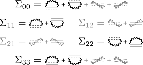
Figure 2: NCA self-energy diagrams for the spinless Anderson model; gray terms are identically zero in the regular Anderson model.

In the spinful Anderson model, $G$ is diagonal in this basis and pairs of interactions with the electrodes can be represented diagrammatically as wavy lines which flip one spin between interactions (when using the shorthand diagrams in which the many-body state on the dot is represented by a single line, the sum over the two arcs is often compactly represented by a single one). The definition of the NCA self-energy is then given by the black diagrams in Fig. 2.

The new feature of the model we consider is that non-diagonal ($m\neq n$) contributions to $\Gamma_{K,mn}(\epsilon)$ are also present. These induce a new kind of hybridization line, which takes an electron from one level to the other. The additional diagrams are shown in gray in Fig. 2; note that, as a result, $G_{ab}$ for $\left|a\right\rangle=\left|01\right\rangle,\,\left|b\right\rangle=\left|10\right\rangle$ and vice-versa become non-zero and are represented by pairs of lines in which the level occupations trade places. The need to store and compute additional matrix-elements in the spinless case complicates the calculation somewhat, but no conceptual differences arise. Similar NCA treatments have been used to study multi-orbital models Korytár and Lorente (2011); Korytár et al. (2012) and the spinless Anderson model Roura Bas and Aligia (2010); Roura-Bas et al. (2011); Trocha (2012). However, it is important to note that what the authors of these works refer to as the NCA is an infinite-$U$ approach which differs from the finite-$U$ method employed here.

II.5 Observables of interest

The crucial quantities that characterize the nonequilibrium transport properties of interest here are the steady state level populations $n_{1/2}$, the inter-level coherence $\sigma_{10,01}$ and the electrical current that is flowing through the system S. In the occupation number representation, the population of the electronic levels is given by the diagonal elements of the reduced density matrix

$$n_{1} = \lim_{t\rightarrow\infty}\left(\sigma_{10,10}(t)+\sigma_{11,11}(t)\right),$$ (30)

$$n_{2} = \lim_{t\rightarrow\infty}\left(\sigma_{01,01}(t)+\sigma_{11,11}(t)\right),$$ (31)

while the off-diagonal elements of the reduced density matrix determine the coherence

$$\sigma_{10,01} = \lim_{t\rightarrow\infty}\sigma_{10,01}(t).$$ (32)

The coherence has no classical analog; it encodes quantum mechanical tunneling and interference effects. For well separated energy levels, coherences of the density matrix vanish. For degenerate or quasidegenerate levels, however, coherences can become as important as the populations $n_{1/2}$. In the present context, the inter-level coherence can be used as a measure for the strength of interference effects, that is comparison of the coherence found in the interacting and non-interacting situations provides an assessment of the importance of interaction-induced decoherence.

The electrical current flowing through the systems S is determined by the number of electrons that enter or leave the electrode $K$ in a given interval of time ($K\in\{\text{L,R}\}$)

$$I_{K} = -e\frac{\text{d}}{\text{d}t}\sum_{k\in K}\langle c^{\dagger}_{k}c_{k}\rangle\equiv\langle\hat{I}_{K}\rangle,$$ (33)

where $-e$ denotes the charge of an electron. It can be written in terms of the first-tier auxiliary operators $\sigma^{(1)}_{j}(t)$ as Jin et al. (2008)

$$I_{K} = e\sum_{K,m,n,p}\frac{\nu_{K,m}\nu_{K,n}}{\gamma}\lim_{t\rightarrow\infty}\left(\text{Tr}_{\text{S}}\left[\sigma_{K,m,+,p}(t)d_{n}\right]-\text{Tr}_{\text{S}}\left[d_{n}^{\dagger}\sigma_{K,m,-,p}(t)\right]\right).$$ (34)

or, using the BM master equation scheme (see Sec. II.3), as

$$I_{K} = -i\lim_{t\rightarrow\infty}\int_{0}^{\infty}\text{d}\tau\,\text{tr}\{\left[\tilde{H}_{\text{tun}}(\tau),\sigma_{\text{L+R}}\sigma(t)\right]\hat{I}_{K}\}.$$ (35)

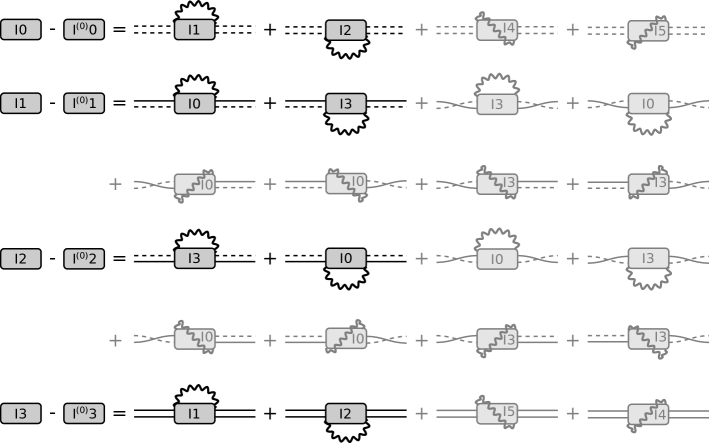
Figure 3: NCA diagonal vertex diagrams for the spinless Anderson model; gray terms are identically zero in the regular Anderson model.

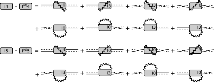
Figure 4: NCA off-diagonal vertex diagrams for the spinless Anderson model; all the terms appearing here are identically zero in the regular Anderson model.

The computation of the electronic state populations, the coherence and the electrical current within the NCA framework requires the solution of a set of secondary vertex equations. A vertex is defined in this context as an object which exists on both parts of the contour simultaneously (cf. Figs. 3 and 4). It is specified by an inner vertex, which is associated with the corresponding observable (for instance, the inner vertex corresponding to measuring the population in the state $\left|a\right\rangle$ is given by $P_{ab}\left(t,t^{\prime}\right)=G_{aa}\left(t\right)G_{aa}^{\dagger}\left(t^{\prime}\right)\delta_{ab}$) and outer indices, which connect the inner vertex to the initial state of the system via the propagator (29). Together with the specification of the observable, the vertex equations form a set of coupled integral equations which when solved together provide a self-consistent resummation of all contour-crossing NCA diagrams. The vertex terms which appear in the original Anderson case are the dark diagrams in Fig. 3; off-diagonal vertex contributions are unique to the spinless case and shown in Fig. 4. An alternative scheme, formulated in terms of correlation functions instead of propagators, has been proposed Eckstein and Werner (2010) but will not be used here.

III Results

We study two complementary realizations of the spinless Anderson model, which we refer to as DES and CON. The DES realization may represent a linear (molecular) conductor Solomon et al. (2008); Härtle et al. (2013a) or two quantum dots connected in series. The second system, model CON, may represent a branched (molecular) conductor Brisker et al. (2008); Härtle et al. (2013a) or two quantum dots connected in parallel Holleitner et al. (2001, 2002); Aikawa et al. (2004); König and Gefen (2002); Kubala and König (2002); Cohen et al. (2007); Ihn et al. (2007); Bedkihal and Segal (2012). Mathematically the two models are distinguished by the coupling parameters, which reflect the different connectivities of the eigenstates and the leads. In model DES these coupling parameters are symmetric, $\nu_{\text{L},1}=\nu_{\text{R},1}$, and antisymmetric, $\nu_{\text{L},2}=-\nu_{\text{R},2}$, respectively (the corresponding dot-lead coupling parameters (cf. Fig. 1) are $\nu_{a/d}=\sqrt{\nu_{\text{L/R},1}^{2}+\nu_{\text{L/R},2}^{2}}$ and $\nu_{b/c}=0$). On the single-particle level it has been shown that this form of the coupling produces strong destructive interference effects which suppress the current flow Härtle et al. (2011, 2013a). In model CON the coupling parameters $\nu_{K,1/2}$ are the same or, equivalently, symmetric ($\nu_{a/b}=\sqrt{\nu_{\text{L/R},1}^{2}+\nu_{\text{L/R},2}^{2}}$ and $\nu_{c/d}=0$). Thus, the system shows constructive interference effects . A detailed list of model parameters is given in Tab. 1. Note that these model parameters reflect typical experimental values Holleitner et al. (2001); Ihn et al. (2007); Osorio et al. (2007); Nilsson et al. (2010) with respect to the temperature scale $k_{\text{B}}T\approx 25$ meV that is used in this article.

	model			$\epsilon_{1}$			$\epsilon_{2}$			$U$			$\nu_{\text{L},1}$			$\nu_{\text{L},2}$			$\nu_{\text{R},1}$			$\nu_{\text{R},2}$			$\gamma$
	DES			0.5			0.501			0.5			$\nu$			$\nu$			$-\nu$			$\nu$			2
	CON			0.5			0.501			0.5			$\nu$			$\nu$			$\nu$			$\nu$			2
	CENTRAL			0.5			0.75			0.5			$\nu$			$\nu$			$\nu/3$			$\nu/3$			2
	BLOCK			0.5			0.75			0.5			$\nu$			$\nu$			$\nu$			$\nu/3$			2

Table 1: Parameters for the double dot devices that are investigated in this article. All energy values are given in $\mathrm{eV}$, the temperature of the electrodes $T$ is set to $300$ K ($\simeq 25$ meV) and the value of the dot-lead coupling parameter is $\nu=42$ meV.

III.1 Transport properties of junction DES

The calculated current-voltage characteristic of junction DES is shown as the solid blue line in Fig. 5a. The current increases monotonically with bias voltage $\Phi$ for $\Phi\lesssim 1.7$ V. The monotonic increase occurs both in the non-resonant transport regime ($0<e\Phi\lesssim 2\epsilon_{1/2}\approx 1$ eV), where both eigenstates of the junction are located outside the bias window, i.e. $\epsilon_{1/2}>\mu_{K}$, and in part of the resonant transport regime ($2\epsilon_{1/2}\lesssim e\Phi\lesssim 2\epsilon_{1/2}+U\approx 1.5$ eV) where the two levels are located within the bias window, i.e. $\mu_{\text{L}}>\epsilon_{1/2}>\mu_{\text{R}}$. As the voltage is increased beyond $\Phi\approx 1.7$ V, junction DES shows a voltage range with a pronounced decrease of the electrical current as voltage is increased, in other words a negative differential resistance which for the parameters considered here is peaked at $\Phi\approx 1.9$ V.

(a)

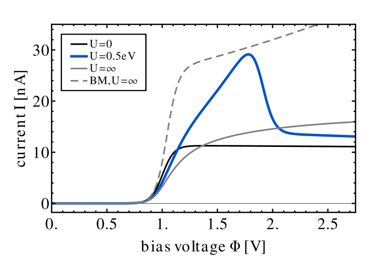
(b)

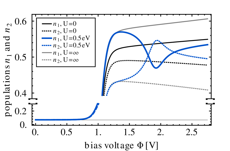
Figure 5: (Color online) Current-voltage and electronic population characteristics of junction DES calculated for different electron-electron interaction strengths: $U=0$ (black lines), $U=\infty$ (gray lines) and $U\approx 20k_{\text{B}}T$ (blue lines). The solid lines have been obtained using the HQME method. The dashed line has been computed with the BM scheme. Negative differential resistance occurs in the same voltage range where an inversion of the electronic populations $n_{1}$ (solid lines) and $n_{2}$ (dotted lines) occurs.

The corresponding populations of the electronic levels $n_{1}$ and $n_{2}$ are shown as the solid and dotted blue lines in Fig. 5b, respectively. The two levels are almost unpopulated in the non-resonant transport regime. In the resonant transport regime, the chemical potential in one of the leads exceeds the level positions and, accordingly, the population of the two levels increases substantially such that the average number of electrons in the junction is close to $n_{1}+n_{2}\approx 1$. Despite the near degeneracy of the two levels, their populations differ significantly. Moreover, an inversion of the population occurs for the bias voltages where the decrease of the current level is most pronounced.

We now show that this behavior is associated with the quenching of destructive interference effects due to electron-electron interactions and the energy-dependence of the density of states in the electrodes. The argument has three steps. First, we study the case where no electron-electron interactions are present in the system ($U=0$) and destructive interference effects are fully developed. Second, we consider the limit $U\rightarrow\infty$, where destructive interference effects appear to be quenched. In the third and final step, we consider a finite value for $U$ and show that the quenching of interference effects due to electron-electron interactions is no longer effective once the bias voltage exceeds $\approx 2(\epsilon_{1/2}+U)$.

III.1.1 The non-interacting limit

If electron-electron interactions are neglected in model DES, one obtains the current-voltage characteristic represented by the solid black line in Fig. 5a. It shows a single step at $e\Phi\approx 2\epsilon_{1/2}$ that indicates the onset of resonant transport through states 1 and 2. The low value of the current is due to destructive interference effects Solomon et al. (2008); Härtle et al. (2013a). This can be inferred from an analysis in terms of a BM master equation scheme (cf. Sec. II.3) May (2002); Mitra et al. (2004); Harbola et al. (2006); Härtle and Thoss (2011b). Using Eqs. A1 and A4 of Ref. Härtle and Thoss (2011b), the current through junction DES can be written as

$$I = 2e\Gamma\left(\sigma_{10,10}+\sigma_{10,10}-2\text{Re}\left[\sigma_{10,01}\right]\right),$$ (36)

where $\Phi>2\epsilon_{1/2}$ is assumed and the wide-band approximation with $\Gamma=\Gamma_{\text{L},11}(\mu_{\text{L}})$ is employed. The first two terms are given by the population of the singly occupied states $\sigma_{10,10}$ and $\sigma_{10,10}$, respectively. They represent the incoherent sum current that is flowing through the two states and are approximately given by the sum of the populations $n_{1}+n_{2}\approx\sigma_{10,10}+\sigma_{10,10}$. In the resonant transport regime, this sum is $\approx 1$, indicating that the bottleneck for transport is given by the small inter-dot coupling $(\epsilon_{2}-\epsilon_{1})/2$ rather than by the coupling to the electrodes (i.e. the system S is mostly occupied by a single electron). The last term is given by the real part of the coherence $\sigma_{10,01}$. It encodes the effect of destructive interference and is depicted in Fig. 6. As can be seen, it almost cancels the first two terms, since its value is very close to $0.5$ in the resonant transport regime. The real part of the coherence $\sigma_{10,01}$ can thus be used as a measure for the strength of destructive interference.

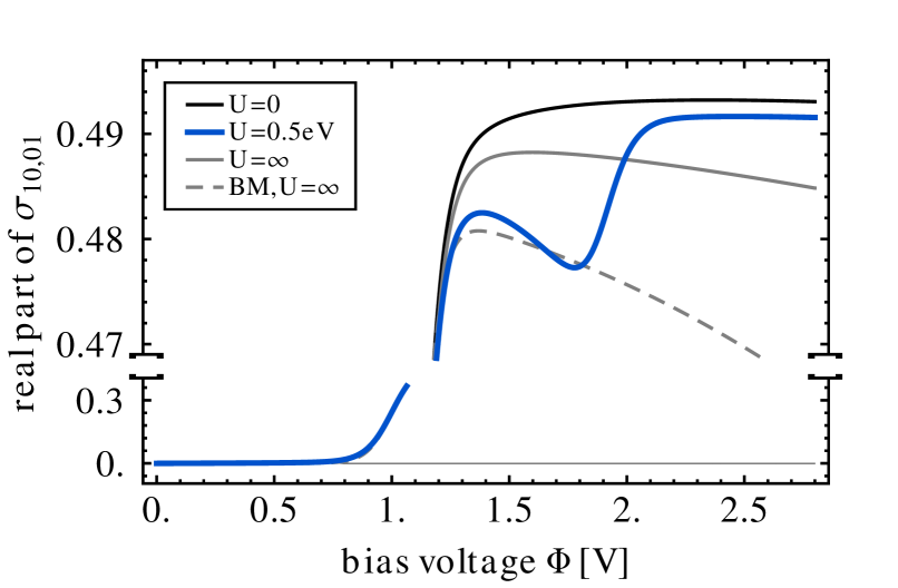
Figure 6: (Color online) Real part of the coherence $\sigma_{10,01}$ corresponding to the characteristics shown in Fig. 5. Comparison to the non-interacting case (black line) quantifies the effect of decoherence due to electron-electron interactions.

While the suppression of the current flow in systems like junction DES is well known Solomon et al. (2008); Härtle et al. (2013a), it is less recognized that in this model the population of the electronic levels is significantly different. The two level occupancies are depicted in Fig. 5b by the solid black and the dotted black line, respectively. The voltage dependence of the level occupancies is in general similar to that of the corresponding current-voltage characteristic, in particular exhibiting a step at $e\Phi\approx 2\epsilon_{1/2}$. Despite the near degeneracy of the level energies, the corresponding populations are not the same, where, for voltages larger than $e\Phi\approx 2\epsilon_{1/2}$, the population difference even increases with the applied bias voltage.

An analysis of the retarded/advanced single-particle Green’s functions $G^{\text{r/a}}_{mn}(\epsilon)$ reveals the origin of this behavior. They are defined by Haug and Jauho (1996)

$$\textbf{G}^{\text{r/a},-1}_{mn}(\epsilon) = (\epsilon-\epsilon_{m})\delta_{mn}-\Delta_{K,mn}(\epsilon)+\frac{i}{2}\Gamma_{K,mn}(\epsilon).$$ (37)

Thereby, the functions $\Delta_{K,mm}(\epsilon)$ denote the renormalization of the energy levels $\epsilon_{m}$ due to the coupling of the junction to lead $K$ and the off-diagonal elements $\Delta_{K,mn}(\epsilon)$ ($m\neq n$) encode a inter-state coupling which is induced by the energy dependence of $\Gamma_{K,12}(\epsilon)$. In the present context, the energy dependence is due to the finite bandwidth $\gamma$. In general, it may also be the result of an energy dependence of the couplings $\nu_{K,m}$. Using the Green’s functions $\textbf{G}^{\text{r/a}}_{mn}(\epsilon)$, the population of the two levels can be calculated according to the formula

$$n_{m} = \int\frac{\text{d}\epsilon}{2\pi}\sum_{Kno}G^{\text{r}}_{mn}(\epsilon)\Gamma_{K,no}(\epsilon)G^{\text{a}}_{om}(\epsilon)f_{K}(\epsilon).$$ (38)

This procedure yields exactly the same result as the one that is obtained by the HQME method outlined in Sec. II.2. However, if the off-diagonal elements $\Delta_{K,12}(\epsilon)$ are neglected , the populations of the two levels become very similar ($n_{1}-n_{2}<10^{-3}$ for $\Phi>2\epsilon_{12}+k_{\text{B}}T$). This shows that the off-diagonal elements $\Delta_{K,12}(\epsilon)$ cause the pronounced asymmetry in the electronic populations $n_{1}$ and $n_{2}$ . Note that Eq. (36) is derived from Born-Markov theory, where the effect of the off-diagonal elements $\Delta_{K,12}(\epsilon)$ is neglected such that the corresponding difference in the electronic populations $n_{1}$ and $n_{2}$ is small, that is the relation $I>2e\Gamma\sqrt{|n_{1}-n_{2}|}$ (which can be derived using the relation $|\rho_{10,01}|<\sqrt{\rho_{10,10}\rho_{01,01}}$) is fullfilled.

III.1.2 Decoherence phenomena in the limit $U\rightarrow\infty$

Now, we consider junction DES in the limit $U\rightarrow\infty$. The gray lines in Fig. 5b show the corresponding electronic populations $n_{1}$ (solid) and $n_{2}$ (dotted). The difference in the electronic populations is seen to be considerably larger at $U=\infty$ than it is at $U=0$. The $U$-dependence arises because, at $U=\infty$, transport through one of the two levels is completely blocked whenever the other level is occupied.

The current-voltage characteristic at $U=\infty$ is shown as the solid gray line in Fig. 5a. At $U=\infty$ the current is smaller than the $U=0$ current at low and intermediate bias voltages, i.e. for $\Phi<1.3$ V, but is larger for higher bias voltages and continues to increase as $\Phi$ is increased further into the resonant transport regime. The increase of the current is accompanied by a decrease of the real part of the coherence $\sigma_{10,01}$ (compare the solid gray and black lines in Fig. 6), indicating that the quenching of destructive interference effects, which are suppressing the current flow in this system, becomes progressively stronger as the voltage is increased.

This decoherence effect can be qualitatively understood via a Born-Markov analysis similar to that previously given for the non-interacting case (cf. Eq. 36). In the limit $U\rightarrow\infty$ and in the Born-Markov approximation, the current is given by

$$I = e\Gamma\left(\sigma_{10,10}+\sigma_{10,10}-2\text{Re}\left[\sigma_{10,01}\right]\right).$$ (39)

Comparison to Eq. (36) shows that within the BM approximation the $U=\infty$ current is a factor of two smaller than the $U=0$ current. However, a decrease in the real part of the coherence $\sigma_{10,01}$ overrides this effect, so that the net result is an enhancement of the current (cf. Figs. 5a and 6). The difference with respect to the non-interacting case arises from the reduction of the Hilbert space of the system S in the limit $U\rightarrow\infty$; this influences the scattering phase shift of the tunneling electrons and quenches interference effects in this system due to a reduction of interfering tunneling pathways.

This change in the scattering phase shift has already been discussed by Wunsch et al. Wunsch et al. (2005) in terms of an interaction-induced renormalization of the (localized) orbitals (and was also found in more complex systems Darau et al. (2009); Donarini et al. (2010)). These results, however, have been derived assuming flat conduction bands, where additional renormalization effects due to the energy dependence of the conduction bands are not present. Thus, to provide deeper insight into the relevant physics, we compare results obtained from the HQME formalism (Sec. II.2) to results obtained from the BM scheme (Sec. II.3). The key difference between the two schemes is that the additional renormalization $\mathbf{\Delta}$ due to the coupling to the electrodes is included in the HQME method and discarded in the BM scheme. The BM approximation to the current-voltage characteristics and the real part of the coherence $\sigma_{10,01}$ are depicted by the dashed gray lines in Figs. 5a and 6, respectively. As can be seen, the BM scheme yields overall larger current levels and gives, in particular, a much more rapid increase of the current level at the onset of the resonant transport regime. The opposite holds true for the real part of the coherence $\sigma_{10,01}$. Considering the analysis at the end of Sec. III.1.1 and that the level renormalizations $\Delta_{11}$ and $\Delta_{22}$ are very similar due to the quasidegeneracy of the two levels, we attribute the reduced current and decoherence levels obtained by the HQME scheme to the effect of the off-diagonal elements $\Delta_{12}$. Note that higher order effects have been ruled out by using lower truncation levels for the hierarchy (II.2).

The monotonic increase (decrease) of the current (coherence) level for bias voltages $\Phi>2\epsilon_{1/2}$ is also a consequence of the energy dependence of the level-width functions $\Gamma_{K,mn}$. They enter the Born-Markov master equations as $\Gamma_{K,mn}(\epsilon_{1/2})$. For bias voltages $e\Phi\gtrsim 2\epsilon_{1/2}$, the value of $\Gamma_{\text{R/L},mn}(\epsilon_{1/2})$ decreases with an increasing bias voltage such that destructive interference effects and the resulting current suppression become gradually less pronounced.

(a)

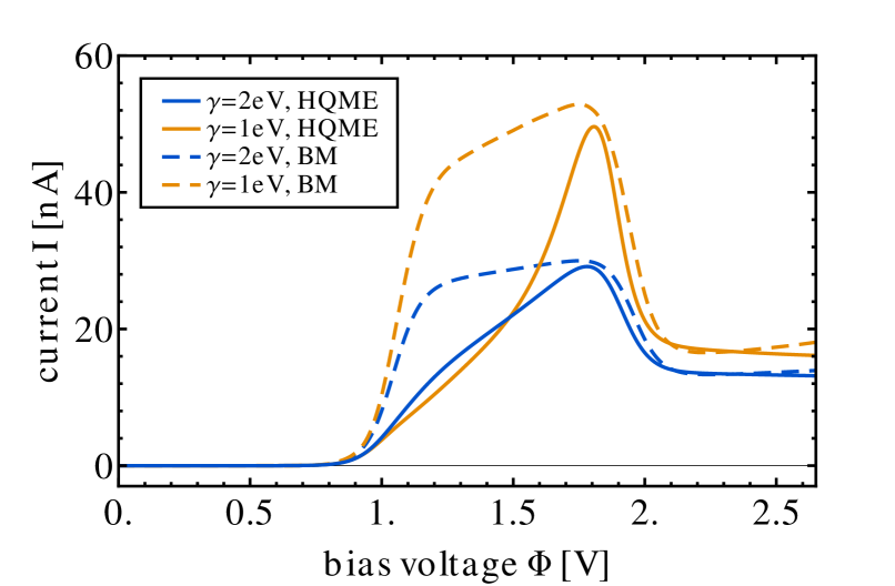
(b)

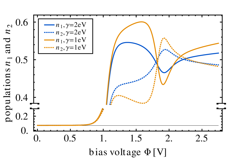
Figure 7: (Color online) Current-voltage and electronic population characteristics of junction DES for different band widths $\gamma$. The coupling parameter $\nu$ has been adjusted so that the maximal value of the level-width functions $\Gamma_{K,mn}$ is the same in all cases. The solid and dotted lines have been obtained by the HQME method. The dashed lines depict the corresponding current-voltage characteristics obtained by the BM scheme. Decoherence and lead induced inter-state coupling effects become stronger if the energy dependence of the level-width functions $\Gamma_{K,mn}$ is more pronounced.

III.1.3 Decoherence phenomena in the presence of finite electron-electron interaction strengths $U$

In the low and intermediate bias voltage regime $e\Phi<2\epsilon_{1/2}+U$ the finite $U$ case exhibits physics similar to that of the infinite-$U$ case (see Fig. 5). One difference is that the system with finite electron-electron interactions has a higher current while the difference in the electronic population is very similar. According to our analysis, the similarity in level occupation can be attributed to the off-diagonal elements $\Delta_{K,12}$ which have only a weak $U$ dependence. The associated current suppression, however, which arises from a modification of the effective level renormalization Wunsch et al. (2005) due to the effect of the $\Delta_{K,12}$, exhibits a non-negligible $U$-dependence. To corroborate this statement, the solid orange lines in Fig. 7 show the transport characteristic of junction DES calculated with a reduced band width $\gamma$, that is, effectively, with enhanced off-diagonal elements $\Delta_{K,12}(\epsilon)$. The current level of this junction is indeed reduced for bias voltages $e\Phi<2\epsilon_{1/2}+U$ while the difference in the electronic populations $n_{1}$ and $n_{2}$ is increased.

At higher bias voltages, $2\epsilon_{1/2}+U<e\Phi<2(\epsilon_{1/2}+U)$, the intermediate $U$ case exhibits a qualitatively different behavior from either the $U\rightarrow 0$ or $U\rightarrow\infty$ limits. The current of junction DES passes through a maximum value substantially larger than found in either of the limits and then decreases, exhibiting a regime of negative differential resistance. The maximum value is seen to be close to the one found in the BM scheme (cf. Fig. 5a or Fig. 7a). Moreover, in the voltage regime of the current peak and negative differential resistance, an inversion of the electronic population occurs (see Fig. 5b). These effects are related to the energy dependence of $\Gamma_{K,mn}(\epsilon)$ and arise when doubly occupied states enter the bias window. As we have already seen in the limit $U\rightarrow\infty$, state $1$ is populated more strongly than state $2$ for $\Phi<2\epsilon_{1/2}+U$. Thus, at higher bias voltages, adding another electron into state $2$ is more favorable than into state $1$. Due to electron-electron interactions, these addition processes occur at higher energies $\epsilon_{1/2}+U$ and, therefore, also with a higher probability because of the energy dependence of the level-width functions: $\Gamma_{\text{L},mn}(\epsilon_{1/2}+U)>\Gamma_{\text{L},mn}(\epsilon_{1/2})$ for $e\Phi\approx 2(\epsilon_{1/2}+U)$. When the population of the two levels is approximately the same, the effect of the off-diagonal elements $\Delta_{12}$ on the population dynamics is canceled. The associated current suppression also vanishes leaving the decoherence due to electron-electron interactions as the dominant effect. The real part of the coherence $\sigma_{10,01}$ and the current level thus reach a local minimum and a maximum, respectively. Once the bias voltage exceeds $2(\epsilon_{1/2}+U)$, resonant transport through one of the levels occurs irrespective of the population of the other level. Consequently, decoherence due to the reduction of the Hilbert space is no longer effective and the current level drops rapidly to the one of the non-interacting case. Also, the population of the two levels start to follow again the same rules as in the non-interacting limit.

The above analysis suggests that the maximal enhancement of the current due to decoherence by electron-electron interactions is not controlled by the value of the electron-electron interaction strength $U$. It rather enters via the asymmetry in the transfer rates $\Gamma_{\text{L},mn}(\epsilon_{1/2})$ and $\Gamma_{\text{R},mn}(\epsilon_{1/2})$ that increases with the applied bias voltage $\Phi$. This is confirmed by the current-voltage characteristics shown in Fig. 8 for different electron-electron interaction strengths $U$. As can be seen, the height of the current peaks for different values of $U$ follow the dashed gray line, which depicts the current-voltage characteristic obtained from the BM scheme in the limit $U\rightarrow\infty$. Thereby, the similarity to the BM $U\rightarrow\infty$ case is only present if the electron-electron interaction strength of the system is significantly larger than the broadening of the steps in the corresponding current-voltage characteristic. If the broadening exceeds the electron-electron interaction strength $U$, which, in our case, is given by the thermal broadening $k_{\text{B}}T\approx 25$ meV, the decoherence effect becomes quenched. The same would be true if the broadening due to the coupling to the electrodes is dominant or comparable to the thermal broadening, $\Gamma\gtrsim k_{\text{B}}T$, as can be inferred from the results of Wunsch et al. Wunsch et al. (2005). This also means that our findings remain valid at higher temperatures, as long as $U\gg k_{\text{B}}T$.

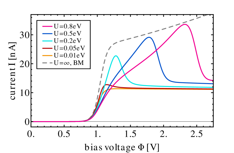
Figure 8: (Color online) Current-voltage characteristics of junction DES for different electron-electron interaction strengths, ranging from $U=0.8$ eV$\gg k_{\text{B}}T\approx 25$ meV to $U=0.01$ eV$\ll k_{\text{B}}T$. Decoherence due to electron-electron interactions is independent of the interaction strength $U$, as long as it exceeds the broadening induced by the coupling to the electrodes and temperature.

III.1.4 Asymmetric coupling to the electrodes

So far, we considered only scenarios in which the absolute values of the coupling parameters $|\nu_{K,m}|$ are the same. In an experimental realization of junction DES the system S may be coupled more strongly to one of the electrodes than to the other. The current-voltage characteristic of such a junction is shown as the solid red line in Fig. 9a. In comparison to junction DES (solid blue line), it is described by the same parameters except for a weaker coupling to the right electrode $\nu_{\text{R},1/2}=\nu/3$. The corresponding population of states 1 and 2 are depicted by the solid and dotted red lines in Fig. 9b. As can be seen, an asymmetric coupling to the electrodes introduces a number of quantitative differences, including a particle-hole asymmetry and changes to the heights and widths of the current peaks, but the qualitative behavior is the same as in the symmetric case. It is interesting to note that similar current-voltage characteristics have been observed by Osorio et al. Osorio et al. (2010) but only if the corresponding molecular junctions are in a low-current state.

(a)

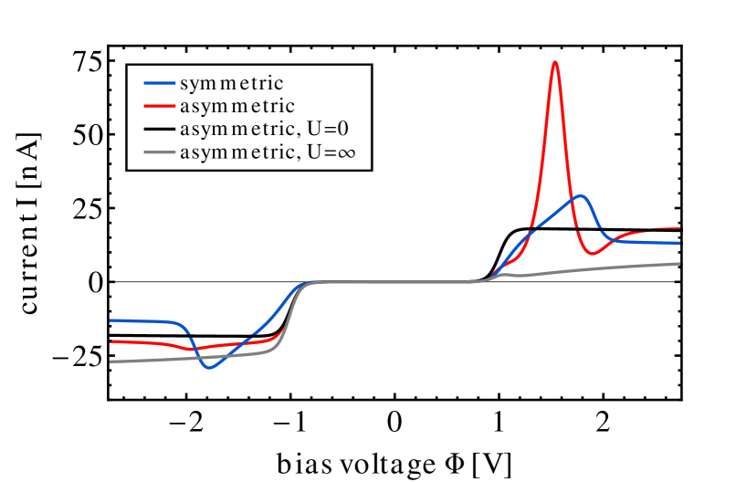
(b)

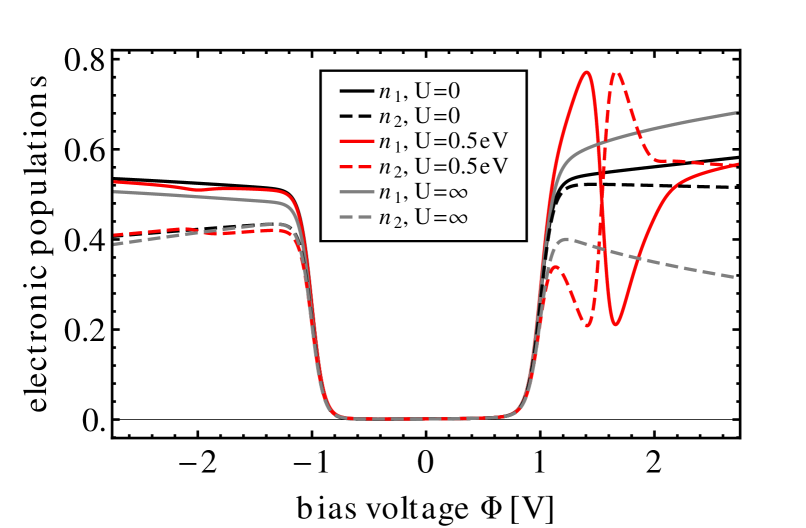
Figure 9: (Color online) Panel (a): Current-voltage characteristics of the symmetrically coupled junction DES (solid blue line) and a very similar junction, where the coupling to the right lead is reduced by $1/3$ (red line). For comparison, the black and gray line show the current-voltage characteristics of the asymmetrically coupled system in the limit $U=0$ and $U=\infty$, respectively. Panel (b): Electronic population characteristics of the asymmetrically coupled system. Asymmetric coupling to the leads enhances the effect of population inversion and decoherence due to electron-electron interaction for one bias polarity, while for the other polarity both effects are attenuated.

The asymmetry with respect to bias voltage may be understood as follows. For positive bias voltages, where transport occurs from L$\rightarrow$S$\rightarrow$R, the two levels are populated on faster time scales than they become depopulated. Thus, the population of level $1$ is significantly larger at the onset of the resonant transport regime at $e\Phi=2\epsilon_{1/2}$. At this value of $\Phi$ the repulsive electron-electron interactions mean that the population of state $2$ is more strongly suppressed (cf. Fig. 9b). The same arguments apply at higher bias voltages, $2\epsilon_{1/2}+U<e\Phi<2(\epsilon_{1/2}+U)$, where the population of the two levels become inverted once the doubly occupied states enter the bias window (cf. the discussion given in Sec. III.1.3). Thus, the current suppression due to the blocking of transport channels is more pronounced than for the symmetrically coupled junction such that, at $e\Phi\approx 2\epsilon_{1/2}$ and $e\Phi\approx 2(\epsilon_{1/2}+U)$, the current level drops to half of the level in the non-interacting case. This results also in a narrowing and a shift of the current peak to lower bias voltages. Compared to the symmetrically coupled scenario, the height of this peak is substantially increased, indicating that decoherence due to the reduced Hilbert space for the tunneling electrons is more pronounced. This is related to the reduced values of $\Gamma_{K,mn}$ in the same way as the increase of the current level in the limit $U\rightarrow\infty$ (cf. Sec. III.1.2). Studying the ratio of the peak height versus the current level of the non-interacting case (which is equivalent to the current at $\Phi=3$ V), one finds that this enhancement of the current peak is most pronounced for an asymmetry ratio $|\nu_{\text{R},1/2}|/|\nu_{\text{L},1/2}|\approx 0.4$ (cf. Fig. 10).

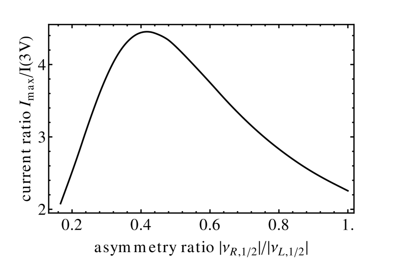
Figure 10: (Color online) Ratio between the maximal current and the current level at $\Phi=3$ V for junction DES as a function of the asymmetry ratio $|\nu_{\text{R},1/2}|/|\nu_{\text{L},1/2}|$. The peak in this curve reveals that decoherence due to electron-electron interactions is most effective for intermediate asymmetries in the system-electrode coupling

At yet larger bias voltages, $e\Phi>2(\epsilon_{1/2}+U)$, destructive interference effects are fully developed and dominate the suppression of transport processes. The same holds true at negative bias polarities, where the time scales for populating and depopulating the two states are reversed such that electron-electron interactions and the corresponding decoherence mechanisms are, a priori, less pronounced. It is also interesting to note that, at these bias voltages, the current level of the asymmetrically coupled junction is slightly larger than for the symmetrically coupled one, despite the reduced coupling to the right lead. The physical origin of this behavior is that, again, destructive interference effects are less effective if the system is less strongly coupled to the electrodes Härtle et al. (2013a).

III.1.5 Gate-voltage dependence

Besides a source and a drain electrode, one often uses a third, so-called gate electrode to study the transport properties of a nanoelectronic device Tans et al. (1997); Ihn et al. (2007); Ballmann and Weber (2012). Such an electrode is capacitively coupled to the junction and acts to shift the level positions $\epsilon_{m}$ with respect to the Fermi levels of the leads. Dependence on gate voltage can help to reveal the nature of conduction processes. Sequential tunneling may be distinguished from higher-order processes such as cotunneling or spin-flip (due to Kondo physics) Tews (2004); Begemann et al. (2010) by its much stronger gate-voltage dependence. In the following, we study the gate voltage dependence of the transport properties of junction DES by assuming that the gate voltage shifts the level energies as $\epsilon_{m}\rightarrow\epsilon_{m}+e\Phi_{\text{gate}}$.

Fig. 11a presents a conductance map for junction DES in the plane of gate and source-drain voltage with negative conductance depicted in blue, zero in white and positive conductance in red. The conductance map is symmetric with respect to both the bias voltage $\Phi$ and the gate-voltage $\Phi_{\text{gate}}$. The two symmetry axes cross at the charge-symmetric point $(e\Phi,e\Phi_{\text{gate}})=(0,-2\epsilon_{1/2}-U)\approx(0,-0.75$ eV$)$. We therefore restrict the discussion to the upper right quarter of this map in the following. For gate-voltages $0>e\Phi_{\text{gate}}>-2\epsilon_{1/2}\approx-0.5$ eV, the onset of the resonant transport regime at $e\Phi=2(\epsilon_{1/2}+\Phi_{\text{gate}})$ as well as the NDR feature appearing at bias voltages slightly higher than the resonant tunneling onset decrease linearly with the applied gate voltage. For yet smaller gate voltages, $-2\epsilon_{1/2}>e\Phi_{\text{gate}}>-2\epsilon_{1/2}-U$ where $\epsilon_{1/2}+e\Phi_{\text{gate}}<0$, this trend is reversed. In addition, a more complex structure emerges, as the current drops in two steps at $e\Phi\gtrsim-2(\epsilon_{1/2}+e\Phi_{\text{gate}})$ and $e\Phi\lesssim 2(\epsilon_{1/2}+U+\Phi_{\text{gate}})$. The current maximum and the corresponding NDR vanish as the system is driven to the charge-symmetric point (at $e\Phi_{\text{gate}}=-2\epsilon_{1/2}-U$).

(a)	(b)

Figure 11: (Color online) Panel (a) and (b) depict the differential conductance $\text{d}I/\text{d}\Phi$ and the difference in the electronic populations $n_{1}-n_{2}$ of junction DES as a function of both bias and gate voltage. Comparison shows that the occurrence of negative differential resistance (blue areas) is correlated with population inversion (turquoise areas) in the resonant transport regime.

The nature of the additional drop in the current can be revealed by inspection of the conductance map obtained from the BM master equation scheme shown in Fig. 12. In the range of gate voltages from $-2\epsilon_{1/2}$ to $-2\epsilon_{1/2}-U$, the onset of the resonant transport regime at $e\Phi=-2(\epsilon_{1/2}+e\Phi_{\text{gate}})$ does not appear as a step but as a peak in the respective current-voltage characteristic. This is reflected by high positive conductance values for $e\Phi\lesssim-2(\epsilon_{1/2}+e\Phi_{\text{gate}})$ followed by negative values for $e\Phi\gtrsim-2(\epsilon_{1/2}+e\Phi_{\text{gate}})$. The consecutive drop of the current at $e\Phi\sim 2(\epsilon_{1/2}+U+e\Phi_{\text{gate}})$ is almost the same as for higher gate voltages, $0>e\Phi_{\text{gate}}>-2\epsilon_{1/2}$. The appearance of the current peaks is related to the fact that, for $e\Phi\lesssim-2(\epsilon_{1/2}+e\Phi_{\text{gate}})$, transport processes occur via a thermally assisted tunneling process from the junction into the right lead, followed by another tunneling process from the left lead onto the junction. While the former exhibits partial Pauli-blocking, the latter does not and, therefore, involves electrons with a wider range of energies. As a result, destructive interference effects cannot fully develop. This results in a more pronounced increase of the current level than for thermally assisted transport through the unoccupied (or doubly occupied) system. For larger bias voltages, $e\Phi\gtrsim-2(\epsilon_{1/2}+e\Phi_{\text{gate}})$, the Pauli-blocking of the tunneling process into the right electrode is no longer active and destructive interference effects start to suppress the current flow through the junction, reducing the current level again.

Figure 12: (Color online) Conductance map similar to the one shown in Fig. 11a but obtained using the BM master equation scheme (cf. Sec. II.3). Comparison of Figs. 11a and 12 reveals the strong renormalization effects that are induced by lead induced inter-state coupling encoded in the off-diagonal elements $\Delta_{12}$.

Considering again Fig. 11a, where, in contrast to Fig. 12, the real part of the self-energy matrix $\mathbf{\Sigma}$ is taken into account, one observes a strong renormalization of the above described temperature-induced decoherence effects, in particular of the current peaks at $e\Phi\gtrsim-2(\epsilon_{1/2}+e\Phi_{\text{gate}})$. On one hand, they become quenched the closer the system is driven to the charge-symmetric point (i.e. for gate voltages $\Phi_{\text{gate}}\approx-(\epsilon_{1/2}+U/2)=-0.75$ V). Thereby, it should be noted that the renormalization of these peaks leads to signatures around zero bias that appear to be similar (but must not be mistaken) as signatures due to pseudo-Kondo Boese et al. (2001); Lee and Kim (2007) or Kondo-like correlations Cronenwett et al. (1998); Goldhaber-Gordon et al. (1998); Liang et al. (2002). On the other hand, these peaks appear much broader. While this broadening exceeds the thermal broadening ($\approx 25$ meV) or the broadening due to the coupling to the electrodes ($\approx 2$ meV) by more than an order of magnitude, it is most pronounced around the charge-symmetric line, i.e. for $\Phi_{\text{gate}}\approx-0.75$ V, where it amounts to $\sim 0.5$ eV. The other (electronic) signatures of the conductance map exhibit similar broadening. Note that such a pronounced broadening of electronic signatures has recently been experimentally observed in the transport characteristics of a number of single-molecule junctions Secker et al. (2011), where, however, it has been attributed to electronic-vibrational coupling Ness and Fisher (2005); Secker et al. (2011).

Fig. 11b shows the difference in the electronic populations $n_{1}$ and $n_{2}$. Comparison to Fig. 11a reveals that the appearance of negative differential resistance is closely linked to population inversion (turquoise areas) in the resonant transport regime. In the non-resonant transport regime and gate voltages $-2\epsilon_{1/2}>e\Phi_{\text{gate}}>-2\epsilon_{1/2}-U$, the population of the higher lying level is also more pronounced, although the current is monotonously increasing. As this behavior is not observed using the Born-Markov scheme, we also attribute it to the inter-state coupling effects induced by the off-diagonal elements $\Delta_{12}$. Note that the corresponding relaxation time scale is three orders of magnitude larger in this regime (ns instead of ps). We therefore computed the detailed data shown in Figs. 11a and 11b by truncating the hierarchy of equations of motion (II.2) at the first tier. We checked that the results that have been discussed in this section are not affected by this choice of the truncation scheme.

III.1.6 Comparison to blocking state scenarios

The mechanism for negative differential resistance that we investigate in this article is based on decoherence due to electron-electron interactions. Another well-known mechanism for NDR due to electron-electron interactions involves electronic states that are weakly coupled to the electrodes. This includes blocking states Hettler et al. (2002, 2003); Muralidharan and Datta (2007); Härtle and Thoss (2011b); Leijnse et al. (2011) which are weakly coupled to only one of the electrodes as well as centrally localized states Härtle and Thoss (2011b) which are weakly coupled to both electrodes (or, similarly, spin-blockade in systems that are coupled to ferromagnetic leads Braun et al. (2004)). In these systems, NDR occurs when the weakly coupled state enters the bias window, leading to similar features in the current-voltage characteristic than the decoherence mechanism outlined before. Inspection of the respective conductance maps, however, reveals important qualitative differences.

Fig. 13a and 13b show conductance maps of junctions with a centrally localized (model CENTRAL) and a blocking state, respectively (model BLOCK). A detailed list of the corresponding model parameters is found in Tab. 1. The most important difference between NDR due to decoherence and NDR due to weakly coupled states is the symmetry with respect to the applied gate voltage. While decoherence leads to symmetric NDR features, weakly coupled states result in NDR that is non-symmetric with respect to the gate voltage $\Phi_{\text{gate}}$. Moreover, areas where NDR occurs terminate in different ways at the central Coulomb diamond. While these areas almost touch each other when NDR is induced by decoherence, they terminate at the sides of the diamond when NDR is the result of weakly coupled states. Note that an asymmetric coupling to one of the electrodes, for example a weaker coupling to the right electrode, attenuates the NDR features only in the upper left and the lower right corner (similar as in Fig. 13b), irrespective of the underlying mechanism (data not shown).

a)	b)

Figure 13: (Color online) Conductance maps of junctions with a centrally localized state (Panel (a)) and a blocking state (Panel (b)).

III.1.7 Influence of the type of conduction bands: Comparison to NCA

In this section we use the NCA (cf. Sec. II.4) to investigate the interplay between decoherence and correlation in junction DES. The NCA is an infinite order resummation of a selected subset of diagrams in a hybridization expansion. As will be seen, it reproduces some of the qualitative behavior that is found by the numerically exact HQME method, although it also misses other aspects and is quantitatively inaccurate. An advantage, however, is that it facilitates the study of non-Lorentzian density of states. As an example, we present here results obtained using semi-elliptical conduction bands

$$\Gamma_{K,mn}\left(\epsilon\right)=2\pi\frac{\nu_{K,m}\nu_{K,n}}{\gamma}\sqrt{1-\frac{\epsilon^{2}}{\gamma^{2}}},$$ (40)

For numerical convenience we slightly modified the functional dependence at the band edges, replacing the square root singularity by an exponential decay, so $\Gamma_{K,mn}(\epsilon)=Ae^{-\alpha\left|\epsilon-\mu_{K}\right|}$ when $|\epsilon-\mu_{K}|>\epsilon_{c}$, where $\Gamma_{K,mn}(\epsilon_{c})=0.5\Gamma_{K,mn}(\mu_{K})$ and the parameters $A$ and $\alpha$ are chosen such that $\Gamma_{K,mn}$ and its first derivative are continuous. The resulting level-width function(s) and the respective real parts of the self energy are depicted in Fig. 14.

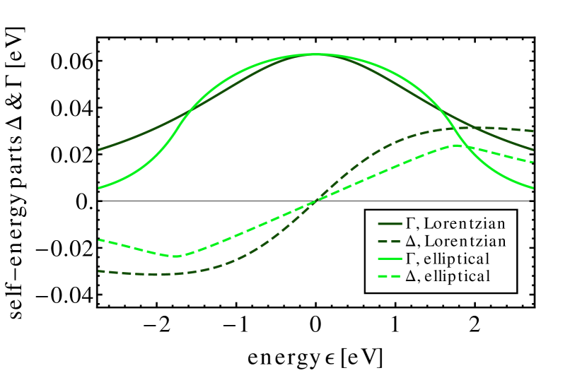
Figure 14: (Color online) Level-width functions and the corresponding real parts of the self energy as a function of energy $\epsilon$. The dark green lines refer to Lorentzian conduction bands (cf. Eq. 5), while the light green lines are associated with the (modified) semi-elliptical bands (cf. Eq. (40)).

The corresponding current-voltage and electronic population characteristics are represented by the turquoise lines in Fig. 15. For comparison, the dark red lines show results that have been computed using Lorentzian conduction bands (cf. Eq. (5)). The basic decoherence phenomena found for the Lorentzian density of states also occur for elliptical conduction bands, in particular the inter-state coupling effects encoded in the off-diagonal elements $\Delta_{12}$, that is an enhanced broadening of electronic signatures and population inversion. While the NCA captures these effects qualitatively, it is also evident that it fails on both a quantitative and a qualitative level. According to our previous analysis, for example, the differences in the electronic population should be less pronounced because the real parts of the corresponding self-energy matrix are smaller (cf. Fig. 14). This picture can be confirmed very easily in the non-interacting case, using, for example, the Green’s function analysis outlined in Sec. III.1.1. However, it is reproduced by the NCA results only in parts. In particular, the difference of the electronic populations at the onset of the resonant transport regime $e\Phi\approx 2\epsilon_{1/2}$ and for higher bias voltages $e\Phi>2(\epsilon_{1/2}+U)$ is not smaller but larger in the elliptical case. This already indicates that the partial resummation of the NCA diagrams is not sufficient to describe this transport problem.

(a)

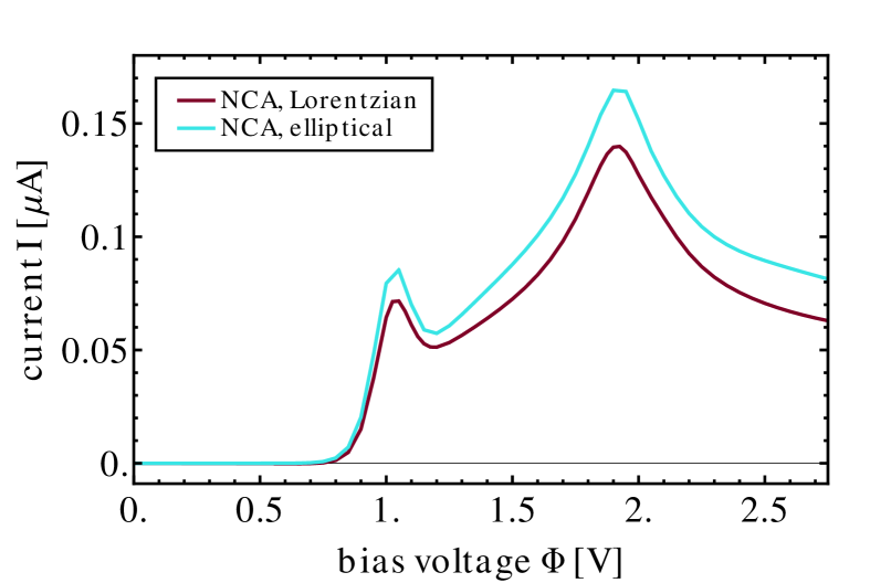
(b)

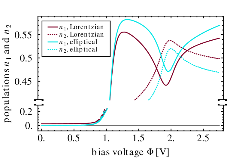
Figure 15: (Color online) Current-voltage and electronic population characteristics of junction DES. The turquoise and red curves depict results that are obtained with the NCA scheme for elliptical and Lorentzian conduction bands, respectively.

A direct comparison of the NCA results with the ones obtained by the BM and the HQME approach reveals further inaccuracies. To this end, we show the current-voltage characteristics of junction DES in Fig. 16 that have been obtained by the three methods using Lorentzian conduction bands. Again, while the NCA captures some aspects of the problem, like the decoherence-induced negative differential resistance, it also shows qualitative differences. This includes an additional current peak at $e\Phi\approx 2\epsilon_{1/2}$ but, more importantly, also much higher current levels. Thus, NCA underestimates the effect of destructive interference effects in this system. Future work may show if these deficiencies can be overcome using the one-crossing (or higher) approximation in order to obtain qualitatively or even quantitatively correct results Grewe et al. (2008). Note that another nonequilibrium example where NCA fails in the presence of non-degenerate levels is given in Ref. Cohen et al. (2013b).

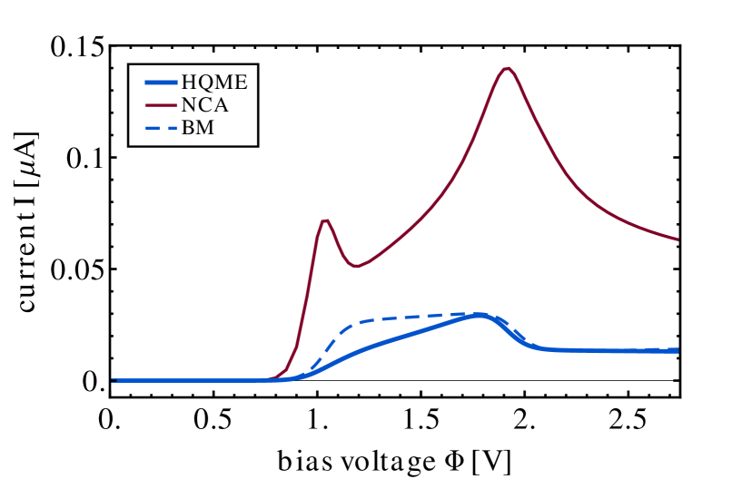
Figure 16: (Color online) Current-voltage characteristics of junction DES obtained by three different methods: the HQME method (blue line), the NCA (dark red line) and the Born-Markov scheme (dashed blue line).

III.1.8 Higher order effects

At this point, some remarks about higher order effects and numerics are in order. Fig. 17 presents current-voltage characteristics for junction DES, employing different truncation levels of the hierarchy (II.2). Thereby, we focus on the non-resonant transport regime, $e\Phi<2\epsilon_{1/2}$, where resonant processes are energetically not accessible or Pauli-blocked and, consequently, higher order effects are dominant. This requires a theoretical description beyond the leading order in $\Gamma$ Pedersen et al. (2007); Leijnse and Wegewijs (2008); Esposito and Galperin (2010). In the HQME methodolody, the depth of such an expansion can be controlled by the threshold value $A_{\text{th}}$, where lower values correspond to a higher quality of the result. The details of the truncation scheme are outlined in App. A. Tab. 2 summarizes the number of auxiliary operators $\sigma^{(\alpha)}_{j_{1}..j_{\alpha}}$ that are included in these calculations at every tier. The number of auxiliary operators in the $\alpha$th tier can be estimated as $\gamma^{\alpha-1}/((k_{\text{B}}T)^{\alpha-1}A_{\text{th}}\alpha!)$ (cf. App. A). In the resonant transport regime, we observe only marginal variations in the transport characteristics of junction DES as the truncation level is changed, because the first tier, including the effect of resonant processes, is always fully accounted for by our scheme.

		$10^{0}$			$10^{-1}$			$10^{-2}$			$10^{-3}$			$10^{-4}$			$10^{-5}$
1		202			202			202			202			202			202
2		0			12			97			423			1530			3486
3		0			0			0			17			311			1965
4		0			0			0			0			0			7

Table 2: Number of auxiliary operators in each tier $\alpha$ for different threshold values $A_{\text{th}}$. Thereby, the first hundred Matsubara frequencies $\omega^{s}_{K,1..100}$ are included in order to obtain converged results.

		$10^{0}$			$10^{-1}$			$10^{-2}$			$10^{-3}$			$10^{-4}$			$10^{-5}$
1		62			62			62			62			62			62
2		0			10			85			392			1381			2896
3		0			0			0			12			235			1442
4		0			0			0			0			0			3

Table 3: Number of auxiliary operators in each tier $\alpha$ for different threshold values $A_{\text{th}}$ if, instead of the Matsubara decomposition scheme, the Pade approximation Ozaki (2007); Hu et al. (2010, 2011) is employed. Thereby, we included the first thirty poles of this decomposition scheme in order to obtain converged results.

The results are converged to a satisfactory level if $A_{\text{th}}\lesssim 10^{-5}$. They are the same as if all auxiliary operators of the zeroth, first and second tier are included while all other auxiliary operators are discarded (data not shown). Unphysical negative currents are obtained for higher threshold values $A_{\text{th}}\gtrsim 10^{-2}$, which corresponds to the same level of accuracy as the BM master equation scheme including, however, the real part of the self-energy due to the coupling to the electrodes. This shows both the importance of second order effects, which are only well represented for $A_{\text{th}}\lesssim 10^{-4}$, and the stability of our results with respect to higher order effects. Decoherence due to electron-electron interactions is less pronounced in the non-resonant transport regime, because the population of the two levels is negligible, $n_{1/2}\approx 0$.

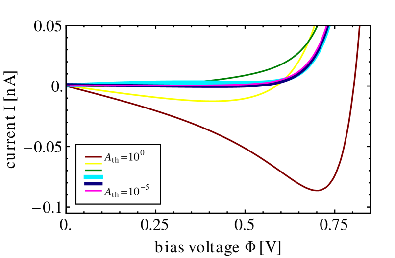
Figure 17: (Color online) Current-voltage characteristics of junction DES for different depths of the hierarchy of auxiliary operators (controlled by the threshold value $A_{\text{th}}$). At the lowest level, only resonant processes are included, while, upon increasing the depth of the hierarchy, higher order processes enter successively. Unphysical results are obtained in the non-resonant transport regime, i.e. for $e\Phi<2\epsilon_{1/2}\approx 1$ V, if the depth of the hierarchy is too low.

For comparison we also show the number of auxiliary operators in Tab. 3 that would have been required using the alternative Pade approximation scheme Ozaki (2007); Hu et al. (2010, 2011). The results are almost identical to the ones shown in Fig. 17 (data not shown). Although the Pade approximation is, in general, more efficient, the increase is limited. In the present case, the number of auxiliary operators is reduced by a factor of only $1.2$, while a factor of about two can be obtained for lower temperatures. This is because the Pade and the Matsubara decomposition scheme share half of the frequencies (18) and the amplitudes (21). Moreover, the similarity of results and the small gain in numerical efficiency points out the quality of our truncation scheme (see App. A).

III.2 Transport properties of junction CON

To complete our discussion, we discuss the transport properties of the complementary model system CON. The corresponding current-voltage and population characteristics are shown in Fig. 18 (blue lines). For comparison, we also show the transport characteristics of this junction if electron-electron interactions are neglected (black lines) and for the limit $U\rightarrow\infty$ (gray lines). All three scenarios exhibit NDR in the resonant transport regime. In contrast to junction DES, the NDR is not very pronounced and not related to decoherence effects but rather a direct consequence of the finite band width $\gamma$ which results in a reduced overlap of the conduction bands at $\epsilon\approx\epsilon_{1/2}$ and $\epsilon\approx\epsilon_{1/2}+U$ and, thus, in reduced current levels if the bias voltage is increased. Note that this mechanism for NDR is counterbalanced in junction DES, because destructive interference effects become simultaneously less pronounced.

(a)

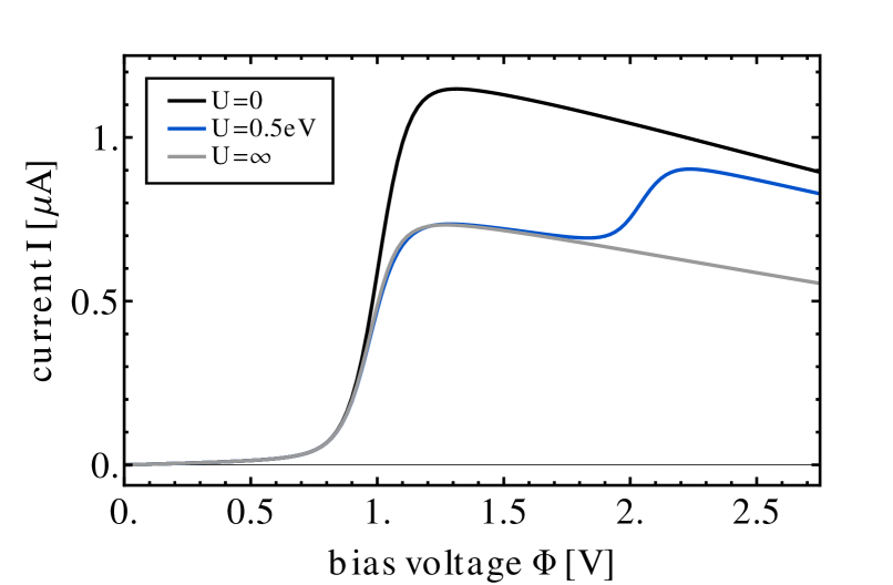
(b)

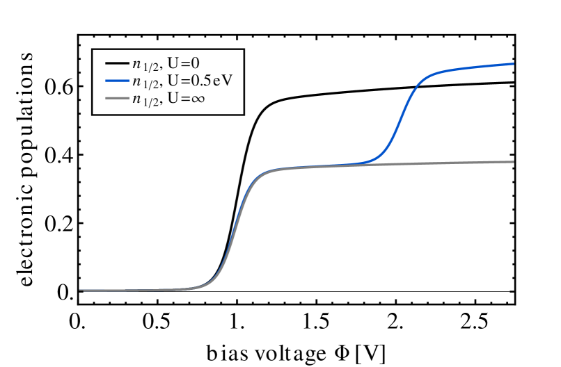
Figure 18: (Color online) Current-voltage and electronic population characteristics of junction CON. Interference effects and decoherence due to electron-electron interactions is less pronounced in this system.

Fig. 18a also shows that the current level of junction CON is suppressed for bias voltages $2\epsilon_{1/2}<e\Phi<2(\epsilon_{1/2}+U)$. In this regime of bias voltages, the junction can be populated via two channels but depopulated only via a single channel. The corresponding current can thus be estimated as $2\Gamma^{2}/(2\Gamma+\Gamma)$, corresponding to a reduction of the current by a factor of $2/3$. This blocking of transport channels is also reflected in the population of the electronic levels $1$ and $2$, where the aforementioned asymmetry in the population and depopulation dynamics of the junction results in an average population of $\simeq 1/3$. At higher bias voltages, both levels are populated simultaneously and the average population increases. It exceeds $0.5$ due to the finite band width $\gamma$.

In comparison to junction DES, interference and lead induced inter-state coupling effects play no role for the transport properties of junction CON. The population of the two eigenstates is almost identical, $n_{1}\approx n_{2}$, and the coherence $\sigma_{10,01}$ takes very low values ($|\sigma_{10,01}|\lesssim 10^{-3}$, data not shown). This seems counterintuitive at first, since the quasidegeneracy of the eigenstates and the symmetry of the coupling strengths $\nu_{K,m}$ implies strong constructive interference effects. Such effects indeed double the current level of the system in the non-resonant transport regime Härtle et al. (2013a). At higher bias voltages, however, an antiresonance at $\epsilon=(\epsilon_{1}+\epsilon_{2})/2$ cancels the effect of constructive interference effects (cf. Ref. Härtle et al., 2013a for a more detailed discussion). This behavior can also be understood in terms of the weak coupling between the dots (cf. Fig. 1), which effectively factorizes the corresponding population dynamics. As a result, electron-electron interactions have only an electrostatic influence in this system. A similar behavior is obtained if $|\epsilon_{2}-\epsilon_{1}|>\Gamma$ (even for junction DES).

According to this analysis, junctions DES and CON can be viewed as two extreme cases, where decoherence due to electron-electron interactions is fully developed and where it plays no role, respectively. It is thus interesting to note that the BM scheme is also capable of describing resonant transport through junction CON both qualitatively and quantitatively (except for the broadening due to the coupling to the electrodes, data not shown).

IV Conclusion

We have investigated the electrical transport properties of an interacting double quantum dot system with quasidegenerate electronic states, focusing on decoherence phenomena due to electron-electron interactions and employing a modified version of the numerically exact HQME approach of Jin et al. Jin et al. (2008). The HQME approach allowed us to validate our results with respect to higher-order ($\geq 2$) effects in a systematic, numerically exact way. This is crucial in the present context, as the most important effects are associated with sequential tunneling Pedersen et al. (2007) while, concurrently, a strict second order expansion yields unphysical results in some parameter regimes. In addition, a comparison of the HQME and the BM scheme elucidated strong inter-state coupling effects that originate in these systems from the energy dependence of the tunneling efficiency between the dots and the electrodes. We find that interaction-induced decoherence gives rise to pronounced negative differential resistance Wunsch et al. (2005); Pedersen et al. (2007); Trocha et al. (2009), an enhanced broadening of the corresponding electronic signatures and an inversion of the electronic population of the junction (cf. Fig. 7). We found that these phenomena can be even more pronounced for intermediate asymmetries in the coupling to the electrodes. An important experimental signature which distinguishes decoherence-induced NDR from other mechanisms, for example a centrally localized or a blocking state, is the symmetry with respect to a gate voltage around the charge symmetric point (compare Figs. 11a and 13).

The decoherence mechanism that underlies these effects is based on the blocking of (doubly occupied) states. The principal effects are thus only weakly dependent on the electron-electron interaction strength and enter only via the relative position of resonances as well as the energy dependence of the tunneling efficiency between the dots and the electrodes. The enhanced broadening of electronic signatures in the transport characteristics and the inversion of the electronic population can be solely attributed to the effect of the latter and the associated inter-state coupling while the shape of the associated current peaks or the appearance of negative differential resistance is also strongly modified. As a consequence, the corresponding conductance map shows resonance lines that can be disconnected, bent and even smeared out (compare Figs. 11a and 12). These results have been further corroborated by studying different functional forms of the tunneling efficiency between the dots and the electrodes using NCA. While the BM and the NCA method capture but also miss some of the qualitative aspects, they fail to describe the transport characteristics of these systems on a quantitative level. Note that, according to the results of Pedersen et al. Pedersen et al. (2007), one can expect that the decoherence effects described in this work are even more pronounced for the spinful case.

Appendix A Numerical solution of the hierarchical equations of motion

The hierarchical equations of motion (II.2) are numerically integrated using the Euler method. Thereby, the initial conditions are set to the state where the system is initially unpopulated. Other initial conditions, associated with the singly occupied and doubly occupied system, have also been considered. The steady state properties studied in this article did not show any dependence on the choice of the initial states. In this context it should be noted that all auxiliary operators are identical to zero at $t=0$. This can be inferred from the definitions (II.2) and (26) and corresponds to the choice that the system S and the electrodes L and R are initially uncorrelated.

The numerical effort in the evaluation of the hierarchical of equations of motion (II.2) can be reduced, using that

$$\left(\sigma^{(\alpha)}_{j_{1}..j_{\alpha}}(t)\right)^{\dagger} = (-1)^{\sum_{\beta=1..\alpha}\beta}\sigma^{(\alpha)}_{\overline{j}_{1}..\overline{j}_{\alpha}}(t),$$ (41)

where $\overline{j}_{1}=(K_{\beta},m_{\beta},\overline{s}_{\beta},p_{\beta})$, and

$$B_{j_{1}}B_{j_{2}} = -B_{j_{2}}B_{j_{1}}.$$ (42)

The latter identity implies that the auxiliary operators $\sigma^{(\alpha)}_{j_{1}..j_{\alpha}}(t)$ are identical to zero if two of the superindices $j_{1}$ – $j_{\alpha}$ coincide Jin et al. (2008). It should be noted at this point that there is, in general, an infinite number of superindices $j_{\beta}$ and, accordingly, of auxiliary operators such that the hierarchy of equations of motion (II.2) does in general not terminate automatically. Only in specific limits, in particular the non-interacting limit ($U=0$) or for $U\rightarrow\infty$, the hierarchy of equations of motion (II.2) truncates automatically at the second tier Jin et al. (2008, 2010). Respecting the relations (41) and (42), the number of auxiliary operators is given by $2^{N-1}$, where $N$ denotes the number of different superindices $j_{\beta}$.

The above result for the number of auxiliary operators only applies if all tiers of the hierarchy (II.2) are taken into account. In practice, however, it is truncated at a finite tier $\alpha$. This reduces the number of auxiliary operators considerably to $\sum_{\beta=1..\alpha}\frac{N!}{2\beta!(N-\beta)!}\sim N^{\alpha}/\alpha!$. The number of auxiliary operators can be reduced even further, because the frequencies $\omega_{K,p}^{s}$ and the amplitudes $\eta^{s}_{K,p}$ typically vary by orders of magnitude. The amplitudes $\eta^{s}_{K,p}$ enter the definition of the auxiliary operators as $\prod_{\beta=1..\alpha}\eta^{s_{\beta}}_{K_{\beta},p_{\beta}}$ (cf. Eq. (26)), while the real parts of the frequencies $\text{Re}[\omega^{\pm}_{K,p}]$ determine the time scales, where the dynamics of the system influences these quantities. The relative importance of the auxiliary operators $\sigma^{(\alpha)}_{j_{1}..j_{\alpha}}(t)$ can thus be assessed by the dimensionless amplitude $\prod_{\beta=1..\alpha}|\eta^{s_{\beta}}_{K_{\beta},p_{\beta}}|/\text{Re}[\omega^{s_{\beta}}_{K_{\beta},p_{\beta}}]$. Furthermore, the importance of the respective tier level $\alpha$ can be estimated by the prefactors $\nu_{K_{\alpha},m_{\alpha}}\nu_{K_{\alpha},n_{\alpha}}/\gamma$ and the sum of the frequencies $\sum_{\beta=1..\alpha}\omega_{K_{\beta},p_{\beta}}^{s_{\beta}}$, which link auxiliary operators of different tiers in Eqs. (II.2), in particular when the system is close to a stationary state. Therefore, in practical calculations, we neglect all auxiliary operators in the second and higher tier that have a dimensionless amplitude $\left|\gamma^{1-\alpha}\left(\prod_{\beta=1..\alpha-1}\nu_{K_{\beta},n_{\beta}}^{2}/\sum_{\beta^{\prime}=1..\beta}\text{Re}[\omega^{s_{\beta^{\prime}}}_{K_{\beta^{\prime}},p_{\beta^{\prime}}}]\right)\cdot\left(\prod_{\beta=1..\alpha}\eta^{s_{\beta}}_{K_{\beta},p_{\beta}}/\text{Re}[\omega^{s_{\beta}}_{K_{\beta},p_{\beta}}]\right)\right|$ that is smaller than a threshold value $A_{\text{th}}$. This value is reduced and, concurrently, the number of auxiliary operators in the first tier is increased until converged results are obtained. Note that, due to this choice of the amplitudes, it is not relevant whether the factor $\pi$, which appears in Eqs. (21), is included in the amplitudes $\eta_{K,p}^{s}$ or in the prefactors $\nu_{K_{\alpha},m_{\alpha}}\nu_{K_{\alpha},n_{\alpha}}/\gamma$.

Using this truncation scheme, the numerical effort can thus be reduced to a feasible level, as is further discussed in Sec. III.1.8. The numerical effort scales as $\sim N^{\alpha-1}/\alpha!$ considering that the amplitude condition cuts out a hypersurface of the total index space. For the specific parametrization scheme employed in Eq. (15) this statement can be formulated more explicitly. As

$$|\eta_{K,p}^{s}|/\text{Re}[\omega_{K,p}^{s}]\sim\frac{1}{2p-1}\frac{1}{(2p-1)^{2}-(\frac{\gamma}{k_{\text{B}}T})^{2}}$$ (43)

an upper bound for the width and the radius of the corresponding hypersurface may be estimated as $\sim 1/A_{\text{th}}$ and $\sim\gamma/(k_{\text{B}}T)$, respectively. Accordingly, the number of auxiliary quantities at each tier $\alpha$ scales as $\gamma^{\alpha-1}/((k_{\text{B}}T)^{\alpha-1}A_{\text{th}}\alpha!)$. Finally, it should be noted that the density and all auxiliary operators include $2^{N_{\text{el}}}$ matrix elements.

References

- Kastner (2000) M. A. Kastner, Ann. Phys. (Leipzig) 9, 885 (2000).
- Cuevas and Scheer (2010) J. C. Cuevas and E. Scheer, Molecular Electronics: An Introduction To Theory And Experiment (World Scientific, Singapore, 2010).
- Chang et al. (1974) L. L. Chang, L. Esaki, and R. Tsu, Appl. Phys. Lett. 24, 593 (1974).
- Davies et al. (1993) J. H. Davies, S. Hershfield, P. Hyldgaard, and J. W. Wilkins, Phys. Rev. B 47, 4603 (1993).
- Mizuta and Tanoue (1995) H. Mizuta and T. Tanoue, The Physics and Applications of Resonant Tunneling Diodes (Cambridge University Press, New York, 1995).
- Stafford et al. (2007) C. A. Stafford, D. M. Cardamone, and S. Mazumdar, Nanotechnology 18, 424014 (2007).
- Saha et al. (2010) K. K. Saha, B. K. Nikolic, V. Meunier, W. Lu, and J. Bernholc, Phys. Rev. Lett. 105, 236803 (2010).
- Ballmann et al. (2012) S. Ballmann, R. Härtle, P. B. Coto, M. Elbing, M. Mayor, M. R. Bryce, M. Thoss, and H. B. Weber, Phys. Rev. Lett. 109, 056801 (2012).
- Kießlich et al. (2007) G. Kießlich, E. Schöll, T. Brandes, F. Hohls, and R. J. Haug, Phys. Rev. Lett. 99, 206602 (2007).
- Brun et al. (2012) C. Brun, K. H. Müller, I. P. Hong, F. Patthey, C. Flindt, and W. D. Schneider, Phys. Rev. Lett. 108, 126802 (2012).
- Cronenwett et al. (1998) S. M. Cronenwett, T. H. Oosterkamp, and L. P. Kouwenhoven, Science 281, 540 (1998).
- Goldhaber-Gordon et al. (1998) D. Goldhaber-Gordon, H. Shtrikman, D. Mahalu, D. Abusch-Magder, U. Meirav, and M. A. Kastner, Nature 391, 156 (1998).
- Liang et al. (2002) W. Liang, M. Shores, M. Bockrath, J. Long, and H. Park, Nature (London) 417, 725 (2002).
- Holleitner et al. (2001) A. W. Holleitner, C. R. Decker, H. Qin, K. Eberl, and R. H. Blick, Phys. Rev. Lett. 87, 256802 (2001).
- Aikawa et al. (2004) H. Aikawa, K. Kobayashi, A. Sano, S. Katsumoto, and Y. Iye, Phys. Rev. Lett. 92, 176802 (2004).
- Holleitner et al. (2002) A. W. Holleitner, R. H. Blick, A. K. Hüttel, K. Eberl, and J. P. Kotthaus, Science 297, 70 (2002).
- Ihn et al. (2007) T. Ihn, M. Sigrist, K. Ensslin, W. Wegscheider, and M. Reinwald, New J. Phys. 9, 111 (2007).
- Kalyanaraman and Evans (2002) C. Kalyanaraman and D. G. Evans, Nano Lett. 2, 437 (2002).
- Ernzerhof et al. (2005) M. Ernzerhof, M. Zhuang, and R. Rocheleau, J. Chem. Phys. 123, 134704 (2005).
- Solomon et al. (2008) G. C. Solomon, D. Q. Andrews, T. Hansen, R. H. Goldsmith, M. R. Wasielewski, R. P. Van Duyne, and M. A. Ratner, J. Chem. Phys. 129, 054701 (2008).
- Brisker-Klaiman and Peskin (2010) D. Brisker-Klaiman and U. Peskin, J. Phys. Chem. C 114, 19077 (2010).
- Markussen et al. (2010) T. Markussen, R. Stadler, and K. S. Thygesen, Nano Lett. 10, 4260 (2010).
- Sparks et al. (2011) R. E. Sparks, V. M. Garcia-Suarez, D. Z. Manrique, and C. J. Lambert, Phys. Rev. B 83, 075437 (2011).
- Brisker-Klaiman and Peskin (2012) D. Brisker-Klaiman and U. Peskin, Phys. Chem. Chem. Phys. 14, 13835 (2012).
- Härtle and Thoss (2011a) R. Härtle and M. Thoss, Phys. Rev. B 83, 125419 (2011a).
- Härtle et al. (2013a) R. Härtle, M. Butzin, and M. Thoss, Phys. Rev. B 87, 085422 (2013a).
- Marquardt and Bruder (2003) F. Marquardt and C. Bruder, Phys. Rev. B 68, 195305 (2003).
- Ueda et al. (2010) A. Ueda, O. Entin-Wohlman, M. Eto, and A. Aharony, Phys. Rev. B 82, 245317 (2010).
- Härtle et al. (2011) R. Härtle, M. Butzin, O. Rubio-Pons, and M. Thoss, Phys. Rev. Lett. 107, 046802 (2011).
- Härtle et al. (2013b) R. Härtle, U. Peskin, and M. Thoss, Phys. Status Solidi B 250, 2365 (2013b).
- König and Gefen (2001) J. König and Y. Gefen, Phys. Rev. Lett. 86, 3855 (2001).
- König and Gefen (2002) J. König and Y. Gefen, Phys. Rev. B 65, 045316 (2002).
- Meden and Marquardt (2006) V. Meden and F. Marquardt, Phys. Rev. Lett. 96, 146801 (2006).
- Lee and Kim (2007) H. W. Lee and S. Kim, Phys. Rev. Lett. 98, 186805 (2007).
- Kashcheyevs et al. (2009) V. Kashcheyevs, C. Karrasch, T. Hecht, A. Weichselbaum, V. Meden, and A. Schiller, Phys. Rev. Lett. 102, 136805 (2009).
- Nilsson et al. (2010) H. A. Nilsson, O. Karlström, M. Larsson, P. Caroff, J. N. Pedersen, L. Samuelson, A. Wacker, L. E. Wernersson, and H. Q. Xu, Phys. Rev. Lett. 104, 186804 (2010).
- Boese et al. (2001) D. Boese, W. Hofstetter, and H. Schoeller, Phys. Rev. B 64, 125309 (2001).
- Wunsch et al. (2005) B. Wunsch, M. Braun, J. König, and D. Pfannkuche, Phys. Rev. B 72, 205319 (2005).
- Pedersen et al. (2007) J. N. Pedersen, B. Lassen, A. Wacker, and M. H. Hettler, Phys. Rev. B 75, 235314 (2007).
- Kashcheyevs et al. (2007) V. Kashcheyevs, A. Schiller, A. Aharony, and O. Entin-Wohlman, Phys. Rev. B 75, 115313 (2007).
- Kubo et al. (2008) T. Kubo, Y. Tokura, and S. Tarucha, Phys. Rev. B 77, 041305 (2008).
- Trocha et al. (2009) P. Trocha, I. Weymann, and J. Barnas, Phys. Rev. B 80, 165333 (2009).
- Roura-Bas et al. (2011) P. Roura-Bas, L. Tosi, A. A. Aligia, and K. Hallberg, Phys. Rev. B 84, 073406 (2011).
- Karlström et al. (2011) O. Karlström, J. N. Pedersen, P. Samuelsson, and A. Wacker, Phys. Rev. B 83, 205412 (2011).
- Trocha (2012) P. Trocha, J. Phys.: Condens. Matter 24, 055303 (2012).
- Bedkihal and Segal (2012) S. Bedkihal and D. Segal, Phys. Rev. B 85, 155324 (2012).
- Goldstein et al. (2010) M. Goldstein, R. Berkovits, and Y. Gefen, Phys. Rev. Lett. 104, 226805 (2010).
- Roura Bas and Aligia (2010) P. Roura Bas and A. A. Aligia, J. Phys.: Condens. Matter 22, 025602 (2010).
- Goldstein and Berkovits (2007) M. Goldstein and R. Berkovits, New J. Phys. 9, 118 (2007).
- Hewson (1993) A. C. Hewson, The Kondo problem to Heavy Fermions (Cambridge University Press, Cambridge, 1993).
- Craig et al. (2004) N. J. Craig, J. M. Taylor, E. A. Lester, C. M. Marcus, M. P. Hanson, and A. C. Gossard, Science 304, 565 (2004).
- Sasaki et al. (2006) S. Sasaki, S. Kang, K. Kitagawa, M. Yamaguchi, S. Miyashita, T. Maruyama, H. Tamura, T. Akazaki, Y. Hirayama, and H. Takayanagi, Phys. Rev. B 73, 161303 (2006).
- Kulkarni and Konik (2011) M. Kulkarni and R. M. Konik, Phys. Rev. B 83, 245121 (2011).
- Tutuc et al. (2011) D. Tutuc, B. Popescu, D. Schuh, W. Wegscheider, and R. J. Haug, Phys. Rev. B 83, 241308 (2011).
- Hettler et al. (2002) M. H. Hettler, H. Schoeller, and W. Wenzel, Europhys. Lett. 57, 571 (2002).
- Hettler et al. (2003) M. H. Hettler, W. Wenzel, M. R. Wegewijs, and H. Schoeller, Phys. Rev. Lett. 90, 076805 (2003).
- Muralidharan and Datta (2007) B. Muralidharan and S. Datta, Phys. Rev. B 76, 035432 (2007).
- Darau et al. (2009) D. Darau, G. Begemann, A. Donarini, and M. Grifoni, Phys. Rev. B 79, 235404 (2009).
- Härtle et al. (2009) R. Härtle, C. Benesch, and M. Thoss, Phys. Rev. Lett. 102, 146801 (2009).
- Donarini et al. (2010) A. Donarini, G. Begemann, and M. Grifoni, Phys. Rev. B 82, 125451 (2010).
- Härtle and Thoss (2011b) R. Härtle and M. Thoss, Phys. Rev. B 83, 115414 (2011b).
- Pedersen and Wacker (2005) J. N. Pedersen and A. Wacker, Phys. Rev. B 72, 195330 (2005).
- Leijnse and Wegewijs (2008) M. Leijnse and M. R. Wegewijs, Phys. Rev. B 78, 235424 (2008).
- Esposito and Galperin (2010) M. Esposito and M. Galperin, J. Phys. Chem. C 114, 20362 (2010).
- König et al. (1996) J. König, H. Schoeller, and G. Schön, Phys. Rev. Lett. 76, 1715 (1996).
- König et al. (1996) J. König, J. Schmid, H. Schoeller, and G. Schön, Phys. Rev. B 54, 16820 (1996).
- Tews (2004) M. Tews, Ann. Phys. 13, 249 (2004).
- Meir et al. (1991) Y. Meir, N. S. Wingreen, and P. A. Lee, Phys. Rev. Lett. 66, 3048 (1991).
- Groshev et al. (1991) A. Groshev, T. Ivanov, and V. Valtchinov, Phys. Rev. Lett. 66, 1082 (1991).
- Fransson (2005) J. Fransson, Phys. Rev. B 72, 075314 (2005).
- Thygesen (2008) K. S. Thygesen, Phys. Rev. Lett. 100, 166804 (2008).
- Bergfield and Stafford (2009) J. P. Bergfield and C. A. Stafford, Phys. Rev. B 79, 245125 (2009).
- Galperin et al. (2008) M. Galperin, A. Nitzan, and M. A. Ratner, Phys. Rev. B 78, 125320 (2008).
- Dutt et al. (2011) P. Dutt, J. Koch, J. E. Han, and K. Le Hur, Ann. Phys. 326, 2963 (2011).
- Timm (2011) C. Timm, Phys. Rev. B 83, 115416 (2011).
- Anders and Schiller (2005) F. B. Anders and A. Schiller, Phys. Rev. Lett. 95, 196801 (2005).
- Anders (2008) F. B. Anders, Phys. Rev. Lett. 101, 066804 (2008).
- Korb et al. (2007) T. Korb, F. Reininghaus, H. Schoeller, and J. König, Phys. Rev. B 76, 165316 (2007).
- Jakobs et al. (2007) S. G. Jakobs, V. Meden, and H. Schoeller, Phys. Rev. Lett. 99, 150603 (2007).
- Schmitteckert (2004) P. Schmitteckert, Phys. Rev. B 70, 121302 (2004).
- Pedersen et al. (2009) J. N. Pedersen, D. Bohr, A. Wacker, T. Novotný, P. Schmitteckert, and K. Flensberg, Phys. Rev. B 79, 125403 (2009).
- Heidrich-Meisner et al. (2009) F. Heidrich-Meisner, A. E. Feiguin, and E. Dagotto, Phys. Rev. B 79, 235336 (2009).
- Kehrein (2005) S. Kehrein, Phys. Rev. Lett. 95, 056602 (2005).
- Hackl et al. (2009) A. Hackl, D. Roosen, S. Kehrein, and W. Hofstetter, Phys. Rev. Lett. 102, 196601 (2009).
- Eckstein et al. (2010) M. Eckstein, A. Hackl, S. Kehrein, M. Kollar, M. Moeckel, P. Werner, and F. A. Wolf, Eur. Phys. J. Special Topics 180, 217 (2010).
- Weiss et al. (2008) S. Weiss, J. Eckel, M. Thorwart, and R. Egger, Phys. Rev. B 77, 195316 (2008).
- Segal et al. (2010) D. Segal, A. J. Millis, and D. R. Reichman, Phys. Rev. B 82, 205323 (2010).
- Hützen et al. (2012) R. Hützen, S. Weiss, M. Thorwart, and R. Egger, Phys. Rev. B 85, 121408 (2012).
- Werner et al. (2009) P. Werner, T. Oka, and A. J. Millis, Phys. Rev. B 79, 035320 (2009).
- Schiró (2010) M. Schiró, Phys. Rev. B 81, 085126 (2010).
- Han (2010) J. E. Han, Phys. Rev. B 81, 113106 (2010).
- Mühlbacher et al. (2011) L. Mühlbacher, D. F. Urban, and A. Komnik, Phys. Rev. B 83, 075107 (2011).
- Gull et al. (2011) E. Gull, D. R. Reichman, and A. J. Millis, Phys. Rev. B 84, 085134 (2011).
- Wang and Thoss (2009) H. Wang and M. Thoss, J. Chem. Phys. 131, 024114 (2009).
- Wang and Thoss (2013) H. Wang and M. Thoss, J. Chem. Phys. 138, 134704 (2013).
- Cohen and Rabani (2011) G. Cohen and E. Rabani, Phys. Rev. B 84, 075150 (2011).
- Cohen et al. (2013a) G. Cohen, E. Y. Wilner, and E. Rabani, New J. Phys. 15, 073018 (2013a).
- Cohen et al. (2013b) G. Cohen, E. Gull, D. R. Reichman, A. J. Millis, and E. Rabani, Phys. Rev. B 87, 195108 (2013b).
- Wilner et al. (2013) E. Y. Wilner, H. Wang, G. Cohen, M. Thoss, and E. Rabani, Phys. Rev. B 88, 045137 (2013).
- Jin et al. (2008) J. Jin, X. Zheng, and Y. Yan, J. Chem. Phys. 128, 234703 (2008).
- Shi et al. (2009) Q. Shi, L. Chen, G. Nan, R. Xu, and Y. Yan, J. Chem. Phys. 130, 084105 (2009).
- May (2002) V. May, Phys. Rev. B 66, 245411 (2002).
- Mitra et al. (2004) A. Mitra, I. Aleiner, and A. J. Millis, Phys. Rev. B 69, 245302 (2004).
- Lehmann et al. (2004) J. Lehmann, S. Kohler, V. May, and P. Hänggi, J. Chem. Phys. 121, 2278 (2004).
- Harbola et al. (2006) U. Harbola, M. Esposito, and S. Mukamel, Phys. Rev. B 74, 235309 (2006).
- Keiter and Kimball (1970) H. Keiter and J. C. Kimball, Phys. Rev. Lett. 25, 672 (1970).
- Keiter and Kimball (1971) H. Keiter and J. C. Kimball, J. Appl. Phys. 42, 1460 (1971).
- Grewe and Keiter (1981) N. Grewe and H. Keiter, Phys. Rev. B 24, 4420 (1981).
- Kuramoto (1983) Y. Kuramoto, Z. Phys. B Condensed Matter 53, 37 (1983).
- Coleman (1984) P. Coleman, Phys. Rev. B 29, 3035 (1984).
- Bickers et al. (1987) N. E. Bickers, D. L. Cox, and J. W. Wilkins, Phys. Rev. B 36, 2036 (1987).
- Bickers (1987) N. E. Bickers, Rev. Mod. Phys. 59, 845 (1987).
- Nordlander et al. (1999) P. Nordlander, M. Pustilnik, Y. Meir, N. S. Wingreen, and D. C. Langreth, Phys. Rev. Lett. 83, 808 (1999).
- Eckstein and Werner (2010) M. Eckstein and P. Werner, Phys. Rev. B 82, 115115 (2010).
- Popescu and Kleinekathöfer (2013) B. Popescu and U. Kleinekathöfer, Phys. Status Solidi B 250, 2288 (2013).
- Meier and Tannor (1999) C. Meier and D. J. Tannor, J. Chem. Phys. 111, 3365 (1999).
- Welack et al. (2006) S. Welack, M. Schreiber, and U. Kleinekathöfer, J. Chem. Phys. 124, 044712 (2006).
- Datta et al. (1997) S. Datta, W. Tian, S. Hong, R. Reifenberger, J. I. Henderson, and C. P. Kubiak, Phys. Rev. Lett. 79, 2530 (1997).
- Mujica et al. (2002) V. Mujica, M. A. Ratner, and A. Nitzan, Chem. Phys. 281, 147 (2002).
- Fujisawa et al. (1998) T. Fujisawa, T. H. Oosterkamp, W. G. van der Wiel, B. W. Broer, R. Aguado, S. Tarucha, and L. P. Kouwenhoven, Science 282, 932 (1998).
- Zheng et al. (2009) X. Zheng, J. Jin, S. Welack, M. Luo, and Y. Yan, J. Chem. Phys. 130, 164708 (2009).
- Feynman and Vernon (1963) R. P. Feynman and A. R. Vernon, Ann. Phys. 24, 118 (1963).
- Makri and Makarov (1995) N. Makri and D. E. Makarov, J. Chem. Phys. 102, 4600 (1995).
- Tanimura and Kubo (1989) Y. Tanimura and R. Kubo, J. Phys. Soc. Jpn. 58, 101 (1989).
- Tanimura (1990) Y. Tanimura, Phys. Rev. A 41, 6676 (1990).
- Tanimura (2006) Y. Tanimura, J. Phys. Soc. Jpn. 75, 082001 (2006).
- Kreisbeck et al. (2011) C. Kreisbeck, T. Kramer, M. Rodriguez, and B. Hein, J. Chem. Theory Comput. 7, 2166 (2011).
- Zhu and Kais (2011) J. Zhu and S. Kais, J. Phys. Chem. B 115, 1531 (2011).
- Strümpfer and Schulten (2012) J. Strümpfer and K. Schulten, J. Chem. Theory Comput. 8, 2808 (2012).
- Li et al. (2012) Z. H. Li, N. H. Tong, X. Zheng, D. Hou, J. H. Wei, J. Hu, and Y. J. Yan, Phys. Rev. Lett. 109, 266403 (2012).
- Note (1) In the systems considered in this article, and holds such that the number of superindices reduces even further to .
- Heng and Chen (2012) T. Heng and G. Chen, J. Chem. Phys. 137, 204114 (2012).
- Ozaki (2007) T. Ozaki, Phys. Rev. B 75, 035123 (2007).
- Hu et al. (2010) J. Hu, R. Xu, and Y. Yan, J. Chem. Phys. 133, 101106 (2010).
- Hu et al. (2011) J. Hu, M. Luo, F. Jiang, R. Xu, and Y. Yan, J. Chem. Phys. 134, 244106 (2011).
- Volkovich et al. (2008) R. Volkovich, M. Caspary Toroker, and U. Peskin, J. Chem. Phys. 129, 034501 (2008).
- Härtle et al. (2010) R. Härtle, R. Volkovich, M. Thoss, and U. Peskin, J. Chem. Phys. 133, 081102 (2010).
- Nakajima (1958) S. Nakajima, Prog. Theor. Phys. 20, 948 (1958).
- Zwanzig (1960) R. Zwanzig, J. Chem. Phys. 33, 1338 (1960).
- Wangsness and Bloch (1953) R. K. Wangsness and F. Bloch, Phys. Rev. 89, 728 (1953).
- Redfield (1965) A. G. Redfield, Adv. Magn. Reson. 1, 1 (1965).
- May and Kühn (2004) V. May and O. Kühn, Charge and Energy Transfer Dynamics in Molecular Systems (Wiley-VCH, Weinheim, 2004).
- Korytár and Lorente (2011) R. Korytár and N. Lorente, J. Phys.: Condens. Matter 23, 355009 (2011).
- Korytár et al. (2012) R. Korytár, N. Lorente, and J. P. Gauyacq, Phys. Rev. B 85, 125434 (2012).
- Brisker et al. (2008) D. Brisker, I. Cherkes, C. Gnodtke, D. Jarukanont, S. Klaiman, W. Koch, S. Weissmann, R. Volkovich, M. Caspary Toroker, and U. Peskin, Mol. Phys. 106, 281 (2008).
- Kubala and König (2002) B. Kubala and J. König, Phys. Rev. B 65, 245301 (2002).
- Cohen et al. (2007) G. Cohen, O. Hod, and E. Rabani, Phys. Rev. B 76, 235120 (2007).
- Note (2) Note that a clear separation between systems that show constructive and destructive interference effects is, in general, not possible Härtle et al. (2013a).
- Osorio et al. (2007) E. A. Osorio, K. O’Neill, M. Wegewijs, N. Stuhr-Hansen, J. Paaske, T. Bjørnholm, and H. S. J. van der Zant, Nano Lett. 7, 3336 (2007).
- Haug and Jauho (1996) H. Haug and A. Jauho, Quantum Kinetics in Transport and Optics of Semiconductors (Springer, Berlin, 1996).
- Note (3) Note that this cannot be done in a systematic way within the HQME approach, as the do not enter this formalism explicitly.
- Note (4) In addition, we have crosschecked these findings with respect to other kinds of spectral functions, such as, for example, a semi-elliptic conduction band, and obtained very similar results. The same holds true if is replaced by a constant.
- Osorio et al. (2010) E. A. Osorio, M. Ruben, J. S. Seldenthuis, J. M. Lehn, and H. S. J. van der Zant, Small 6, 174 (2010).
- Tans et al. (1997) S. J. Tans, M. H. Devoret, H. Dai, A. Thess, R. Smalley, L. J. Geerligs, and C. Dekker, Nature 386, 6624 (1997).
- Ballmann and Weber (2012) S. Ballmann and H. B. Weber, New J. Phys. 14, 123028 (2012).
- Begemann et al. (2010) G. Begemann, S. Koller, M. Grifoni, and J. Paaske, Phys. Rev. B 82, 045316 (2010).
- Secker et al. (2011) D. Secker, S. Wagner, S. Ballmann, R. Härtle, M. Thoss, and H. B. Weber, Phys. Rev. Lett. 106, 136807 (2011).
- Ness and Fisher (2005) H. Ness and A. Fisher, Proc. Natl. Acad. Sci. USA 102, 8826 (2005).
- Leijnse et al. (2011) M. Leijnse, W. Sun, M. Brondsted Nielsen, P. Hedegard, and K. Flensberg, J. Chem. Phys. 134, 104107 (2011).
- Braun et al. (2004) M. Braun, J. König, and J. Martinek, Phys. Rev. B 70, 195345 (2004).
- Grewe et al. (2008) N. Grewe, S. Schmitt, T. Jabben, and F. B. Anders, J. Phys.: Condens. Matter 20, 365217 (2008).
- Jin et al. (2010) J. Jin, M. W. Tu, W. Zhang, and Y. Yan, New J. Phys. 12, 083013 (2010).