Quark-Qluon Plasma in an External Magnetic Field

Abstract

Using numerical simulations of lattice QCD we calculate the effect of an external magnetic field on the equation of state of the quark-gluon plasma. The results are obtained using a Taylor expansion of the pressure with respect to the magnetic field for the first time. The coefficients of the expansion are computed to second order in the magnetic field. Our setup for the external magnetic field avoids complications arising from toroidal boundary conditions, making a Taylor series expansion straightforward. This study is exploratory and is meant to serve as a proof of principle.

I Introduction

The behavior of the quark-gluon plasma in the presence of a strong magnetic field is of interest to cosmology, astrophysics, and heavy-ion collisions. Shortly after the big bang, when one of the main components of the Universe was the quark-gluon plasma, strong magnetic fields of $O(10^{16}\,{\rm T})$ and higher may have existed as a result of the nonequilibrium dynamics of the electroweak phase transition, generation of topological defects and other phenomena. (For a review of some of these mechanisms see Ref. Grasso:2000wj .) This could have affected the subsequent structure formation and evolution of the Universe, since the equation of state of the plasma could have been modified by these fields. Very strong magnetic fields are also generated in the vicinity of magnetars [$O(10^{11}\,{\rm T})$] and if these fields permeate the interior of such a star, they may affect the state of the high-density hadronic matter in its core and thus potentially influence the star’s properties such as its temperature and diameter-to-mass ratio magnetars . Currently, the properties of the quark-gluon plasma are studied at the LHC, RHIC, and other experimental facilities, and its equation of state is important in the process of predicting the features of the particle spectra created in a heavy-ion collision. In a noncentral heavy-ion collision strong magnetic fields are induced by the spectator protons in the nuclei moving with speeds close to the speed of light hic . (There is a smaller contribution from the participant region.) The almond-shaped volume of the developing quark-gluon plasma is immersed in this external magnetic field, which is estimated to be of $O(10^{15}\,{\rm T})$. It appears that if such a strong magnetic field modifies the properties of the plasma, the particle spectra produced might also be affected.

In this Letter we attempt to calculate the effect of a strong external magnetic field on the pressure of the quark-gluon plasma. We use a Taylor expansion method and calculate the contribution to the pressure up to a second order in the field. At lower temperatures we compare with the pressure calculated using the hadron resonance gas (HRG) model Endrodi:2013cs . This Letter is organized as follows: The first section presents the particulars of introducing an external magnetic field on a torus, both in the continuum and on a discrete lattice. We give our preferred way of dealing with them. In the next section, the Taylor expansion method for the pressure is described. The final section gives our results and conclusions.

II Magnetic field on a torus

The introduction of a constant magnetic field on a (continuum space) torus leads to peculiar requirements such as the quantization of the magnetic flux and breaking of translational invariance to a discrete group AlHashimi:2008hr . In other words, if the torus is of size $L_{x}\times L_{y}$ then the magnetic field $B$ in the $\hat{z}$ direction should have the magnitude $B=(2\pi b)/(|q|L_{x}L_{y})$, $b\in\mathbb{Z}$. This relation follows from the requirement for (1) gauge invariance of the wave function of a particle with charge of magnitude $|q|$ under shifts of size $L_{x}$ and $L_{y}$ and (2) the periodic boundary conditions in both the $\hat{x}$ and $\hat{y}$ directions. In Ref. AlHashimi:2008hr it is also shown that the Polyakov loops are not translationally invariant in the $\hat{x}$ and $\hat{y}$ directions, unless the translation is done by shifts which are integer multiples of $a_{x}=L_{x}/b$ and $a_{y}=L_{y}/b$.

The lattice representation of space-time is usually a discretized torus; thus, all of the quantization rules described above are applicable in this case, albeit in their even more restrictive discretized version. It follows that the magnetic field on the lattice (choosing $B$ in the $\hat{z}$ direction again) is quantized as: $|e|B=(6\pi ba^{-2})/(L_{x}L_{y})$, $0<b<L_{x}L_{y}/2$, where $b$ is an integer. The meaning of $L_{x}$ and $L_{y}$ is changed to be the number of lattice points in the $\hat{x}$ and $\hat{y}$ directions, and $a$ is the lattice spacing. The additional factor of $3$ in the numerator originates from the fractional quark charges, the smallest of which is $-|e|/3$ and thus determines the quantum of the magnetic field. The maximum value of the integer $b=L_{x}L_{y}$, due to the finite dimensions of the lattice, is divided by a factor of 2, since measurements on the lattice will typically show a symmetry with respect to the mid-lattice points, and this further restricts the number of physically different values for $b$. If $B$ is not quantized, at minimum there is one corner plaquette where the magnetic flux through it is equal in magnitude to the magnetic flux through the rest of the lattice and opposite in direction: $\Phi_{\rm corner}=-B(L_{x}L_{y}-1)a^{2}$, modulo the magnetic quantum. This is natural since without quantization, the net flux through the $\hat{x}$-$\hat{y}$ surface must be zero (i.e., the flux lines going into the surface inevitably have to reappear out of the surface at some corner of the lattice).

The magnetic field setup described above is not well suited for a calculation using a Taylor expansion method of a bulk thermodynamic quantity. In order to obtain the Taylor expansion coefficients, we need to take derivatives with respect to the magnetic field. But taking a derivative with respect to a quantized quantity (in this case the magnetic field) is not straightforward to implement or interpret. If we decide to ignore the quantization of $B$ and treat it as a continuum variable, the corner plaquette with a large magnetic flux dominates the bulk observables and completely skews the physics. This happens because bulk observables are sums over the whole lattice volume, and the corner plaquette cannot be simply excluded from that sum. (There are cases where the corner plaquette “defect” is of less importance, such as when particle propagators are calculated at a “safe” distance away from it, since they may not involve a sum over the whole lattice Rubinstein:1995hc .)

These difficulties prompted us to change the magnetic field configuration from the above setup to one where the magnetic field is in the $\hat{z}$ direction on one half of the lattice and in the $-\hat{z}$ direction on the other half (for brevity we call it the “half-and-half setup”). The obvious advantage is that we don’t need to quantize the magnetic field, because the flux from one half of the lattice comes out from the other without being large for any size of closed loop on the lattice. Thus the application of the Taylor expansion method becomes straightforward for thermodynamic quantities. In addition, with our method the pressure is isotropic, since derivatives of the partition function are taken at a constant, nonquantized external magnetic field (for a discussion of pressure anisotropies see Ref. Bali:2013esa ).

We do not expect that the thermodynamics of the system is much affected by the fact that the magnetic field changes direction in the middle and the end of the lattice, as long as the spatial volume is suitably large. Generally, the pressure and energy density should not depend on the field direction, and if the two lattice halves are thermodynamically large, the surface defects introduced in the middle and the end of the lattice should have a small effect on the final results. But of course for finite lattices, the effective halving of the spatial volume may lead to increased finite volume effects [probably of $O(1/L_{s})$], which should be estimated by comparing results on different lattice volumes.

The realization of the half-and-half setup we work with has the $U(1)_{\rm EM}$ links as: $u_{\hat{y}}(B,q,X)=e^{ia^{2}qBx^{\prime}}$, with $x^{\prime}=x-L_{x}/4$ for $x\leq L_{x}/2$ and $x^{\prime}=3L_{x}/4-x$ for $x>L_{x}/2$; $u_{\hat{x},\hat{z},\hat{t}}(B,q,X)=1$. This choice defines particular values of the link phases (i.e., the vector potential values) symmetric with respect to the mid-lattice points. In fact, any choice of the phases such that they increase by an additional $ia^{2}qB$ in the $\hat{x}$ direction at each lattice point on half of the lattice and decrease by that amount on the other half, constitutes a valid half-and-half magnetic field setup. However, the different choices are not gauge-equivalent. They give different values of Polyakov loops in the $\hat{y}$ direction, leading to small differences in physical observables; but those differences should vanish at infinite volume. The phase choice has proven to have a large effect on the stochastic noise in the measured observables. The Taylor expansion coefficients of the pressure can be thought of as sums of $n$-point lattice loops with insertions (multiplication) of the phases. For a particular loop the sum over all such insertions is gauge invariant, and therefore requires cancellations among the noisy gauge-specific terms, when they are estimated using random vectors. Since the subtraction between the terms in the loop is stochastic, the smaller the magnitudes of these link phases, the less noise is introduced in the measurement.

It can be easily seen that the phase configuration we work with (defined up to a constant lattice translation) fulfills all the above conditions (i.e., both symmetry and small magnitude of the phases), and minimizes the noise. This “minimal-noise” choice of the vector potential on the lattice, decreases the standard deviation by a sizable factor in the measurement of the second order Taylor coefficient in comparison with other choices.

III Taylor expansion of the pressure with respect to the magnetic field

As explained in the previous section, the half-and-half configuration for the magnetic field frees us from the necessity to quantize the magnetic field. Thus a Taylor expansion of various thermodynamic variables is straightforward. The direction of the magnetic field should not affect the pressure, which is a $CP$ invariant. Moreover, the setup of the magnetic field that we use is explicitly $CP$ invariant, so we know that the odd-order Taylor expansion coefficients of the pressure are zero. (But a $CP$-even result also should be expected if we used a magnetic field configuration, where the field is quantized and points only in one direction.)

To calculate the Taylor expansion coefficients of the pressure, we chose a method similar to the one used to obtain them in the case of an expansion with respect to a nonzero chemical potential DeTar:2010xm . One crucial difference from the nonzero chemical potential case is that here we may need to renormalize some of the Taylor expansion coefficients . This is due to the UV divergence in the QCD+QED theory which is of second order in the external magnetic field and which in principle can be absorbed in the electric charge renormalization. (See Ref. Endrodi:2013cs for a discussion in the context of the HRG model.) On the lattice, unless the operators we work with are somehow renormalized and have no $O(B^{2})$ UV divergence by construction, we need to cancel this divergence by subtracting, for example, an appropriate zero-temperature correction. In the Taylor expansion method for the pressure, only the second order coefficient contains the $O(B^{2})$ UV divergence; hence, it is the only term in need of a zero temperature correction. Still, this increases the computational cost. On the other hand, generating zero- and nonzero-temperature gauge ensembles with explicit background magnetic fields Bonati:2013lca is generally costlier (at least when compared with a calculation up to the second order in the Taylor expansion), while here we can use preexisting ensembles generated with $B=0$.

Another important difference with the nonzero chemical potential case is that the QCD vacuum is modified by the presence of the magnetic field (but not of the chemical potential) and the pressure is nonzero even at zero temperature. This vacuum pressure is a nonthermal contribution to the whole pressure, and its lowest order is $O(B^{4})$. Hence, the $O(B^{2})$ coefficient in the expansion of the pressure (after renormalization) should be zero at zero temperature, while the higher order coefficients will have nonzero values. In other words, the second order coefficient has an entirely “thermal” origin and will be nonzero only if the temperature is nonzero. On the other hand, the fourth and higher order coefficients have both vacuum and thermal contributions.

In the case of 2+1 staggered-type quark flavors, the Taylor expansion of the pressure $p$ at temperature $T$ with respect to the dimensionless parameter $|e|B/T^{2}$ is shown below (before renormalization):

$$\frac{p(T)}{T^{4}}=\frac{\ln Z(B)}{T^{3}V}=\sum_{n=0}^{\infty}C_{n}(T)(|e|B/T^{2})^{n},\hskip 28.45274ptC_{n}(T)=\frac{L_{t}^{3}}{L_{s}^{3}}\frac{1}{n!}\left.\frac{\partial^{n}\ln Z(B)}{\partial(|e|B/T^{2})^{n}}\right|_{B=0},$$ (1)

where the partition function is $Z(B)=\int dUe^{-S_{g}}e^{U}\,e^{D}\,e^{S}$, with $U=\ln\det M^{u}(q_{u},B)/4$, $D=\ln\det M^{d}(q_{d},B)/4$, $S=\ln\det M^{s}(q_{s},B)/4$, and $S_{g}$ is the gluon action. The charges of the up, down, and the strange quarks are denoted as $q_{u},q_{d}$, and $q_{s}$. The spatial dimension of the lattice is $L_{s}(=L_{x}=L_{y}=L_{z})$ and the temporal one is $L_{t}$. For simplicity we will set the magnitude of the electron charge $|e|=1$ and thus omit it in the following expressions. In the half-and-half setup for the magnetic field in the $\hat{z}$ direction, the fermion matrix for a given quark flavor $f=u,d,s$ is: $M_{X,Y}^{f}(B,q_{f})=am_{f}\delta_{X,Y}+D^{\hat{z},\hat{t},\hat{x}}_{X,Y}+D^{\hat{y}}_{X,Y}(B,q_{f})$, where $m_{f}$ is the quark mass for flavor $f$ and $D^{\hat{z},\hat{t},\hat{x}}_{X,Y}$ is a sum of the Dirac operators in the $\hat{x}$, $\hat{z}$, and $\hat{t}$ directions at all points. This term does not explicitly depend on $B$. The dependence on $B$ is in the third term only. As noted in the previous section, we work with the half-and-half magnetic field configuration, which ensures that the stochastic noise in the measured observables is minimized. As in Ref. DeTar:2010xm , it is convenient to define the observable:

$$A_{nml}=\frac{1}{q_{u}^{n}q_{d}^{m}q_{s}^{l}}\left\langle e^{-U}e^{-D}e^{-S}\frac{\partial^{n}e^{U}}{\partial(a^{2}B)^{n}}\frac{\partial^{m}e^{D}}{\partial(a^{2}B)^{m}}\frac{\partial^{l}e^{S}}{\partial(a^{2}B)^{l}}\right\rangle.$$ (2)

We work with equal $u$ and $d$ quark masses, which means that the following symmetry holds: $A_{nml}=A_{mnl}$. It is straightforward to show that the first two coefficients in the pressure expansion [after $C_{0}(T)$, which is the pressure at $B=0$] are:

$$C_{1}(T) = \frac{L_{t}}{L_{s}^{3}}\left[(q_{u}+q_{d})A_{100}+q_{s}A_{001}\right],$$ (3)

$$C_{2}(T) = \frac{1}{2L_{t}L_{s}^{3}}\left[(q_{u}^{2}+q_{d}^{2})A_{200}+q_{s}^{2}A_{002}+2q_{u}q_{d}A_{110}+2(q_{u}+q_{d})q_{s}A_{101}-\left(\frac{L_{s}^{3}}{L_{t}}C_{1}\right)^{2}\right].$$ (4)

The explicit forms of the $A_{nml}$’s used in the above are easy to obtain from Eq. (2). We calculate the necessary $A_{nml}$’s stochastically using a number of random Gaussian sources for each lattice configuration. For more details, such as the parameters of the lattice ensembles and number of sources, see Table I.

$T$ [MeV]	$\beta$	$m_{l}/m_{s}$	$V_{T\neq 0}$	$V_{T=0}$	#RST≠0	#RST=0	$C_{1}^{r}\times 10^{-4}$	$C_{2}^{r}\times 10^{-3}$
134	6.195	0.00440/0.0880	$32^{3}\times 8$	$32^{3}\times 32$	2400	400	$1(5)$	$-0$.	$3(5)$
154	6.341	0.00370/0.0740	$32^{3}\times 8$	$32^{3}\times 32$	2400	500	$6(5)$	0.	4(4)
167	6.423	0.00335/0.0670	$32^{3}\times 8$	$32^{3}\times 32$	1200	200	$-8(4)$	2.	18(53)
167	6.423	0.00335/0.0670	$48^{3}\times 8$	$48^{3}\times 48$	1200	400	$-4(3)$	2.	28(51)
173	6.460	0.00320/0.0640	$32^{3}\times 8$	$32^{3}\times 64$	1200	200	$-8(6)$	3.	81(55)
227	6.740	0.00238/0.0476	$32^{3}\times 8$	$48^{3}\times 48$	1200	200	$-1(2)$	10.	4(0.8)
373	7.280	0.00142/0.0284	$32^{3}\times 8$	$48^{3}\times 64$	1200	40	$1(1)$	19.	3(1.3)

Table 1: Parameters of the ensembles in this study and the number of Gaussian random sources (#RS) used on each configuration at zero and nonzero temperature $T$. The number of gauge configurations is $50$ for each ensemble and temperature, except for the $\beta=6.46$ and 6.423 (for the larger volume) , where they are 60 and 70 at $T=0$, respectively.

As explained at the beginning of the section, we need to subtract the zero-temperature corrections from the second order Taylor coefficient. Thus we have: $C_{1}^{r}(T)=C_{1}(T)$ and $C_{2}^{r}(T)=C_{2}(T)-C_{2}(0)$, where the superscript $r$ denotes a renormalized observable.

IV Results and conclusions

For this exploratory work we employ (2+1)-flavor lattice ensembles generated by the HotQCD Collaboration using the HISQ/tree action (at $B=0$) along a line of constant physics with $m_{l}/m_{s}=0.05$ hisq , the parameters of which are given in Table I. The high-temperature ensembles have $L_{t}=8$ and encompass temperatures between 134 and 373 MeV (the temperature scale is as in Ref. hisq ). To calculate the necessary observables from Eqs. (3) and (4), we use Gaussian random sources, the number of which is also given in Table I. The computational cost for the whole calculation is around 30 000 GPU-hours using QUDA GPU .

In the last two columns of Table I, the results for $C^{r}_{1}$ and $C^{r}_{2}$ are presented. As expected, $C^{r}_{1}$ is compatible with zero at any temperature. Hence, the first nontrivial contribution to the pressure is coming from the second order coefficient $C^{r}_{2}$, which can be interpreted as the magnetic susceptibility of the quark-gluon plasma. In the left panel of Fig. 1 we examine its behavior: it shows an increase with $T$ in the temperature region studied. The magnetic susceptibility $C^{r}_{2}$ is positive for temperatures above the transition, which means that the quark-gluon plasma exhibits a paramagnetic behavior to lowest (linear) order in the magnetic field. Paramagnetism in the quark-gluon plasma has been also previously found in other lattice studies Bali:2013esa ; Bonati:2013lca .

The values of $C^{r}_{2}$ at the two lowest available temperatures (134 and 154 MeV) are compatible with zero, and clearly require more statistics for their determination. Moreover, these points are most likely to be affected by the lattice cutoff since they have coarser lattice spacings. We also tried to estimate the finite volume effects by recalculating $C^{r}_{2}$ at $T=167$ MeV on a larger spatial volume of $48^{3}$ for both the zero- and nonzero-temperature ensembles. The red empty circle denotes this result, and, as one can see, the finite volume effects are entirely within the statistical error of the calculation, since the small and large volume values are compatible.

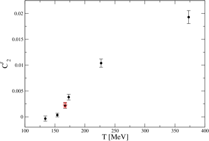
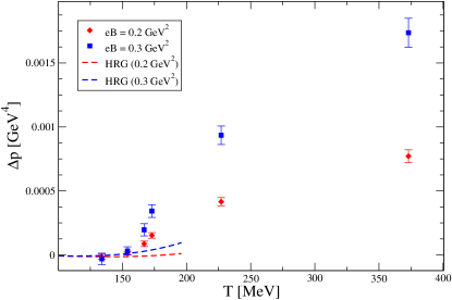
Figure 1: (Left panel) The second order coefficient in the Taylor expansion of $p/T^{4}$ vs. the temperature. The red empty circle at $T=167$ MeV denotes a value calculated at a larger spatial volume in order to check for finite volume effects. (Right panel) The $O(B^{2})$ thermal contribution to the pressure of the quark-gluon plasma due to the presence of a magnetic field, for two values $eB=0.2$ and 0.3 GeV². The HRG results are from Ref. Endrodi:2013cs .

In the right panel of Fig. 1 we show the thermal contribution to the pressure due to the presence of an external magnetic field to second order in the field i.e., without the vacuum pressure: $\Delta p=C^{r}_{2}(eB)^{2}$. We show $\Delta p$ for two values: $eB=0.2$ and 0.3 GeV². We compare it with predictions of the HRG model Endrodi:2013cs for the above fields (also with the vacuum pressure subtracted). Up to about 154 MeV the HRG and our result are roughly compatible (within large errors), and further studies should refine this statement. Of course, the HRG values contain terms of all possible orders, unlike our second-order-only result. At higher temperatures, the HRG and our results deviate, which is not surprising.

In light of our findings, it seems that the thermal correction of the pressure due to the presence of a magnetic field is small (within a few percent) for fields of $O(10^{15}{\rm T})$ [or equivalently $O(10^{-1}\rm GeV^{2})$], which are relevant for heavy-ion collision experiments. On the other hand, if in the early Universe fields reached $O(10^{16}{\rm T})$ [or $O(1\,\rm GeV^{2})$], this correction in the studied temperature range becomes large: roughly $20\%-100\%$ (with the larger value corresponding to lower temperatures). Of course, the latter statement assumes that using only the second order coefficient is sufficient to estimate $\Delta p$ in the presence of such a large external magnetic field.

In conclusion, in this work we argue for the feasibility and convenience of the Taylor expansion method for calculating the equation of state of the quark-gluon plasma in the presence of an external magnetic field. This work should be expanded in the future to include larger statistics, study of the finite volume effects at different temperatures, and contributions of higher orders in the Taylor expansion of the pressure. Other quantities such as the trace anomaly, energy density, effects on the chiral condensate, etc., can also be studied in this way with suitably higher statistics. (Results for some of these quantities obtained with other methods can be found in Refs. Bali:2013esa ; Bonati:2013lca ; others .)

Acknowledgements

We thank Urs Heller and Gergely Endrödi for helpful discussions. Computations for this work were carried out with resources provided by the USQCD Collaboration, the University of Utah Center for High Performance Computing, and Indiana University. This work was supported in part by the U.S National Science Foundation under Grant No. PHY10-67881 and the U.S. Department of Energy under Grant No. DE-FC02-12ER-41879.

References

- (1) D. Grasso and H. R. Rubinstein, Phys. Rept. 348, 163 (2001) [astro-ph/0009061].
- (2) A. Broderick, M. Prakash and J. M. Lattimer, Astrophys. J. 537, 351 (2000). C. Y. Cardall, M. Prakash, and J. M. Lattimer, Astrophys. J. 554, 322 (2001); A. Rabhi and C. Providencia, J. Phys. G: Nucl. Part. Phys. 35, 125201 (2008); A. Rabhi, P. K. Panda and C. Providencia, Phys. Rev. C 84, 035803 (2011) [arXiv:1105.0254 [nucl-th]].
- (3) J. Rafelski and B. Muller, Phys. Rev. Lett. 36, 517 (1976); D. E. Kharzeev, L. D. McLerran, and H. J. Warringa, Nucl. Phys. A 803, 227 (2008) [arXiv:0711.0950 [hep-ph]]; L. Ou and B. -A. Li, Phys. Rev. C 84, 064605 (2011) [arXiv:1107.3192 [nucl-th]].
- (4) G. Endrödi, J. High Energy Phys. 1304, 023 (2013) [arXiv:1301.1307 [hep-ph]].
- (5) M. H. Al-Hashimi and U. -J. Wiese, Ann. Phys. (N.Y.) 324, 343 (2009) [arXiv:0807.0630 [quant-ph]].
- (6) H. R. Rubinstein, S. Solomon, and T. Wittlich, Nucl. Phys. B 457, 577 (1995) [hep-lat/9501001].
- (7) G. S. Bali, F. Bruckmann, G. Endrödi, F. Gruber, and A. Schaefer, J. High Energy Phys. 1304, 130 (2013) [arXiv:1303.1328 [hep-lat]].
- (8) E. Follana et al. (HPQCD Collaboration and UKQCD Collaboration), Phys. Rev. D 75 054502 (2007), [arXiv:hep-lat/0610092]; C. Bernard et al., Phys. Rev. D 77, 014503 (2008) [arXiv:0710.1330 [hep-lat]]; C. DeTar et al., Phys. Rev. D 81, 114504 (2010) [arXiv:1003.5682 [hep-lat]].
- (9) C. Bonati, M. D’Elia, M. Mariti, F. Negro, and F. Sanfilippo, Phys. Rev. Lett. 111, 182001 (2013) [arXiv:1307.8063 [hep-lat]].
- (10) A. Bazavov et al. (HotQCD Collaboration), Phys. Rev. D 85, 054503 (2012) [arXiv:1111.1710 [hep-lat]].
- (11) M. A. Clark et al., Comput. Phys. Commun. 181, 1517 (2010) [arXiv:0911.3191 [hep-lat]]; R. Babich et al. [arXiv:1109.2935 [hep-lat]].
- (12) M. D’Elia, S. Mukherjee, and F. Sanfilippo, Phys. Rev. D 82, 051501 (2010) [arXiv:1005.5365 [hep-lat]]; M. D’Elia and F. Negro, Phys. Rev. D 83, 114028 (2011) [arXiv:1103.2080 [hep-lat]]; G. S. Bali, F. Bruckmann, G. Endrodi, Z. Fodor, S. D. Katz, and A. Schafer, Phys. Rev. D 86, 071502 (2012) [arXiv:1206.4205 [hep-lat]]; G. S. Bali et al., PoS Confinement X 197 (2012) [arXiv:1301.5826 [hep-lat]].